Error analysis for circle fitting algorithms

Abstract

We study the problem of fitting circles (or circular arcs) to data points observed with errors in both variables. A detailed error analysis for all popular circle fitting methods – geometric fit, Kåsa fit, Pratt fit, and Taubin fit – is presented. Our error analysis goes deeper than the traditional expansion to the leading order. We obtain higher order terms, which show exactly why and by how much circle fits differ from each other. Our analysis allows us to construct a new algebraic (non-iterative) circle fitting algorithm that outperforms all the existing methods, including the (previously regarded as unbeatable) geometric fit.

Keywords: least squares fit, curve fitting, circle fitting, algebraic fit, error analysis, variance, bias, functional model.

1 Introduction

Fitting circles and circular arcs to observed points is one of the basic tasks in pattern recognition and computer vision, nuclear physics, and other areas [5, 9, 11, 23, 24, 27, 30, 32]. Many algorithms have been developed that fit circles to data. Some minimize the geometric distances from the circle to the data points (we call them geometric fits). Others minimize various approximate (or ‘algebraic’) distances, they are called algebraic fits. We overview most popular algorithms in Sections 3–4.

Geometric fit is commonly regarded as the most accurate, but it can only be implemented by iterative schemes that are computationally intensive and subject to occasional divergence. Algebraic fits are faster but presumably less precise. At the same time the assessments on their accuracy are solely based on practical experience, no one has performed a detailed theoretical comparison of the accuracy of various circle fits. It was shown in [8] that all the circle fits have the same covariance matrix, to the leading order, in the small-noise limit. Thus the differences between various fits can only be revealed by a higher-order error analysis.

The purpose of this paper is to do just that. We employ higher-order error analysis (a similar analysis was used by Kanatani [22] in the context of more general quadratic models) and show exactly why and by how much the geometric circle fit outperforms the algebraic circle fits in accuracy; we also compare the precision of different algebraic fits. Section 5 presents our error analysis in a general form, which can be readily applied to other curve fitting problems.

Finally, our analysis allows us to develop a new algebraic fit whose accuracy exceeds that of the geometric fit. Its superiority is demonstrated by numerical experiments.

2 Statistical model

We adopt a standard functional model in which data points $(x_{1},y_{1}),\ldots,(x_{n},y_{n})$ are noisy observations of some true points $(\tilde{x}_{1},\tilde{y}_{1}),\ldots,(\tilde{x}_{n},\tilde{y}_{n})$, i.e.

(1) $$x_{i}=\tilde{x}_{i}+\delta_{i},\qquad y_{i}=\tilde{y}_{i}+\varepsilon_{i},\qquad i=1,\ldots,n,$$

where $(\delta_{i},\varepsilon_{i})$ represent isotropic Gaussian noise. Precisely, $\delta_{i}$’s and $\varepsilon_{i}$’s are i.i.d. normal random variables with mean zero and variance $\sigma^{2}$.

The true points $(\tilde{x}_{i},\tilde{y}_{i})$ are supposed to lie on a ‘true circle’, i.e. satisfy

(2) $$(\tilde{x}_{i}-\tilde{a})^{2}+(\tilde{y}_{i}-\tilde{b})^{2}=\tilde{R}^{2},\qquad i=1,\ldots,n,$$

where $(\tilde{a},\tilde{b},\tilde{R})$ denote the ‘true’ (unknown) parameters. Therefore

(3) $$\tilde{x}_{i}=\tilde{a}+\tilde{R}\cos\varphi_{i},\qquad\tilde{y}_{i}=\tilde{b}+\tilde{R}\sin\varphi_{i},$$

where $\varphi_{1},\ldots,\varphi_{n}$ specify the locations of the true points on the true circle. The angles $\varphi_{1},\ldots,\varphi_{n}$ are regarded as fixed unknowns and treated as additional parameters of the model (called incidental or latent parameters). For brevity we denote

(4) $$\tilde{u}_{i}=\cos\varphi_{i}=(\tilde{x}_{i}-\tilde{a})/\tilde{R},\qquad\tilde{v}_{i}=\sin\varphi_{i}=(\tilde{y}_{i}-\tilde{b})/\tilde{R}.$$

Note that $\tilde{u}_{i}^{2}+\tilde{v}_{i}^{2}=1$ for every $i$.

Remark. In our paper $\delta_{i}$ and $\varepsilon_{i}$ have common variance $\sigma^{2}$, i.e. our noise is homoscedastic. In many studies the noise is heteroscedastic [25, 35], i.e. the normal vector $(\delta_{i},\varepsilon_{i})$ has point-dependent covariance matrix $\sigma^{2}C_{i}$, where $C_{i}$ is known and depends on $i$, and $\sigma^{2}$ is an unknown factor. Our analysis can be extended to this case, too, but the resulting formulas will be somewhat more complex, so we leave it out.

3 Geometric circle fits

A standard approach to fitting circles to 2D data is based on orthogonal least squares, it is also called geometric fit, or orthogonal distance regression (ODR). It minimizes the function

(5) $$\mathcal{F}(a,b,R)=\sum d_{i}^{2},$$

where $d_{i}$ stands for the distance from $(x_{i},y_{i})$ to the circle, i.e.

(6) $$d_{i}=r_{i}-R,\qquad r_{i}=\sqrt{(x_{i}-a)^{2}+(y_{i}-b)^{2}},$$

where $(a,b)$ denotes the center, and $R$ the radius of the circle.

In the context of the functional model, the geometric fit returns the maximum likelihood estimates (MLE) of the circle parameters [6], i.e.

(7) $$(\hat{a}_{\rm MLE},\hat{b}_{\rm MLE},\hat{R}_{\rm MLE})=\,{\rm argmin}\,\mathcal{F}(a,b,R).$$

A major concern with the geometric fit is that the above minimization problem has no closed form solution. All practical algorithms of minimizing $\mathcal{F}$ are iterative; some implement a general Gauss-Newton [6, 15] or Levenberg-Marquardt [9] schemes, others use circle-specific methods proposed by Landau [24] and Späth [30]. The performance of iterative algorithms heavily depends on the choice of the initial guess. They often take dozens or hundreds of iterations to converge, and there is always a chance that they would be trapped in a local minimum of $\mathcal{F}$ or diverge entirely. These issues are explored in [9].

A peculiar feature of the maximum likelihood estimates $(\hat{a},\hat{b},\hat{R})$ of the circle parameters is that they have infinite moments [7], i.e.

(8) $${\mathbb{E}}(|\hat{a}|)={\mathbb{E}}(|\hat{b}|)={\mathbb{E}}(\hat{R})=\infty$$

for any set of true values $(\tilde{a},\tilde{b},\tilde{R})$; here ${\mathbb{E}}$ denotes the mean value. This happens because the distributions of these estimates have somewhat heavy tails, even though those tails barely affect the practical performance of the MLE (the same happens when one fits straight lines to data with errors in both variables [2, 3]).

To ensure the existence of moments one can adopt a different parameter scheme. An elegant scheme was proposed by Pratt [27] and others [13], which describes circles by an algebraic equation

(9) $$A(x^{2}+y^{2})+Bx+Cy+D=0$$

with an obvious constraint $A\neq 0$ (otherwise this equation describes a line) and a less obvious constraint $B^{2}+C^{2}-4AD>0$. The necessity of the latter can be seen if one rewrites equation (9) as

(10) $$\Bigl{(}x-\frac{B}{2A}\Bigr{)}^{2}+\Bigl{(}y-\frac{C}{2A}\Bigr{)}^{2}-\frac{B^{2}+C^{2}-4AD}{4A^{2}}=0.$$

It is clear now that (9) defines a circle if and only if $B^{2}+C^{2}-4AD>0$.

As the parameters $(A,B,C,D)$ only need to be determined up to a scalar multiple, it is natural to impose a constraint

(11) $$B^{2}+C^{2}-4AD=1,$$

because it automatically ensures $B^{2}+C^{2}-4AD>0$. The constraint (11) was first proposed by Pratt [27]. Under this constraint, the parameters $A,B,C,D$ are essentially bounded, see [9], and their maximum likelihood estimates can be shown to have finite moments.

The equation (9), under the constraint (11), conveniently describes all circles and lines (the latter are obtained when $A=0$); the inclusion of lines is necessary to ensure the existence of the least squares solution [9, 26, 37].

After one estimates the algebraic circle parameters $A,B,C,D$, they can be converted to the natural parameters via

(12) $$a=-\frac{B}{2A},\qquad b=-\frac{C}{2A},\qquad R^{2}=\frac{B^{2}+C^{2}-4AD}{4A^{2}}.$$

4 Algebraic circle fits

An alternative to the complicated geometric fit is made by fast non-iterative procedures called algebraic fits. We describe three most popular algebraic circle fits below.

Kåsa fit. One can find a circle by minimizing the function

$$\mathcal{F}_{\rm K} =\sum(r_{i}^{2}-R^{2})^{2}$$

(13) $$=\sum(x_{i}^{2}+y_{i}^{2}-2ax_{i}-2by_{i}+a^{2}+b^{2}-R^{2})^{2}.$$

In other words, one minimizes $\mathcal{F}_{\rm K}=\sum f_{i}^{2}$, where $f_{i}=r_{i}^{2}-R^{2}$ is the so called algebraic distance from the point $(x_{i},y_{i})$ to the circle. A change of parameters $B=-2a$, $C=-2b$, $D=a^{2}+b^{2}-R^{2}$ transforms (4) to a linear least squares problem minimizing

(14) $$\mathcal{F}_{\rm K}=\sum(z_{i}+Bx_{i}+Cy_{i}+D)^{2},$$

where we denote $z_{i}=x_{i}^{2}+y_{i}^{2}$ for brevity (we intentionally omit symbol $A$ here to make our formulas consistent with the subsequent ones). Now the problem reduces to a system of linear equations (normal equations) with respect to $B,C,D$ that can be easily solved, and then one recovers the natural circle parameters $a,b,R$ via (12).

This method was introduced in the 1970s by Delogne [11] and Kåsa [23], and then rediscovered and published independently by many authors, see references in [9]. It remains popular in practice. We call it Kåsa fit.

The Kåsa method is perhaps the fastest circle fit, but its accuracy suffers when one observes incomplete circular arcs (partially occluded circles); then the Kåsa fit is known to be heavily biased toward small circles [9]. The reason for the bias is that the algebraic distances $f_{i}$ provide a poor approximation to the geometric distances $d_{i}$; in fact,

(15) $$f_{i}=(r_{i}-R)(r_{i}+R)=d_{i}(2R+d_{i})\approx 2Rd_{i},$$

hence the Kåsa fit minimizes $\mathcal{F}_{\rm K}\approx 2R^{2}\sum d_{i}^{2}$, and it often favors smaller circles minimizing $R^{2}$ rather than the distances $d_{i}$.

Pratt fit. To improve the performance of the Kåsa method one can minimize another function, $\mathcal{F}=\frac{1}{4R^{2}}\mathcal{F}_{\rm K}$, which provides a better approximation to $\sum d_{i}^{2}$. This new function, expressed in terms of $A,B,C,D$ reads

(16) $$\mathcal{F}_{\rm P}=\sum\frac{[Az_{i}+Bx_{i}+Cy_{i}+D]^{2}}{B^{2}+C^{2}-4AD},$$

due to (12). Equivalently, one can minimize

(17) $$\mathcal{F}(A,B,C,D)=\sum[Az_{i}+Bx_{i}+Cy_{i}+D]^{2}$$

subject to the constraint (11). This method was proposed by Pratt [27].

Taubin fit. A slightly different method was proposed by Taubin [32] who minimizes the function

(18) $$\mathcal{F}_{\rm T}=\frac{\sum\bigl{[}(x_{i}-a)^{2}+(y_{i}-b)^{2}-R^{2}\bigr{]}^{2}}{4n^{-1}\sum\bigl{[}(x_{i}-a)^{2}+(y_{i}-b)^{2}\bigr{]}}.$$

Expressing it in terms of $A,B,C,D$ gives

(19) $$\mathcal{F}_{\rm T}=\sum\frac{[Az_{i}+Bx_{i}+Cy_{i}+D]^{2}}{n^{-1}\sum[4A^{2}z_{i}+4ABx_{i}+4ACy_{i}+B^{2}+C^{2}]}.$$

Equivalently, one can minimize (17) subject to a new constraint

(20) $$4A^{2}\bar{z}+4AB\bar{x}+4AC\bar{y}+B^{2}+C^{2}=1.$$

Here we use standard ‘sample means’ notation: $\bar{x}=\frac{1}{n}\sum x_{i}$, etc.

General remarks. Note that the minimization of (17) must use some constraint, to avoid a trivial solution $A=B=C=D=0$. Pratt and Taubin fits utilize constraints (11) and (20), respectively. Kåsa fit also minimizes (17), but subject to constraint $A=1$.

While the Pratt and Taubin estimates of the parameters $A,B,C,D$ have finite moments, the corresponding estimates of $a,b,R$ have infinite moments, just like the MLE (8). On the other hand, Kåsa’s estimates of $a,b,R$ have finite moments whenever $n\geq 4$; see [37].

All the above circle fits have an important property – they are independent of the choice of the coordinate system, i.e. their results are invariant under translations and rotations; see a proof in [14].

Practical experience shows that the Pratt and Taubin fits are more stable and accurate than the Kåsa fit, and they perform nearly equally well, see [9]. Taubin [32] intended to compare his fit to Pratt’s theoretically, but no such analysis was ever published. We make such a comparison below.

There are many other approaches to the circle fitting problem in the modern literature [4, 10, 35, 28, 29, 31, 33, 36, 38], but most of them are either quite slow or can be reduced to one of the algebraic fits [14, Chapter 8].

Matrix representation. We can represent the above three algebraic fits in matrix form. Let $\mathbf{A}=(A,B,C,D)$ denote the parameter vector,

(21) $$\mathbf{Z}\stackrel{{\scriptstyle\rm def}}{{=}}\left[\begin{array}[]{cccc}z_{1}&x_{1}&y_{1}&1\\ \vdots&\vdots&\vdots&\vdots\\ z_{n}&x_{n}&y_{n}&1\end{array}\right]$$

the ‘data matrix’ (recall that $z_{i}=x_{i}^{2}+y_{i}^{2})$ and

(22) $$\mathbf{M}\stackrel{{\scriptstyle\rm def}}{{=}}\frac{1}{n}\,\mathbf{Z}^{T}\mathbf{Z}=\left[\begin{array}[]{cccc}\overline{zz}&\overline{zx}&\overline{zy}&\bar{z}\\ \overline{zx}&\overline{xx}&\overline{xy}&\bar{x}\\ \overline{zy}&\overline{xy}&\overline{yy}&\bar{y}\\ \bar{z}&\bar{x}&\bar{y}&1\\ \end{array}\right]$$

the ‘matrix of moments’. All the algebraic circle fits minimize the same objective function ${\mathcal{F}}(\mathbf{A})=\mathbf{A}^{T}\mathbf{M}\mathbf{A}$, cf. (17), subject to a constraint $\mathbf{A}^{T}\mathbf{N}\mathbf{A}=1$, where the matrix $\mathbf{N}$ corresponds to the fit. The Pratt fit uses

(23) $$\mathbf{N}=\mathbf{P}\stackrel{{\scriptstyle\rm def}}{{=}}\left[\begin{array}[]{rrrr}0&0&0&-2\\ 0&1&0&0\\ 0&0&1&0\\ -2&0&0&0\end{array}\right],$$

the Taubin fit uses

(24) $$\mathbf{N}=\mathbf{T}\stackrel{{\scriptstyle\rm def}}{{=}}\left[\begin{array}[]{cccc}4\bar{z}&2\bar{x}&2\bar{y}&0\\ 2\bar{x}&1&0&0\\ 2\bar{y}&0&1&0\\ 0&0&0&0\end{array}\right],$$

and the Kåsa uses $\mathbf{N}=\mathbf{K}\stackrel{{\scriptstyle\rm def}}{{=}}\mathbf{e}_{1}\mathbf{e}_{1}^{T}$, where $\mathbf{e}_{1}=(1,0,0,0)^{T}$.

To solve the above constrained minimization problem one uses a Lagrange multiplier $\eta$ and reduces it to unconstrained minimization of the function

(25) $$\mathcal{G}(\mathbf{A},\eta)=\mathbf{A}^{T}\mathbf{M}\mathbf{A}-\eta(\mathbf{A}^{T}\mathbf{N}\mathbf{A}-1).$$

Differentiating with respect to $\mathbf{A}$ gives

(26) $$\mathbf{M}\mathbf{A}=\eta\mathbf{N}\mathbf{A},$$

thus $\mathbf{A}$ must be a generalized eigenvector for the matrix pair $(\mathbf{M},\mathbf{N})$. This fact is sufficient for the subsequent analysis, because it determines $\mathbf{A}$ up to a scalar multiple, and multiplying $\mathbf{A}$ by a scalar does not change the circle it represents, so we can set $\|\mathbf{A}\|=1$.

Remark. The generalized eigenvalue problem (26) may have several solutions. To choose the right one we note that for each solution $(\eta,\mathbf{A})$

$$\mathbf{A}^{T}\mathbf{M}\mathbf{A}=\eta\mathbf{A}^{T}\mathbf{N}\mathbf{A}=\eta,$$

thus for the purpose of minimizing $\mathbf{A}^{T}\mathbf{M}\mathbf{A}$ we should choose the solution of (26) with the smallest positive $\eta$.

5 Error Analysis: a general scheme

We employ an error analysis scheme based on a ‘small noise’ assumption. That is, we assume that the errors $\delta_{i}$ and $\varepsilon_{i}$ (Section 2) are small and treat their standard deviation $\sigma$ as a small parameter. The sample size $n$ is fixed, though it is not very small.

This approach goes back to Kadane [16] and was employed by Anderson [2] and other statisticians [3]. More recently it has been used by Kanatani [19, 22] in image processing applications, who argued that the ‘small noise’ model, where $\sigma\to 0$ while the sample size $n$ is kept fixed, is more appropriate than the traditional statistical ‘large sample’ approach, where $n\to\infty$ while $\sigma>0$ is kept fixed. We use a combination of these two models: our main assumption is $\sigma\to 0$, but $n$ is regarded as a slowly increasing parameter; more precisely we assume $n\ll\sigma^{-2}$.

Suppose one is fitting curves defined by an implicit equation

(27) $$P(x,y;{\boldsymbol{\Theta}})=0,$$

where ${\boldsymbol{\Theta}}=(\theta_{1},\ldots,\theta_{k})^{T}$ denotes a vector of unknown parameters to be estimated. Let $\tilde{{\boldsymbol{\Theta}}}=(\tilde{\theta}_{1},\ldots,\tilde{\theta}_{k})^{T}$ be the ’true’ parameter vector corresponding to the ‘true’ curve $P(x,y;\tilde{{\boldsymbol{\Theta}}})=0$. As in Section 2 let $(\tilde{x}_{i},\tilde{y}_{i})$, $i=1,\ldots,n$, denote true points, which lie on the true curve, and $(x_{i},y_{i})$ observed points satisfying (1). Let $\hat{{\boldsymbol{\Theta}}}(x_{1},y_{1},\ldots,x_{n},y_{n})$ be an estimator. We assume that $\hat{{\boldsymbol{\Theta}}}$ is a regular (at least four times differentiable) function of observations $(x_{i},y_{i})$. The existence of the derivatives of $\hat{{\boldsymbol{\Theta}}}$ is only required at the true points $(x_{i},y_{i})=(\tilde{x}_{i},\tilde{y}_{i})$, and it follows from the implicit function theorem under general assumptions provided $P(x,y;{\boldsymbol{\Theta}})$ in (27) is differentiable (in most cases $P$ is a polynomial in all its variables); we omit the proof.

For brevity we denote by $\mathbf{X}=(x_{1},y_{1},\ldots,x_{n},y_{n})^{T}$ the vector of all observations, so that $\mathbf{X}=\tilde{\mathbf{X}}+\mathbf{E}$, where $\tilde{\mathbf{X}}=(\tilde{x}_{1},\tilde{y}_{1},\ldots,\tilde{x}_{n},\tilde{y}_{n})^{T}$ is the vector of the true coordinates and $\mathbf{E}=(\delta_{1},\varepsilon_{1},\ldots,\delta_{n},\varepsilon_{n})^{T}$ is the ‘noise vector’; the components of $\mathbf{E}$ are i.i.d. normal random variables with mean zero and variance $\sigma^{2}$.

We use Taylor expansion to the second order terms. To keep our notation simple, we work with each scalar parameter $\theta_{m}$ of the vector ${\boldsymbol{\Theta}}$ separately:

(28) $$\hat{\theta}_{m}(\mathbf{X})=\hat{\theta}_{m}(\tilde{\mathbf{X}})+\mathbf{G}_{m}^{T}\mathbf{E}+\tfrac{1}{2}\,\mathbf{E}^{T}\mathbf{H}_{m}\mathbf{E}+\mathcal{O}_{P}(\sigma^{3}).$$

Here $\mathbf{G}_{m}=\nabla\hat{\theta}_{m}$ and $\mathbf{H}_{m}=\nabla^{2}\hat{\theta}_{m}$ denote the gradient (the vector of the first order partial derivatives) and the Hessian matrix of the second order partial derivatives of $\hat{\theta}_{m}$, respectively, taken at the true vector $\tilde{\mathbf{X}}$. The remainder term $\mathcal{O}_{P}(\sigma^{3})$ in (28) is a random variable $\mathcal{R}$ such that $\sigma^{-3}\mathcal{R}$ is bounded in probability.

Expansion (28) shows that $\hat{{\boldsymbol{\Theta}}}(\mathbf{X})\to\hat{{\boldsymbol{\Theta}}}(\tilde{\mathbf{X}})$ in probability, as $\sigma\to 0$. It is convenient to assume that

(29) $$\hat{{\boldsymbol{\Theta}}}(\tilde{\mathbf{X}})=\tilde{\boldsymbol{\Theta}}.$$

Precisely (29) means that whenever $\sigma=0$, i.e. when the true points are observed without noise, then the estimator returns the true parameter vector, i.e. finds the true curve. Geometrically, it means that if there is a model curve that interpolates the data points, then the algorithm finds it.

With some degree of informality, one can assert that whenever (29) holds, the estimate $\hat{{\boldsymbol{\Theta}}}$ is consistent in the limit $\sigma\to 0$. This is regarded as a minimal requirement for any sensible fitting algorithm. For example, if the observed points lie on one circle, then every circle fitting algorithm finds that circle uniquely. Kanatani [20] remarks that algorithms which fail to follow this property “are not worth considering”.

Under the assumption (29) we rewrite (28) as

(30) $$\Delta\hat{\theta}_{m}(\mathbf{X})=\mathbf{G}_{m}^{T}\mathbf{E}+\tfrac{1}{2}\,\mathbf{E}^{T}\mathbf{H}_{m}\mathbf{E}+\mathcal{O}_{P}(\sigma^{3}),$$

where $\Delta\hat{\theta}_{m}(\mathbf{X})=\hat{\theta}_{m}(\mathbf{X})-\tilde{\theta}_{m}$ is the statistical error of the parameter estimate.

The accuracy of an estimator $\hat{\theta}$ in statistics is characterized by its Mean Squared Error (MSE)

(31) $${\mathbb{E}}\bigl{[}(\hat{\theta}-\tilde{\theta})^{2}\bigr{]}={\sf Var}(\hat{\theta})+\bigr{[}{\rm bias}(\hat{\theta})\bigr{]}^{2},$$

where ${\rm bias}(\hat{\theta})={\mathbb{E}}(\hat{\theta})-\tilde{\theta}$. But it often happens that exact (or even approximate) values of ${\mathbb{E}}(\hat{\theta})$ and ${\sf Var}(\hat{\theta})$ are unavailable because the probability distribution of $\hat{\theta}$ is overly complicated, which is common in curve fitting problems, even if one fits straight lines to data points; see [2, 3]. There are also cases where the estimates have theoretically infinite moments because of somewhat heavy tails, which on the other hand barely affect their practical performance. Thus their accuracy should not be characterized by the theoretical moments which happen to be affected by heavy tails; see also [2]. In all such cases one usually constructs a good approximate probability distribution for $\hat{\theta}$ and judges the quality of $\hat{\theta}$ by the moments of that distribution.

It is standard [1, 2, 3, 12, 34] to construct a normal approximation to $\hat{\theta}$ and treat its variance as an ‘approximative’ MSE of $\hat{\theta}$. The normal approximation is usually based on the leading term in the Taylor expansion, like $\mathbf{G}_{m}^{T}\mathbf{E}$ in (30). For circle fitting algorithms, the resulting variance (see below) will be the same for all known methods, so we will go one step further and use the second order term. This gives us a better approximative distribution and allows us to compare circle fitting methods. In our formulas, ${\mathbb{E}}(\hat{\theta}_{m})$ and ${\sf Var}(\hat{\theta}_{m})$ denote the mean and variance of the resulting approximative distribution.

The first term in (30) is a linear combination of i.i.d. normal random variables that have zero mean, hence it is itself a normal random variable with zero mean. The second term is a quadratic form of i.i.d. normal variables. Since $\mathbf{H}_{m}$ is a symmetric matrix, we have $\mathbf{H}_{m}=\mathbf{Q}_{m}^{T}\mathbf{D}_{m}\mathbf{Q}_{m}$, where $\mathbf{Q}_{m}$ is an orthogonal matrix and $\mathbf{D}_{m}=\,{\rm diag}\{d_{1},\ldots,d_{2n}\}$ is a diagonal matrix. The vector $\mathbf{E}_{m}=\mathbf{Q}_{m}\mathbf{E}$ has the same distribution as $\mathbf{E}$ does, i.e. its components are i.i.d. normal random variables with mean zero and variance $\sigma^{2}$. Thus

(32) $$\mathbf{E}^{T}\mathbf{H}_{m}\mathbf{E}=\mathbf{E}_{m}^{T}\mathbf{D}_{m}\mathbf{E}_{m}=\sigma^{2}\sum d_{i}Z_{i}^{2},$$

where the $Z_{i}$’s are i.i.d. standard normal random variables, and the mean value of (32) is

(33) $${\mathbb{E}}\bigl{(}\mathbf{E}^{T}\mathbf{H}_{m}\mathbf{E}\bigr{)}=\sigma^{2}\,{\rm tr}\,\mathbf{D}_{m}=\sigma^{2}\,{\rm tr}\,\mathbf{H}_{m}.$$

Therefore, taking the mean value in (30) gives

(34) $${\rm bias}(\hat{\theta}_{m})={\mathbb{E}}(\Delta\hat{\theta}_{m})=\tfrac{1}{2}\,\sigma^{2}\,{\rm tr}\,\mathbf{H}_{m}+\mathcal{O}(\sigma^{4}).$$

Note that the expectations of all third order terms vanish, because the components of $\mathbf{E}$ are independent and their first and third moments are zero; thus the remainder term is of order $\sigma^{4}$.

Squaring (30) and again using (32) give the mean squared error (MSE)

(35) $${\mathbb{E}}\bigl{(}[\Delta\hat{\theta}_{m}]^{2}\bigr{)}=\sigma^{2}\mathbf{G}_{m}^{T}\mathbf{G}_{m}+\tfrac{1}{4}\,\sigma^{4}\bigl{(}[{\rm tr}\,\mathbf{H}_{m}]^{2}+2\|\mathbf{H}_{m}\|_{F}^{2}\bigr{)}+\mathcal{R},$$

where $\|\mathbf{H}_{m}\|_{F}^{2}=\,{\rm tr}\,\mathbf{H}_{m}^{2}$ is the Frobenius norm (note that $\|\mathbf{H}_{m}\|_{F}^{2}=\|\mathbf{D}_{m}\|_{F}^{2}=\,{\rm tr}\,\mathbf{D}_{m}^{2}$). The remainder $\mathcal{R}$ includes terms of order $\sigma^{6}$, as well as some terms of order $\sigma^{4}$ that contain third order partial derivatives, such as $\partial^{3}\hat{\theta}_{m}/\partial x_{i}^{3}$ and $\partial^{3}\hat{\theta}_{m}/\partial x_{i}^{2}\partial x_{j}$. A similar expression can be derived for ${\mathbb{E}}\bigl{(}\Delta\hat{\theta}_{m}\Delta\hat{\theta}_{m^{\prime}}\bigr{)}$ for $m\neq m^{\prime}$, we omit it and only give the final formula below.

Classification of higher order terms. In the MSE expansion (35), the leading term $\sigma^{2}\mathbf{G}_{m}^{T}\mathbf{G}_{m}$ is the most significant. The terms of order $\sigma^{4}$ are often given by long complicated formulas. Even the expression for the bias (34) may contain several terms of order $\sigma^{2}$, as we will see below. Fortunately, it is possible to sort them out keeping only the most significant ones, see next.

Kanatani [22] recently derived formulas for the bias of certain ellipse fitting algorithms. First he found all the terms of order $\sigma^{2}$, but in the end he noticed that some terms were of order $\sigma^{2}$ (independent of $n$), while the others of order $\sigma^{2}/n$. The magnitude of the former was clearly larger than that of the latter, and when Kanatani made his conclusions he ignored the terms of order $\sigma^{2}/n$. Here we formalize Kanatani’s classification of higher order terms as follows:
– In the expression for the bias (34) we keep terms of order $\sigma^{2}$ (independent of $n$) and ignore terms of order $\sigma^{2}/n$.
– In the expression for the mean squared error (35) we keep terms of order $\sigma^{4}$ (independent of $n$) and ignore terms of order $\sigma^{4}/n$.

These rules agree with our assumption that not only $\sigma\to 0$, but also $n\to\infty$, although $n$ increases rather slowly ($n\ll 1/\sigma^{2}$). Such models were studied by Amemiya, Fuller and Wolter [1, 34] who made a more rigid assumption that $n\sim\sigma^{-a}$ for some $0<a<2$.

Now it turns out (we omit detailed proofs; see [14]) that the main term $\sigma^{2}\mathbf{G}_{m}^{T}\mathbf{G}_{m}$ in our expression for the MSE (35) is of order $\sigma^{2}/n$; so it will never be ignored. Of the fourth order terms, $\tfrac{1}{2}\,\sigma^{4}\|\mathbf{H}_{m}\|_{F}^{2}$ is of order $\sigma^{4}/n$, hence it will be discarded, and the same applies to all the terms involving third order partial derivatives mentioned above.

The bias $\sigma^{2}\,{\rm tr}\,\mathbf{H}_{m}$ in (34) is, generally, of order $\sigma^{2}$ (independent of $n$), thus its contribution to the mean squared error (35) is significant. However the full expression for the bias may contain terms of order $\sigma^{2}$ and of order $\sigma^{2}/n$, of which the latter will be ignored; see below.

Now the terms in (35) have the following orders of magnitude:

(36) $${\mathbb{E}}\bigl{(}[\Delta\hat{\theta}_{m}]^{2}\bigr{)}=\mathcal{O}(\sigma^{2}/n)+\mathcal{O}(\sigma^{4})+\mathcal{O}(\sigma^{4}/n)+\mathcal{O}(\sigma^{6}),$$

where each big-O simply indicates the order of the corresponding term in (35). It is interesting to roughly compare their values numerically. In typical computer vision applications, $\sigma$ does not exceed $0.05$; see [5]. The number of data points normally varies between 10-20 (on the low end) and a few hundred (on the high end). For simplicity, we can set $n\sim 1/\sigma$ for smaller samples and $n\sim 1/\sigma^{2}$ for larger samples. Then Table 1 presents the corresponding typical magnitudes of each of the four terms in (35).

	$\phantom{m}\sigma^{2}/n\phantom{m}$	$\phantom{m}\sigma^{4}\phantom{m}$	$\phantom{m}\sigma^{4}/n\phantom{m}$	$\phantom{m}\sigma^{6}\phantom{m}$
small samples ($n\sim 1/\sigma$)	$\sigma^{3}$	$\sigma^{4}$	$\sigma^{5}$	$\sigma^{6}$
large samples ($n\sim 1/\sigma^{2}$)	$\sigma^{4}$	$\sigma^{4}$	$\sigma^{6}$	$\sigma^{6}$

Table 1: The order of magnitude of the four terms in (35).

We see that for larger samples the fourth order term coming from the bias may be just as big as the leading second-order term, hence it would be unwise to ignore it. Earlier studies, see e.g. [5, 8, 17], usually focused on the leading, i.e. second-order, terms only, disregarding all the fourth-order terms, and this is where our analysis is different. We make one step further – we keep all the terms of order $\mathcal{O}(\sigma^{2}/n)$ and $\mathcal{O}(\sigma^{4})$. The less significant terms of order $\mathcal{O}(\sigma^{4}/n)$ and $\mathcal{O}(\sigma^{6})$ would be discarded.

Now combining all our results gives a matrix formula for the (total) mean squared error (MSE)

(37) $${\mathbb{E}}\Bigl{[}(\Delta\hat{{\boldsymbol{\Theta}}})(\Delta\hat{{\boldsymbol{\Theta}}})^{T}\Bigr{]}=\sigma^{2}\mathbf{G}\mathbf{G}^{T}+\sigma^{4}\mathbf{B}\mathbf{B}^{T}+\cdots,$$

where $\mathbf{G}$ is the $k\times 2n$ matrix of first order partial derivatives of $\hat{{\boldsymbol{\Theta}}}(\mathbf{X})$, its rows are $\mathbf{G}_{m}^{T}$, $1\leq m\leq k$, and $\mathbf{B}=\tfrac{1}{2}[\,{\rm tr}\,\mathbf{H}_{1},\ldots\,{\rm tr}\,\mathbf{H}_{k}]^{T}$ is the $k$-vector that represents the leading term of the bias of $\hat{{\boldsymbol{\Theta}}}$, cf. (34). The trailing dots in (37) stand for all insignificant terms (those of order $\sigma^{4}/n$ and $\sigma^{6}$).

We call the first (main) term $\sigma^{2}\mathbf{G}\mathbf{G}^{T}$ in (37) the variance term, as it characterizes the variance (more precisely, the covariance matrix) of the estimator $\hat{{\boldsymbol{\Theta}}}$, to the leading order. For brevity we denote $\mathbf{V}=\mathbf{G}\mathbf{G}^{T}$. The second term $\sigma^{4}\mathbf{B}\mathbf{B}^{T}$ is the ‘tensor square’ of the bias $\sigma^{2}\mathbf{B}$ of the estimator, again to the leading order. When we deal with particular estimators in the next sections, we will see that the actual expression for the bias is a sum of terms of two types: some of them are of order $\mathcal{O}(\sigma^{2})$ and some others are of order $\mathcal{O}(\sigma^{2}/n)$, i.e.

(38) $${\mathbb{E}}(\Delta\hat{{\boldsymbol{\Theta}}})=\sigma^{2}\mathbf{B}+\mathcal{O}(\sigma^{4})=\sigma^{2}\mathbf{B}_{1}+\sigma^{2}\mathbf{B}_{2}+\mathcal{O}(\sigma^{4}),$$

where $\mathbf{B}_{1}=\mathcal{O}(1)$ and $\mathbf{B}_{2}=\mathcal{O}(1/n)$. We call $\sigma^{2}\mathbf{B}_{1}$ the essential bias of the estimator $\hat{{\boldsymbol{\Theta}}}$. This is its bias to the leading order, $\sigma^{2}$. The other terms, i.e. $\sigma^{2}\mathbf{B}_{2}$, and $\mathcal{O}(\sigma^{4})$, constitute non-essential bias; they can be discarded. Now (37) can be written as

(39) $${\mathbb{E}}\Bigl{[}(\Delta\hat{{\boldsymbol{\Theta}}})(\Delta\hat{{\boldsymbol{\Theta}}})^{T}\Bigr{]}=\sigma^{2}\mathbf{V}+\sigma^{4}\mathbf{B}_{1}\mathbf{B}_{1}^{T}+\cdots,$$

where we only keep significant terms of order $\sigma^{2}/n$ and $\sigma^{4}$ and drop the rest.

KCR lower bound. The matrix $\mathbf{V}$ representing the leading terms of the variance has a natural lower bound (an analogue of the Cramer-Rao bound): for every curve family (27) there is a symmetric positive semi-definite matrix $\mathbf{V}_{\min}$ such that for every estimator satisfying (29)

(40) $$\mathbf{V}\geq\mathbf{V}_{\min}=\biggl{(}\sum\frac{P_{{\boldsymbol{\Theta}}i}\,P_{{\boldsymbol{\Theta}}i}^{T}}{\|P_{\mathbf{x}i}\|^{2}}\biggr{)}^{-1},$$

in the sense that $\mathbf{V}-\mathbf{V}_{\min}$ is a positive semi-definite matrix. Here

(41) $$P_{{\boldsymbol{\Theta}}i}=\Bigl{(}\partial P(\tilde{\mathbf{x}}_{i};\tilde{{\boldsymbol{\Theta}}})/\partial\theta_{1},\ldots,\partial P(\tilde{\mathbf{x}}_{i};\tilde{{\boldsymbol{\Theta}}})/\partial\theta_{k}\Bigr{)}^{T}$$

stands for the gradient of $P$ with respect to the model parameters $\theta_{1},\ldots,\theta_{k}$ and

(42) $$P_{\mathbf{x}i}=\Bigl{(}\partial P(\tilde{\mathbf{x}}_{i};\tilde{{\boldsymbol{\Theta}}})/\partial x,\partial P(\tilde{\mathbf{x}}_{i};\tilde{{\boldsymbol{\Theta}}})/\partial y\Bigr{)}^{T}$$

for the gradient with respect to the planar variables $x$ and $y$; both gradients are taken at the true point $\tilde{\mathbf{x}}_{i}=(\tilde{x}_{i},\tilde{y}_{i})$. For example in the case of fitting circles defined by $P=(x-a)^{2}+(y-b)^{2}-R^{2}$, we have

(43) $$P_{{\boldsymbol{\Theta}}i}=-2\bigl{(}(\tilde{x}_{i}-\tilde{a}),(\tilde{y}_{i}-\tilde{b}),\tilde{R}\bigr{)}^{T},\qquad P_{\mathbf{x}i}=2\bigl{(}(\tilde{x}_{i}-\tilde{a}),(\tilde{y}_{i}-\tilde{b})\bigr{)}^{T}.$$

Therefore,

(44) $$\mathbf{V}_{\min}=(\mathbf{W}^{T}\mathbf{W})^{-1},$$

where

(45) $$\mathbf{W}\stackrel{{\scriptstyle\rm def}}{{=}}\left[\begin{array}[]{ccc}\tilde{u}_{1}&\tilde{v}_{1}&1\\ \vdots&\vdots&\vdots\\ \tilde{u}_{n}&\tilde{v}_{n}&1\\ \end{array}\right]$$

and $\tilde{u}_{i},\tilde{v}_{i}$ are given by (4).

The general inequality (40) was proved by Kanatani [17, 18] for unbiased estimators $\hat{{\boldsymbol{\Theta}}}$ and then extended by Chernov and Lesort [8] to all estimators satisfying (29). The geometric fit (which minimizes orthogonal distances) always satisfies (29) and attains the lower bound $\mathbf{V}_{\min}$; this was proved by Fuller (Theorem 3.2.1 in [12]) and independently by Chernov and Lesort [8], who named the inequality (40) Kanatani-Cramer-Rao (KCR) lower bound. See also survey [25] for the more general case of heteroscedastic noise.

Assessing the quality of estimators. Our analysis dictates the following strategy of assessing the quality of an estimator $\hat{{\boldsymbol{\Theta}}}$: first of all, its accuracy is characterized by the matrix $\mathbf{V}$, which must be compared to the KCR lower bound $\mathbf{V}_{\min}$. We will see that for all the circle fitting algorithms the matrix $\mathbf{V}$ actually achieves its lower bound $\mathbf{V}_{\min}$, i.e. we have $\mathbf{V}=\mathbf{V}_{\min}$, hence these algorithms are optimal to the leading order.

Next, once the factor $\mathbf{V}$ is already at its natural minimum, the accuracy of an estimator should be characterized by the vector $\mathbf{B}_{1}$ representing the essential bias – better estimates should have smaller essential biases. It appears that there is no natural minimum for $\|\mathbf{B}_{1}\|$, in fact there exist estimators which have a minimum variance $\mathbf{V}=\mathbf{V}_{\min}$ and a zero essential bias, i.e. $\mathbf{B}_{1}=\mathbf{0}$. We will construct such an estimator in Section 7.

6 Error analysis of geometric circle fit

Here we apply the general method of the previous section to the geometric circle fit, i.e. to the estimator $\hat{{\boldsymbol{\Theta}}}=(\hat{a},\hat{b},\hat{R})$ of the circle parameters minimizing the sum $\sum d_{i}^{2}$ of orthogonal (geometric) distances from the data points to the fitted circle.

Variance of the geometric circle fit. We start with the main part of our error analysis – the variance term represented by $\sigma^{2}\mathbf{V}$ in (39). The distances $d_{i}=r_{i}-R$ can be expanded as

$$d_{i} =\sqrt{\bigl{[}(\tilde{x}_{i}+\delta_{i})-(\tilde{a}+\Delta a)]^{2}+\bigl{[}(\tilde{y}_{i}+\varepsilon_{i})-(\tilde{b}+\Delta b)]^{2}}-\tilde{R}-\Delta R$$

$$=\sqrt{\tilde{R}^{2}+2\tilde{R}\tilde{u}_{i}(\delta_{i}-\Delta a)+2\tilde{R}\tilde{v}_{i}(\varepsilon_{i}-\Delta b)+\mathcal{O}_{P}(\sigma^{2})}-\tilde{R}-\Delta R$$

(46) $$=\tilde{u}_{i}(\delta_{i}-\Delta a)+\tilde{v}_{i}(\varepsilon_{i}-\Delta b)-\Delta R+\mathcal{O}_{P}(\sigma^{2}),$$

see (4). Minimizing $\sum d_{i}^{2}$ to the first order is equivalent to minimizing

(47) $$\sum(\tilde{u}_{i}\,\Delta a+\tilde{v}_{i}\,\Delta b+\Delta R-\tilde{u}_{i}\delta_{i}-\tilde{v}_{i}\varepsilon_{i})^{2}.$$

This is a classical least squares problem that can also be written as

(48) $$\mathbf{W}\,\Delta{\boldsymbol{\Theta}}\approx\tilde{\mathbf{U}}{\boldsymbol{\delta}}+\tilde{\mathbf{V}}{\boldsymbol{\varepsilon}},$$

where $\mathbf{W}$ is given by (45), ${\boldsymbol{\Theta}}=(a,b,R)^{T}$, as well as ${\boldsymbol{\delta}}=(\delta_{1},\ldots,\delta_{n})^{T}$ and ${\boldsymbol{\varepsilon}}=(\varepsilon_{1},\ldots,\varepsilon_{n})^{T}$, while $\tilde{\mathbf{U}}=\,{\rm diag}(\tilde{u}_{1},\ldots,\tilde{u}_{n})$ and $\tilde{\mathbf{V}}=\,{\rm diag}(\tilde{v}_{1},\ldots,\tilde{v}_{n})$. The solution of the least squares problem (48) is

(49) $$\Delta\hat{{\boldsymbol{\Theta}}}=(\mathbf{W}^{T}\mathbf{W})^{-1}\mathbf{W}^{T}(\tilde{\mathbf{U}}{\boldsymbol{\delta}}+\tilde{\mathbf{V}}{\boldsymbol{\varepsilon}}),$$

of course this does not include the $\mathcal{O}_{P}(\sigma^{2})$ terms. Thus the variance of our estimator, to the leading order, is

(50) $${\mathbb{E}}\bigl{[}(\Delta\hat{{\boldsymbol{\Theta}}})(\Delta\hat{{\boldsymbol{\Theta}}})^{T}\bigr{]}=(\mathbf{W}^{T}\mathbf{W})^{-1}\mathbf{W}^{T}{\mathbb{E}}\bigl{[}(\tilde{\mathbf{U}}{\boldsymbol{\delta}}+\tilde{\mathbf{V}}{\boldsymbol{\varepsilon}})({\boldsymbol{\delta}}^{T}\tilde{\mathbf{U}}+{\boldsymbol{\varepsilon}}^{T}\tilde{\mathbf{V}})\bigr{]}\mathbf{W}(\mathbf{W}^{T}\mathbf{W})^{-1}.$$

Now observe that ${\mathbb{E}}({\boldsymbol{\delta}}{\boldsymbol{\varepsilon}}^{T})={\mathbb{E}}({\boldsymbol{\varepsilon}}{\boldsymbol{\delta}}^{T})=\mathbf{0}$, as well as ${\mathbb{E}}({\boldsymbol{\delta}}{\boldsymbol{\delta}}^{T})={\mathbb{E}}({\boldsymbol{\varepsilon}}{\boldsymbol{\varepsilon}}^{T})=\sigma^{2}\mathbf{I}$, and we have $\tilde{\mathbf{U}}^{2}+\tilde{\mathbf{V}}^{2}=\mathbf{I}$. Thus to the leading order

(51) $${\mathbb{E}}\bigl{[}(\Delta\hat{{\boldsymbol{\Theta}}})(\Delta\hat{{\boldsymbol{\Theta}}})^{T}\bigr{]}=\sigma^{2}(\mathbf{W}^{T}\mathbf{W})^{-1}\mathbf{W}^{T}\mathbf{W}(\mathbf{W}^{T}\mathbf{W})^{-1}=\sigma^{2}(\mathbf{W}^{T}\mathbf{W})^{-1},$$

where the higher order (of $\sigma^{4}$) terms are not included. Comparing this to (44) confirms that the geometric fit attains the minimal possible covariance matrix $\mathbf{V}$.

Bias of the geometric circle fit. Now we do a second-order error analysis, which has not been previously done in the literature. According to a general formula (28), we put

(52) $$\begin{split}a&=\tilde{a}+\Delta_{1}a+\Delta_{2}a+\mathcal{O}_{P}(\sigma^{3}),\\ b&=\tilde{b}+\Delta_{1}b+\Delta_{2}b+\mathcal{O}_{P}(\sigma^{3}),\\ R&=\tilde{R}+\Delta_{1}R+\Delta_{2}R+\mathcal{O}_{P}(\sigma^{3}).\end{split}$$

Here $\Delta_{1}a$, $\Delta_{1}b$, $\Delta_{1}R$ are linear combinations of $\varepsilon_{i}$’s and $\delta_{i}$’s, which were found above, in (49), and $\Delta_{2}a$, $\Delta_{2}b$, $\Delta_{2}R$ are quadratic forms of $\varepsilon_{i}$’s and $\delta_{i}$’s to be determined next.

Expanding the distances $d_{i}$ to the second order terms gives

$$d_{i} =\tilde{u}_{i}(\delta_{i}-\Delta_{1}a)+\tilde{v}_{i}(\varepsilon_{i}-\Delta_{1}b)-\Delta_{1}R$$

$$\quad-\tilde{u}_{i}\,\Delta_{2}a-\tilde{v}_{i}\,\Delta_{2}b-\Delta_{2}R+\tfrac{\tilde{v}_{i}^{2}}{2\tilde{R}}(\delta_{i}-\Delta_{1}a)^{2}+\tfrac{\tilde{u}_{i}^{2}}{2\tilde{R}}(\varepsilon_{i}-\Delta_{1}b)^{2}$$

(53) $$\quad-\tfrac{\tilde{u}_{i}\tilde{v}_{i}}{\tilde{R}}(\delta_{i}-\Delta_{1}a)(\varepsilon_{i}-\Delta_{1}b).$$

Since we already found $\Delta_{1}a$, $\Delta_{1}b$, $\Delta_{1}R$, the only unknowns are $\Delta_{2}a$, $\Delta_{2}b$, $\Delta_{2}R$. Minimizing $\sum d_{i}^{2}$ is now equivalent to minimizing

(54) $$\sum(\tilde{u}_{i}\,\Delta_{2}a+\tilde{v}_{i}\,\Delta_{2}b+\Delta_{2}R-f_{i})^{2},$$

where

(55) $$f_{i} = \tilde{u}_{i}(\delta_{i}-\Delta_{1}a)+\tilde{v}_{i}(\varepsilon_{i}-\Delta_{1}b)-\Delta_{1}R$$

$$+ \tfrac{\tilde{v}_{i}^{2}}{2R}(\delta_{i}-\Delta_{1}a)^{2}+\tfrac{\tilde{u}_{i}^{2}}{2R}(\varepsilon_{i}-\Delta_{1}b)^{2}-\tfrac{\tilde{u}_{i}\tilde{v}_{i}}{R}(\delta_{i}-\Delta_{1}a)(\varepsilon_{i}-\Delta_{1}b).$$

This is another least squares problem, and its solution is

(56) $$\Delta_{2}\hat{{\boldsymbol{\Theta}}}=(\mathbf{W}^{T}\mathbf{W})^{-1}\mathbf{W}^{T}\mathbf{F},$$

where $\mathbf{F}=(f_{1},\ldots,f_{n})^{T}$; of course this is a quadratic approximation which does not include $\mathcal{O}_{P}(\sigma^{3})$ terms. In fact, the contribution from the first three (linear) terms in (55) vanishes, quite predictably; thus only the last two (quadratic) terms matter.

Taking the mean value gives, to the leading order,

(57) $${\mathbb{E}}(\Delta\hat{{\boldsymbol{\Theta}}})={\mathbb{E}}(\Delta_{2}\hat{{\boldsymbol{\Theta}}})=\frac{\sigma^{2}}{2R}\bigl{[}(\mathbf{W}^{T}\mathbf{W})^{-1}\mathbf{W}^{T}\mathbf{1}+(\mathbf{W}^{T}\mathbf{W})^{-1}\mathbf{W}^{T}\mathbf{S}\bigr{]},$$

where $\mathbf{1}=(1,1,\ldots,1)^{T}$ and $\mathbf{S}=(s_{1},\ldots,s_{n})^{T}$, here $s_{i}$ is a scalar

(58) $$s_{i}=[-\tilde{v}_{i},\tilde{u}_{i},0](\mathbf{W}^{T}\mathbf{W})^{-1}[-\tilde{v}_{i},\tilde{u}_{i},0]^{T}.$$

The second term in (57) is of order $\mathcal{O}(\sigma^{2}/n)$, thus the essential bias is given by the first term only, and it can be simplified. Since the last column of the matrix $\mathbf{W}^{T}\mathbf{W}$ coincides with the vector $\mathbf{W}^{T}\mathbf{1}$, we have $(\mathbf{W}^{T}\mathbf{W})^{-1}\mathbf{W}^{T}\mathbf{1}=[0,0,1]^{T}$, hence the essential bias of the geometric circle fit is

(59) $${\mathbb{E}}(\Delta\hat{{\boldsymbol{\Theta}}})\stackrel{{\scriptstyle\rm ess}}{{=}}\frac{\sigma^{2}}{2\tilde{R}}\,\bigl{[}0,0,1\bigr{]}^{T}.$$

Thus the estimates of the circle center, $\hat{a}$ and $\hat{b}$, have no essential bias, while the estimate of the radius has essential bias

(60) $${\mathbb{E}}(\Delta\hat{R})\stackrel{{\scriptstyle\rm ess}}{{=}}\frac{\sigma^{2}}{2\tilde{R}},$$

which is independent of the number and location of the true points. These facts are consistent with the results obtained by Berman [5] under the assumptions that $\sigma>0$ is fixed and $n\to\infty$.

7 Error analysis of algebraic circle fits

Here we analyze algebraic circle fits using their matrix representation.

Matrix perturbation method. For every random variable, matrix or vector, $\mathbf{L}$, we write

(61) $$\mathbf{L}=\tilde{\mathbf{L}}+\Delta_{1}\mathbf{L}+\Delta_{2}\mathbf{L}+\mathcal{O}_{P}(\sigma^{3}),$$

where $\tilde{\mathbf{L}}$ is its ‘true’, nonrandom, value (achieved when $\sigma=0$), $\Delta_{1}\mathbf{L}$ is a linear combination of $\delta_{i}$’s and $\varepsilon_{i}$’s, and $\Delta_{2}\mathbf{L}$ is a quadratic form of $\delta_{i}$’s and $\varepsilon_{i}$’s; all the higher order terms (cubic etc.) are represented by $\mathcal{O}_{P}(\sigma^{3})$. For brevity, we drop the $\mathcal{O}_{P}(\sigma^{3})$ terms in our formulas. Therefore $\mathbf{A}=\tilde{\mathbf{A}}+\Delta_{1}\mathbf{A}+\Delta_{2}\mathbf{A}$ and $\mathbf{M}=\tilde{\mathbf{M}}+\Delta_{1}\mathbf{M}+\Delta_{2}\mathbf{M}$, and (22) implies

(62) $$\Delta_{1}\mathbf{M} =n^{-1}(\tilde{\mathbf{Z}}^{T}\Delta_{1}\mathbf{Z}+\Delta_{1}\mathbf{Z}^{T}\tilde{\mathbf{Z}}),$$

(63) $$\Delta_{2}\mathbf{M} =n^{-1}(\Delta_{1}\mathbf{Z}^{T}\,\Delta_{1}\mathbf{Z}+\tilde{\mathbf{Z}}^{T}\,\Delta_{2}\mathbf{Z}+\Delta_{2}\mathbf{Z}^{T}\,\tilde{\mathbf{Z}}).$$

Since the true points lie on the true circle, $\tilde{\mathbf{Z}}\tilde{\mathbf{A}}=\mathbf{0}$, as well as $\tilde{\mathbf{M}}\tilde{\mathbf{A}}=\mathbf{0}$ (hence $\tilde{\mathbf{M}}$ is a singular matrix). Therefore

(64) $$\tilde{\mathbf{A}}^{T}\,\Delta_{1}\mathbf{M}\,\tilde{\mathbf{A}}=n^{-1}\tilde{\mathbf{A}}^{T}\bigl{(}\tilde{\mathbf{Z}}^{T}\,\Delta_{1}\mathbf{Z}+\Delta_{1}\mathbf{Z}^{T}\,\tilde{\mathbf{Z}}\bigr{)}\tilde{\mathbf{A}}=0,$$

hence $\mathbf{A}^{T}\mathbf{M}\mathbf{A}=\mathcal{O}_{P}(\sigma^{2})$, and premultiplying (26) by $\mathbf{A}^{T}$ yields $\eta=\mathcal{O}_{P}(\sigma^{2})$. Next, substituting the expansions of $\mathbf{M}$, $\mathbf{A}$, and $\mathbf{N}$ into (26) gives

(65) $$(\tilde{\mathbf{M}}+\Delta_{1}\mathbf{M}+\Delta_{2}\mathbf{M})(\tilde{\mathbf{A}}+\Delta_{1}\mathbf{A}+\Delta_{2}\mathbf{A})=\eta\tilde{\mathbf{N}}\tilde{\mathbf{A}}$$

(recall that $\mathbf{N}$ is data-dependent for the Taubin method, but only its ‘true’ value $\tilde{\mathbf{N}}$ matters, as $\eta=\mathcal{O}_{P}(\sigma^{2})$, hence the use of the observed values only adds higher order terms). Now using $\tilde{\mathbf{M}}\tilde{\mathbf{A}}=\mathbf{0}$ yields

(66) $$(\tilde{\mathbf{M}}\,\Delta_{1}\mathbf{A}+\Delta_{1}\mathbf{M}\,\tilde{\mathbf{A}})+(\tilde{\mathbf{M}}\,\Delta_{2}\mathbf{A}+\Delta_{1}\mathbf{M}\,\Delta_{1}\mathbf{A}+\Delta_{2}\mathbf{M}\,\tilde{\mathbf{A}})=\eta\tilde{\mathbf{N}}\tilde{\mathbf{A}}$$

The left hand side of (66) consists of a linear part $(\tilde{\mathbf{M}}\,\Delta_{1}\mathbf{A}+\Delta_{1}\mathbf{M}\,\tilde{\mathbf{A}})$ and a quadratic part $(\tilde{\mathbf{M}}\,\Delta_{2}\mathbf{A}+\Delta_{1}\mathbf{M}\,\Delta_{1}\mathbf{A}+\Delta_{2}\mathbf{M}\,\tilde{\mathbf{A}})$. Separating them gives

(67) $$\tilde{\mathbf{M}}\,\Delta_{1}\mathbf{A}+n^{-1}\tilde{\mathbf{Z}}^{T}\,\Delta_{1}\mathbf{Z}\,\tilde{\mathbf{A}}=\mathbf{0}$$

(where we used (62) and $\tilde{\mathbf{Z}}\tilde{\mathbf{A}}={\mathbf{0}}$) and

(68) $$\tilde{\mathbf{M}}\,\Delta_{2}\mathbf{A}+\Delta_{1}\mathbf{M}\,\Delta_{1}\mathbf{A}+\Delta_{2}\mathbf{M}\,\tilde{\mathbf{A}}=\eta\tilde{\mathbf{N}}\tilde{\mathbf{A}}.$$

Note that $\tilde{\mathbf{M}}$ is a singular matrix (because $\tilde{\mathbf{M}}\tilde{\mathbf{A}}=\mathbf{0}$), but whenever there are at least three distinct true points, they determine a unique true circle, thus the kernel of $\tilde{\mathbf{M}}$ is one-dimensional, and it coincides with span($\tilde{\mathbf{A}}$). Also, we set $\|\mathbf{A}\|=1$, hence $\Delta_{1}\mathbf{A}$ is orthogonal to $\tilde{\mathbf{A}}$, and we can write

(69) $$\Delta_{1}\mathbf{A}=-n^{-1}\tilde{\mathbf{M}}^{-}\tilde{\mathbf{Z}}^{T}\,\Delta_{1}\mathbf{Z}\,\tilde{\mathbf{A}},$$

where $\tilde{\mathbf{M}}^{-}$ denotes the Moore-Penrose pseudoinverse. Now one can easily check that ${\mathbb{E}}(\Delta_{1}\mathbf{M}\,\Delta_{1}\mathbf{A})=\mathcal{O}(\sigma^{2}/n)$ and ${\mathbb{E}}(\Delta_{1}\mathbf{A})=0$; these facts will be useful in the upcoming analysis.

Variance of algebraic circle fits. From (69) we conclude that

$${\mathbb{E}}\bigl{[}(\Delta_{1}\mathbf{A})(\Delta_{1}\mathbf{A})^{T}\bigr{]} =n^{-2}\tilde{\mathbf{M}}^{-}{\mathbb{E}}(\tilde{\mathbf{Z}}^{T}\,\Delta_{1}\mathbf{Z}\,\tilde{\mathbf{A}}\tilde{\mathbf{A}}^{T}\,\Delta_{1}\mathbf{Z}^{T}\,\tilde{\mathbf{Z}})\tilde{\mathbf{M}}^{-}$$

(70) $$=n^{-2}\tilde{\mathbf{M}}^{-}{\mathbb{E}}\Bigl{[}\bigl{(}\sum_{i}\tilde{\mathbf{Z}}_{i}\,\Delta_{1}\mathbf{Z}_{i}^{T}\bigr{)}\tilde{\mathbf{A}}\tilde{\mathbf{A}}^{T}\bigl{(}\sum_{j}\Delta_{1}\mathbf{Z}_{j}^{T}\,\tilde{\mathbf{Z}}_{j}^{T}\bigr{)}\Bigr{]}\tilde{\mathbf{M}}^{-},$$

where

(71) $$\tilde{\mathbf{Z}}_{i}\stackrel{{\scriptstyle\rm def}}{{=}}\left[\begin{array}[]{c}\tilde{z}_{i}\\ \tilde{x}_{i}\\ \tilde{y}_{i}\\ 1\end{array}\right]\qquad\text{and}\qquad\Delta_{1}\mathbf{Z}_{i}=\left[\begin{array}[]{c}2\tilde{x}_{i}\delta_{i}+2\tilde{y}_{i}\varepsilon_{i}\\ \delta_{i}\\ \varepsilon_{i}\\ 0\end{array}\right]$$

denote the columns of the matrices $\tilde{\mathbf{Z}}^{T}$ and $\Delta_{1}\mathbf{Z}^{T}$, respectively. Next,

(72) $${\mathbb{E}}\bigl{[}(\Delta_{1}\mathbf{Z}_{i})(\Delta_{1}\mathbf{Z}_{j})^{T}\bigr{]}=\left\{\begin{array}[]{cc}0&\qquad\text{whenever }\quad i\neq j\\ \sigma^{2}\tilde{\mathbf{T}}_{i}&\qquad\text{whenever }\quad i=j\end{array}\right.$$

where

(73) $$\tilde{\mathbf{T}}_{i}\stackrel{{\scriptstyle\rm def}}{{=}}\left[\begin{array}[]{cccc}4\tilde{z}_{i}&2\tilde{x}_{i}&2\tilde{y}_{i}&0\\ 2\tilde{x}_{i}&1&0&0\\ 2\tilde{y}_{i}&0&1&0\\ 0&0&0&0\end{array}\right].$$

Note $n^{-1}\sum\tilde{\mathbf{T}}_{i}=\tilde{\mathbf{T}}$ and $\tilde{\mathbf{A}}^{T}\tilde{\mathbf{T}}_{i}\tilde{\mathbf{A}}=\tilde{\mathbf{A}}^{T}\mathbf{P}\tilde{\mathbf{A}}=\tilde{B}^{2}+\tilde{C}^{2}-4\tilde{A}\tilde{D}$ for each $i$; recall (23) and (24). Hence

(74) $$\sum\tilde{\mathbf{Z}}_{i}\tilde{\mathbf{A}}^{T}\tilde{\mathbf{T}}_{i}\tilde{\mathbf{A}}\tilde{\mathbf{Z}}_{i}^{T}=\sum(\tilde{\mathbf{A}}^{T}\mathbf{P}\tilde{\mathbf{A}})\tilde{\mathbf{Z}}_{i}\tilde{\mathbf{Z}}_{i}^{T}=n(\tilde{\mathbf{A}}^{T}\mathbf{P}\tilde{\mathbf{A}})\tilde{\mathbf{M}}.$$

Combining the above formulas gives

$${\mathbb{E}}\bigl{[}(\Delta_{1}\mathbf{A})(\Delta_{1}\mathbf{A})^{T}\bigr{]} =n^{-2}\tilde{\mathbf{M}}^{-}\Bigl{[}\sum_{i,j}\tilde{\mathbf{Z}}_{i}\tilde{\mathbf{A}}^{T}{\mathbb{E}}\bigl{(}\Delta_{1}\mathbf{Z}_{i}^{T}\Delta_{1}\mathbf{Z}_{j}^{T}\bigr{)}\tilde{\mathbf{A}}\tilde{\mathbf{Z}}_{j}^{T}\Bigr{]}\tilde{\mathbf{M}}^{-}$$

$$=n^{-2}\sigma^{2}\tilde{\mathbf{M}}^{-}\Bigl{[}\sum\tilde{\mathbf{Z}}_{i}\tilde{\mathbf{A}}^{T}\tilde{\mathbf{T}}_{i}\tilde{\mathbf{A}}\tilde{\mathbf{Z}}_{i}^{T}\Bigr{]}\tilde{\mathbf{M}}^{-}$$

(75) $$=n^{-1}\sigma^{2}\tilde{\mathbf{M}}^{-}(\tilde{\mathbf{A}}^{T}\mathbf{P}\tilde{\mathbf{A}}).$$

Remarkably, the variance of algebraic fits does not depend on the constraint matrix $\mathbf{N}$, hence all algebraic fits have the same variance (to the leading order). In the next section we will derive the variance of algebraic fits in the natural circle parameters $(a,b,R)$ and see that it coincides with the variance of the geometric fit (51).

Bias of algebraic circle fits. Since ${\mathbb{E}}(\Delta_{1}\mathbf{A})=0$, it will be enough to find ${\mathbb{E}}(\Delta_{2}\mathbf{A})$. Premultiplying (68) by $\tilde{\mathbf{A}}^{T}$ yields

(76) $$\eta=\frac{\tilde{\mathbf{A}}^{T}\mathbf{M}\mathbf{A}}{\tilde{\mathbf{A}}^{T}\mathbf{N}\mathbf{A}}=\frac{\tilde{\mathbf{A}}^{T}\,\Delta_{2}\mathbf{M}\,\tilde{\mathbf{A}}+\tilde{\mathbf{A}}^{T}\,\Delta_{1}\mathbf{M}\,\Delta_{1}\mathbf{A}}{\tilde{\mathbf{A}}^{T}\tilde{\mathbf{N}}\tilde{\mathbf{A}}}+\mathcal{O}_{P}(\sigma^{2}/n).$$

Recall that ${\mathbb{E}}(\Delta_{1}\mathbf{M}\,\Delta_{1}\mathbf{A})=\mathcal{O}(\sigma^{2}/n)$, thus this term will not affect the essential bias and we drop it. Taking the mean value and using (69) gives

(77) $${\mathbb{E}}(\eta)=\frac{\tilde{\mathbf{A}}^{T}{\mathbb{E}}(\Delta_{2}\mathbf{M})\tilde{\mathbf{A}}}{\tilde{\mathbf{A}}^{T}\tilde{\mathbf{N}}\tilde{\mathbf{A}}}+\mathcal{O}(\sigma^{2}/n),$$

We substitute (63) into (76), use $\tilde{\mathbf{Z}}\tilde{\mathbf{A}}={\mathbf{0}}$, then observe that

(78) $${\mathbb{E}}(\Delta_{1}\mathbf{Z}^{T}\,\Delta_{1}\mathbf{Z}\tilde{\mathbf{A}})=\sigma^{2}\sum\tilde{\mathbf{T}}_{i}\tilde{\mathbf{A}}=2\tilde{A}\sigma^{2}\sum\tilde{\mathbf{Z}}_{i}+n\sigma^{2}\mathbf{P}\tilde{\mathbf{A}}$$

(here $\tilde{A}$ is the first component of the vector $\tilde{\mathbf{A}}$). Then, note that $\Delta_{2}\mathbf{Z}_{i}=(\delta_{i}^{2}+\varepsilon_{i}^{2},0,0,0)^{T}$, and so

(79) $${\mathbb{E}}(\tilde{\mathbf{Z}}^{T}\,\Delta_{2}\mathbf{Z})\tilde{\mathbf{A}}=2\tilde{A}\sigma^{2}\sum\tilde{\mathbf{Z}}_{i}.$$

Therefore the essential bias is given by

(80) $${\mathbb{E}}(\Delta_{2}\mathbf{A})\stackrel{{\scriptstyle\rm ess}}{{=}}-\sigma^{2}\tilde{\mathbf{M}}^{-}\Bigl{[}4\tilde{A}n^{-1}\sum\tilde{\mathbf{Z}}_{i}+\mathbf{P}\tilde{\mathbf{A}}-\frac{\tilde{\mathbf{A}}^{T}\mathbf{P}\tilde{\mathbf{A}}}{\tilde{\mathbf{A}}^{T}\tilde{\mathbf{N}}\tilde{\mathbf{A}}}\,\tilde{\mathbf{N}}\tilde{\mathbf{A}}\Bigr{]}.$$

A more detailed analysis (which we omit) gives the following expression containing all the $\mathcal{O}(\sigma^{2})$ and $\mathcal{O}(\sigma^{2}/n)$ terms:

$${\mathbb{E}}(\Delta_{2}\mathbf{A}) =-\sigma^{2}\tilde{\mathbf{M}}^{-}\Bigl{[}4\tilde{A}n^{-1}\sum\tilde{\mathbf{Z}}_{i}+(1-\tfrac{4}{n})\mathbf{P}\tilde{\mathbf{A}}-\frac{(1-\tfrac{3}{n})(\tilde{\mathbf{A}}^{T}\mathbf{P}\tilde{\mathbf{A}})}{\tilde{\mathbf{A}}^{T}\tilde{\mathbf{N}}\tilde{\mathbf{A}}}\,\tilde{\mathbf{N}}\tilde{\mathbf{A}}$$

(81) $$\quad-4\tilde{A}n^{-2}\sum(\tilde{\mathbf{Z}}_{i}^{T}\tilde{\mathbf{M}}^{-}\tilde{\mathbf{Z}}_{i})\tilde{\mathbf{Z}}_{i}\Bigr{]}+\mathcal{O}(\sigma^{4}).$$

This expression demonstrates that the terms of order $\sigma^{2}/n$ (the non-essential bias) only add a small correction, which is negligible when $n$ is large.

The expressions (80) and (7) can be simplified. Note that the vector $n^{-1}\sum\tilde{\mathbf{Z}}_{i}$ coincides with the last column of the matrix $\tilde{\mathbf{M}}$, hence

(82) $$-\sigma^{2}\tilde{\mathbf{M}}^{-}\Bigl{[}4\tilde{A}n^{-1}\sum\tilde{\mathbf{Z}}_{i}\Bigr{]}=-4\sigma^{2}\tilde{A}\,[0,0,0,1]^{T}.$$

In fact, this term will play the key role in the subsequent analysis.

8 Comparison of various circle fits

Bias of the Pratt and Taubin fits. We have seen that all the algebraic fits have the same main characteristic – the variance (75), to the leading order. We will see below that their variance coincides with that of the geometric circle fit. Thus the difference between all our circle fits should be traced to the higher order terms, especially to their essential biases.

First we compare the Pratt and Taubin fits. For the Pratt fit, the constraint matrix is $\mathbf{N}=\tilde{\mathbf{N}}=\mathbf{P}$, hence its essential bias (80) becomes

(83) $${\mathbb{E}}(\Delta_{2}\mathbf{A}_{\rm Pratt})\stackrel{{\scriptstyle\rm ess}}{{=}}-4\sigma^{2}\tilde{A}\,[0,0,0,1]^{T}.$$

In other words, the Pratt constraint $\mathbf{N}=\mathbf{P}$ cancels the second (middle) term in (80); it leaves the first term intact.

For the Taubin fit, the constraint matrix is $\mathbf{N}=\mathbf{T}$ and its ‘true’ value is $\tilde{\mathbf{N}}=\tilde{\mathbf{T}}=\tfrac{1}{n}\sum\tilde{\mathbf{T}}_{i}$; also note that $\tilde{\mathbf{T}}_{i}\tilde{\mathbf{A}}=2\tilde{A}\tilde{\mathbf{Z}}_{i}+\mathbf{P}\tilde{\mathbf{A}}$ for every $i$. Hence the Taubin’s bias is

(84) $${\mathbb{E}}(\Delta_{2}\mathbf{A}_{\rm Taubin})\stackrel{{\scriptstyle\rm ess}}{{=}}-2\sigma^{2}\tilde{A}\,[0,0,0,1]^{T}.$$

Thus, the Taubin constraint $\mathbf{N}=\mathbf{T}$ cancels the second term in (80) and a half of the first term; it leaves only a half of the first term in place.

As a result, the Taubin fit’s essential bias is twice as small as that of the Pratt fit. Given that their main terms (variances) are equal, we see that the Taubin fit is statistically more accurate than that of Pratt. We believe our analysis answers the question posed by Taubin [32] who intended to compare his fit to Pratt’s.

‘Hyperaccurate’ algebraic fit. Our error analysis leads to another stunning discovery – an algebraic fit that has no essential bias at all. To our knowledge, this is the first such algorithm for curve fitting problems.

Let us set the constraint matrix to

(85) $$\mathbf{N}=\mathbf{H}\stackrel{{\scriptstyle\rm def}}{{=}}2\mathbf{T}-\mathbf{P}=\left[\begin{array}[]{cccc}8\bar{z}&4\bar{x}&4\bar{y}&2\\ 4\bar{x}&1&0&0\\ 4\bar{y}&0&1&0\\ 2&0&0&0\end{array}\right].$$

Then one can easily see that $\mathbf{H}\tilde{\mathbf{A}}=4\tilde{A}\,\tfrac{1}{n}\,\sum\tilde{\mathbf{Z}}_{i}+\mathbf{P}\tilde{\mathbf{A}}$, as well as $\tilde{\mathbf{A}}^{T}\mathbf{H}\tilde{\mathbf{A}}=\tilde{\mathbf{A}}^{T}\mathbf{P}\tilde{\mathbf{A}}$, hence all the terms in (80) cancel out! The resulting essential bias vanishes:

(86) $${\mathbb{E}}(\Delta_{2}\mathbf{A}_{\rm Hyper})\stackrel{{\scriptstyle\rm ess}}{{=}}0.$$

We call this fit hyperaccurate, or ‘Hyper’ for short. The term hyperaccuracy was introduced by Kanatani [21, 22] who was first to employ Taylor expansion up to the terms of order $\sigma^{4}$ for the purpose of comparing various algebraic fits and designing better fits.

We note that the Hyper fit is invariant under translations and rotations because its constraint matrix $\mathbf{H}$ is a linear combination of two others, $\mathbf{T}$ and $\mathbf{P}$, that satisfy the invariance requirements; see a proof in [14].

As any other algebraic circle fit, the Hyper fit minimizes the function $\mathcal{F}(\mathbf{A})=\mathbf{A}^{T}\mathbf{M}\mathbf{A}$ subject to the constraint $\mathbf{A}^{T}\mathbf{N}\mathbf{A}=1$ (with $\mathbf{N}=\mathbf{H}$), hence we need to solve the generalized eigenvalue problem $\mathbf{M}\mathbf{A}=\eta\mathbf{H}\mathbf{A}$ and choose the solution with the smallest positive eigenvalue $\eta$ (see the end of Section 4).

The matrix $\mathbf{H}$ is not singular, three of its eigenvalues are positive and one is negative (these facts can be easily derived from the following simple observations: det$\,\mathbf{H}=-4$, trace$\,\mathbf{H}=8\bar{z}+2>1$, and $\lambda=1$ is one of its eigenvalues). Assume that $\mathbf{M}$ is positive definite, then by Sylvester’s law of inertia, the matrix $\mathbf{H}^{-1}\mathbf{M}$ has the same signature as $\mathbf{H}$ does, i.e. the eigenvalues $\eta$ of $\mathbf{H}^{-1}\mathbf{M}$ are all real, exactly three of them are positive and one is negative. The eigenpair $(\eta,\mathbf{A})$ with the negative eigenvalue $\eta$ does not represent any circle [14], so it is useless. (We note that Pratt’s fit has similar properties, as det$\,\mathbf{P}=-4$.) The eigenpair with the smallest positive $\eta$ gives the best fit. Lastly, the matrix $\mathbf{M}$ is singular if and only if the observed points lie on a circle (or a line), in this case the eigenvector $\mathbf{A}$ corresponding to $\eta=0$ gives the interpolating circle (line).

The Hyper fit can be computed by a numerically stable procedure involving singular value decomposition (SVD). First, we compute the (short) SVD, $\mathbf{Z}=\mathbf{U}{\boldsymbol{\Sigma}}\mathbf{V}^{T}$, of the matrix $\mathbf{Z}$. If its smallest singular value, $\sigma_{4}$, is less than a predefined tolerance $\varepsilon$ (we suggest $\varepsilon=10^{-12}$), then $\mathbf{A}$ is the corresponding right singular vector, i.e. the fourth column of the $\mathbf{V}$ matrix. In the regular case ($\sigma_{4}\geq\varepsilon$), one forms $\mathbf{Y}=\mathbf{V}{\boldsymbol{\Sigma}}\mathbf{V}^{T}$ and finds the eigenpairs of the symmetric matrix $\mathbf{Y}\mathbf{H}^{-1}\mathbf{Y}$. Selecting the eigenpair $(\eta,\mathbf{A}_{\ast})$ with the smallest positive eigenvalue and computing $\mathbf{A}=\mathbf{Y}^{-1}\mathbf{A}_{\ast}$ completes the solution. The prior translation of the coordinate system to the centroid of the data set (which ensures that $\bar{x}=\bar{y}=0$) makes the computation of $\mathbf{H}^{-1}$ particularly simple. The corresponding MATLAB code is available from our web page [14].

Transition between parameter schemes. Our next goal is to express the covariance and the essential bias of the algebraic circle fits in terms of the natural parameters ${\boldsymbol{\Theta}}=(a,b,R)^{T}$. Taking partial derivatives in (12) gives a $3\times 4$ ‘Jacobian’ matrix

(87) $$\mathbf{J}\stackrel{{\scriptstyle\rm def}}{{=}}\left[\begin{array}[]{cccc}\frac{B^{2}}{2A^{2}}&-\frac{1}{2A}&0&0\\ \frac{C^{2}}{2A^{2}}&0&-\frac{1}{2A}&0\\ -\frac{R}{A}-\frac{D}{2A^{2}R}&\frac{B}{4A^{2}R}&\frac{C}{4A^{2}R}&-\frac{1}{2AR}\end{array}\right].$$

Thus we have

(88) $$\Delta_{1}{\boldsymbol{\Theta}}=\tilde{\mathbf{J}}\,\Delta_{1}\mathbf{A}\qquad\text{and}\qquad\Delta_{2}{\boldsymbol{\Theta}}=\tilde{\mathbf{J}}\,\Delta_{2}\mathbf{A}+\mathcal{O}_{P}(\sigma^{2}/n),$$

where $\tilde{\mathbf{J}}$ denotes the matrix $\mathbf{J}$ at the true parameters $(\tilde{A},\tilde{B},\tilde{C},\tilde{D})$. The remainder term $\mathcal{O}_{P}(\sigma^{2}/n)$ comes from the second order partial derivatives, for example

(89) $$\Delta_{2}a=(\nabla a)^{T}(\Delta_{2}\mathbf{A})+\tfrac{1}{2}(\Delta_{1}\mathbf{A})^{T}(\nabla^{2}a)(\Delta_{1}\mathbf{A}),$$

where $\nabla^{2}a$ is the Hessian matrix of the second order partial derivatives of $a$ with respect to $(A,B,C,D)$. The last term in (89) can be actually discarded, as it is of order $\mathcal{O}_{P}(\sigma^{2}/n)$ because $\Delta_{1}\mathbf{A}=\mathcal{O}_{P}(\sigma/\sqrt{n})$. We collect all such terms in the remainder term $\mathcal{O}_{P}(\sigma^{2}/n)$ in (88).

Next we need a useful fact. Suppose a point $(x_{0},y_{0})$ lies on the true circle $(\tilde{a},\tilde{b},\tilde{R})$, i.e.

(90) $$(x_{0}-\tilde{a})^{2}+(y_{0}-\tilde{b})^{2}=\tilde{R}^{2}.$$

In accordance with our early notation we denote $z_{0}=x_{0}^{2}+y_{0}^{2}$ and $\mathbf{Z}_{0}=(z_{0},x_{0},y_{0},1)^{T}$. We also put $u_{0}=(x_{0}-\tilde{a})/\tilde{R}$ and $v_{0}=(y_{0}-\tilde{b})/\tilde{R}$, and consider the vector $\mathbf{W}_{0}=(u_{0},v_{0},1)^{T}$. The following formula will be useful:

(91) $$2\tilde{A}\tilde{R}\tilde{\mathbf{J}}\tilde{\mathbf{M}}^{-}\mathbf{Z}_{0}=-n(\mathbf{W}^{T}\mathbf{W})^{-1}\mathbf{W}_{0},$$

where the matrix $(\mathbf{W}^{T}\mathbf{W})^{-1}$ appears in (57) and the matrix $\tilde{\mathbf{M}}^{-}$ appears in (75). The identity (91) is easy to verify directly for the unit circle $\tilde{a}=\tilde{b}=0$ and $\tilde{R}=1$, and then one can check that it remains valid under translations and similarities.

Equation (91) implies that for every true point $(\tilde{x}_{i},\tilde{y}_{i})$

(92) $$4\tilde{A}^{2}\tilde{R}^{2}\tilde{\mathbf{J}}\tilde{\mathbf{M}}^{-}\tilde{\mathbf{Z}}_{i}\tilde{\mathbf{Z}}_{i}^{T}\tilde{\mathbf{M}}^{-}\tilde{\mathbf{J}}^{T}=n^{2}(\mathbf{W}^{T}\mathbf{W})^{-1}\mathbf{W}_{i}\mathbf{W}_{i}^{T}(\mathbf{W}^{T}\mathbf{W})^{-1},$$

where $\mathbf{W}_{i}=(\tilde{u}_{i},\tilde{v}_{i},1)^{T}$ denote the columns of the matrix $\mathbf{W}$, cf. (45). Summing up over $i$ gives

(93) $$4\tilde{A}^{2}\tilde{R}^{2}\tilde{\mathbf{J}}\tilde{\mathbf{M}}^{-}\tilde{\mathbf{J}}^{T}=n(\mathbf{W}^{T}\mathbf{W})^{-1}.$$

Variance and bias of algebraic circle fits in the natural parameters. Now we can compute the variance (to the leading order) of the algebraic fits in the natural geometric parameters. Notice that the third relation in (12) implies $\tilde{\mathbf{A}}^{T}\mathbf{P}\tilde{\mathbf{A}}=\tilde{B}^{2}+\tilde{C}^{2}-4\tilde{A}\tilde{D}=4\tilde{A}^{2}\tilde{R}^{2}$. Thus using (93) gives

(94) $${\mathbb{E}}\bigl{[}(\Delta_{1}{\boldsymbol{\Theta}})(\Delta_{1}{\boldsymbol{\Theta}})^{T}\bigr{]} = {\mathbb{E}}\bigl{[}\mathbf{J}(\Delta_{1}\mathbf{A})(\Delta_{1}\mathbf{A})^{T}\mathbf{J}^{T}\bigr{]}$$

$$= n^{-1}\sigma^{2}(\tilde{\mathbf{A}}^{T}\mathbf{P}\tilde{\mathbf{A}})(\mathbf{J}\tilde{\mathbf{M}}^{-}\mathbf{J}^{T})$$

$$= \sigma^{2}(4\tilde{A}^{2}\tilde{R}^{2}n^{-1}\mathbf{J}\tilde{\mathbf{M}}^{-}\mathbf{J}^{T})$$

$$= \sigma^{2}(\mathbf{W}^{T}\mathbf{W})^{-1}.$$

Thus the variance of all the algebraic circle fits (to the leading order) coincides with that of the geometric circle fit, cf. (51). Therefore the difference between all the circle fits should be then characterized in terms of their biases, which we do next.

The essential bias of the Pratt fit is, due to (83),

(95) $${\mathbb{E}}(\Delta_{2}\hat{{\boldsymbol{\Theta}}}_{\rm Pratt})\stackrel{{\scriptstyle\rm ess}}{{=}}2\sigma^{2}\tilde{R}^{-1}\bigl{[}0,0,1\bigr{]}^{T}.$$

Observe that the estimates of the circle center are essentially unbiased, and the essential bias of the radius estimate is $2\sigma^{2}/\tilde{R}$, which is independent of the number and location of the true points. We know that the essential bias of the Taubin fit is twice as small, hence

(96) $${\mathbb{E}}(\Delta_{2}\hat{{\boldsymbol{\Theta}}}_{\rm Taubin})\stackrel{{\scriptstyle\rm ess}}{{=}}\sigma^{2}\tilde{R}^{-1}\bigl{[}0,0,1\bigr{]}^{T}.$$

Comparing to (59) shows that the geometric fit has an essential bias that is twice as small as that of Taubin and four times smaller than that of Pratt. Therefore, the geometric fit has the smallest bias among all the popular circle fits, i.e. it is statistically most accurate.

The formulas for the bias of the Kåsa fit can be derived, too, but in general they are complicated. However recall that all our fits, including Kåsa, are independent of the choice of the coordinate system, hence we can choose it so that the true circle has center at $(0,0)$ and radius $\tilde{R}=1$. For this circle $\tilde{\mathbf{A}}=\frac{1}{\sqrt{2}}\,[1,0,0,-1]^{T}$, hence $\mathbf{P}\tilde{\mathbf{A}}=2\tilde{\mathbf{A}}$ and so $\tilde{\mathbf{M}}^{-}\mathbf{P}\tilde{\mathbf{A}}={\mathbf{0}}$, i.e. the middle term in (80) is gone. Also note that $\tilde{\mathbf{A}}^{T}\mathbf{P}\tilde{\mathbf{A}}=2$, hence the last term in parentheses in (80) is $2\sqrt{2}\,[1,0,0,0]^{T}$.

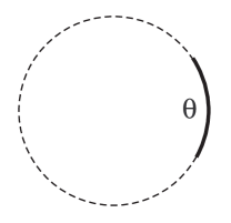
Figure 1: The arc containing the true points.

Next, assume for simplicity that the true points are equally spaced on an arc of size $\theta$ (a typical arrangement in many studies). Choosing the coordinate system so that the east pole $(1,0)$ is at the center of that arc (see Figure 1) ensures $\bar{y}=\overline{xy}=0$. It is not hard to see now that

(97) $$\tilde{\mathbf{M}}^{-}[1,0,0,0]^{T}=\tfrac{1}{4}(\overline{xx}-\bar{x}^{2})^{-1}[\overline{xx},-2\bar{x},0,\overline{xx}]^{T}.$$

Using the formula (88) we obtain (omitting details as they are not so relevant) the essential bias of the Kåsa fit in the natural parameters $(a,b,R)$:

(98) $${\mathbb{E}}(\Delta_{2}\hat{{\boldsymbol{\Theta}}}_{\rm Kasa})\stackrel{{\scriptstyle\rm ess}}{{=}}2\sigma^{2}\bigl{[}0,0,1\bigr{]}^{T}\,-\,\frac{\sigma^{2}}{\overline{xx}-\bar{x}^{2}}\bigl{[}-\bar{x},0,\overline{xx}\bigr{]}^{T}.$$

The first term here is the same as in (95) (recall that $\tilde{R}=1$), but it is the second term above that causes serious trouble: it grows to infinity because $\overline{xx}-\bar{x}^{2}\to 0$ as $\theta\to 0$. This explains why the Kåsa fit develops a heavy bias toward smaller circles when data points are sampled from a small arc.

9 Experimental tests and conclusions

To illustrate our analysis of various circle fits we have run a few computer experiments where we set $n$ true points equally spaced along a semicircle of radius $R=1$. Then we generated random samples by adding a Gaussian noise at level $\sigma=0.05$ to each true point, and after that applied various circle fits to estimate the parameters $(a,b,R)$.

	total MSE = variance + (ess. bias$)^{2}$ + rest of MSE
Pratt	$m$1.5164	$mm$1.2647	$mm$0.2500	$-$0.0017
Taubin	$m$1.3451	$mm$1.2647	$mm$0.0625	$-$0.0117
Geom.	$m$1.2952	$mm$1.2647	$mm$0.0156	$-$0.0149
Hyper.	$m$1.2892	$mm$1.2647	$mm$ 0.0000	$-$0.0244

Table 2: Mean square error (and its components) for four circle fits ($10^{4}\times$values are shown). In this test $n=100$ points are placed (equally spaced) along a semicircle of radius $R=1$ and the noise level is $\sigma=0.05$.

Table 2 summarizes the results of the first test, with $n=100$ points; it shows the mean square error (MSE) of the radius estimate $\hat{R}$ for each circle fit (obtained by averaging over $10^{7}$ randomly generated samples). The table also gives the breakdown of the MSE into three components. The first two are the variance (to the leading order) and the square of the essential bias, both computed according to our theoretical formulas. These two components do not account for the entire mean square error, due to higher order terms which our analysis discarded. The remaining part of the MSE is shown in the last column, which is relatively small. (We note that only the total MSE can be observed in practice; all the other columns of this table are the results of our theoretical analysis.)

We see that all the circle fits have the same (leading) variance, which accounts for the ‘bulk’ of the MSE. Their essential bias is different, it is highest for the Pratt fit and smallest (zero) for the Hyper fit. Algorithms with smaller essential biases perform overall better, i.e. have smaller mean square error. The Hyper fit is the best in our experiment; it outperforms the (usually unbeatable) geometric fit.

	total MSE = variance + (ess. bias$)^{2}$ + rest of MSE
Pratt	$m$25.5520	$mm$1.3197	$mm$25.0000	$-$-0.76784
Taubin	$m$7.4385	$mm$1.3197	$mm$6.2500	$-$-0.13126
Geom.	$m$2.8635	$mm$1.3197	$mm$1.5625	$-$-0.01876
Hyper.	$m$1.3482	$mm$1.3197	$mm$ 0.0000	$-$-0.02844

Table 3: Mean square error (and its components) for four circle fits ($10^{6}\times$values are shown). In this test $n=10000$ points are placed (equally spaced) along a semicircle of radius $R=1$ and the noise level is $\sigma=0.05$.

To highlight the superiority of the Hyper fit, we repeated our experiment increasing the sample up to $n=10000$, see Table 3 and Figure 2. We see that when the number of points is high, the the Hyper fit becomes several times more accurate than the geometric fit. Thus, our analysis disproves the popular belief in the statistical community that there is nothing better than minimizing the orthogonal distances.

Needless to say, the geometric fit involves iterative approximations, which are computationally intensive and subject to occasional divergence, while our Hyper fit is a fast non-iterative procedure, which is 100% reliable.

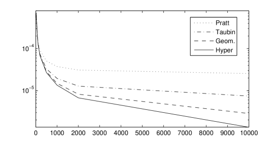
Figure 2: MSE for various circle fits (on the logarithmic scale) versus the sample size $n$ (from 10 to $10^{4}$).

Summary. All the known circle fits (geometric and algebraic) have the same variance, to the leading order. The relative difference between them can be traced to higher order terms in the expansion for the mean square error. The second leading term in that expansion is the essential bias, for which we have derived explicit expressions. Circle fits with smaller essential bias perform better overall. This explains a poor performance of the Kåsa fit, a moderate performance of the Pratt fit, and a good performance of the Taubin and geometric fits (in this order). We showed that while there is a natural lower bound on the variance to the leading order (the KCR bound), there is no lower bound on the essential bias. In fact there exists an algebraic fit with zero essential bias (the Hyper fit), which outperforms the geometric fit in accuracy. We plan to perform a similar analysis for ellipse fitting algorithms in the near future.

The authors are grateful to the anonymous referees for many helpful suggestions. N.C. was partially supported by National Science Foundation, grant DMS-0652896.

References

- [1] Y. Amemiya and W. A. Fuller. Estimation for the nonlinear functional relationship. Annals Statist., 16:147–160, 1988.
- [2] T. W. Anderson. Estimation of linear functional relationships: Approximate distributions and connections with simultaneous equations in econometrics. J. R. Statist. Soc. B, 38:1–36, 1976.
- [3] T. W. Anderson and T. Sawa. Exact and approximate distributions of the maximum likelihood estimator of a slope coefficient. J. R. Statist. Soc. B, 44:52–62, 1982.
- [4] A. Atieg and G. A. Watson. Fitting circular arcs by orthogonal distance regression. Appl. Numer. Anal. Comput. Math., 1:66–76.
- [5] M. Berman. Large sample bias in least squares estimators of a circular arc center and its radius. CVGIP: Image Understanding, 45:126–128, 1989.
- [6] N. N. Chan. On circular functional relationships. J. R. Statist. Soc. B, 27:45–56, 1965.
- [7] N. Chernov. Fitting circles to scattered data: parameter estimates have no moments. Manuscript, see http://www.math.uab.edu/ chernov/cl.
- [8] N. Chernov and C. Lesort. Statistical efficiency of curve fitting algorithms. Comp. Stat. Data Anal., 47:713–728, 2004.
- [9] N. Chernov and C. Lesort. Least squares fitting of circles. J. Math. Imag. Vision, 23:239–251, 2005.
- [10] N. Chernov and P. Sapirstein. Fitting circles to data with correlated noise. Comput. Statist. Data Anal., 52:5328–5337, 2008.
- [11] P. Delogne. Computer optimization of Deschamps’ method and error cancellation in reflectometry. In Proc. IMEKO-Symp. Microwave Measurement (Budapest), pages 117–123, 1972.
- [12] W. A. Fuller. Measurement Error Models. L. Wiley & Son, New York, 1987.
- [13] W. Gander, G. H. Golub, and R. Strebel. Least squares fitting of circles and ellipses. BIT, 34:558–578, 1994.
- [14] http://www.math.uab.edu/ chernov/cl.
- [15] S. H. Joseph. Unbiased least-squares fitting of circular arcs. Graph. Mod. Image Process., 56:424–432, 1994.
- [16] J. B. Kadane. Testing overidentifying restrictions when the disturbances are small. J. Amer. Statist. Assoc., 65:182–185, 1970.
- [17] K. Kanatani. Statistical Optimization for Geometric Computation: Theory and Practice. Elsevier Science, Amsterdam, Netherlands, 1996.
- [18] K. Kanatani. Cramer-Rao lower bounds for curve fitting. Graph. Mod. Image Process., 60:93–99, 1998.
- [19] K. Kanatani. For geometric inference from images, what kind of statistical model is necessary? Syst. Comp. Japan, 35:1–9, 2004.
- [20] K. Kanatani. Optimality of maximum likelihood estimation for geometric fitting and the KCR lower bound. Memoirs Fac. Engin. Okayama Univ., 39:63–70, 2005.
- [21] K. Kanatani. Ellipse fitting with hyperaccuracy. IEICE Trans. Inform. Syst., E89-D:2653–2660, 2006.
- [22] K. Kanatani. Statistical optimization for geometric fitting: Theoretical accuracy bound and high order error analysis. Int. J. Computer Vision, 80:167–188, 2008.
- [23] I. Kåsa. A curve fitting procedure and its error analysis. IEEE Trans. Inst. Meas., 25:8–14, 1976.
- [24] U. M. Landau. Estimation of a circular arc center and its radius. CVGIP: Image Understanding, 38:317–326, 1987.
- [25] P. Meer. Robust techniques for computer vision. In G. Medioni and S. B. Kang, editors, Emerging Topics in Computer Vision, pages 107–190. Prentice Hall, 2004.
- [26] Y. Nievergelt. A finite algorithm to fit geometrically all midrange lines, circles, planes, spheres, hyperplanes, and hyperspheres. J. Numerische Math., 91:257–303, 2002.
- [27] V. Pratt. Direct least-squares fitting of algebraic surfaces. Computer Graphics, 21:145–152, 1987.
- [28] C. Rusu, M. Tico, P. Kuosmanen, and E. J. Delp. Classical geometrical approach to circle fitting – review and new developments. J. Electron. Imaging, 12:179–193, 2003.
- [29] B. Sarkar, L. K. Singh, and D. Sarkar. Approximation of digital curves with line segments and circular arcs using genetic algorithms. Pattern Recogn. Letters, 24:2585–2595, 2003.
- [30] H. Späth. Least-squares fitting by circles. Computing, 57:179–185, 1996.
- [31] A. Strandlie, J. Wroldsen, R. Frühwirth, and B. Lillekjendlie. Particle tracks fitted on the Riemann sphere. Computer Physics Commun., 131:95–108, 2000.
- [32] G. Taubin. Estimation of planar curves, surfaces and nonplanar space curves defined by implicit equations, with applications to edge and range image segmentation. IEEE Trans. Pattern Analysis Machine Intelligence, 13:1115–1138, 1991.
- [33] D. Umbach and K. N. Jones. A few methods for fitting circles to data. IEEE Trans. Instrument. Measur., 52:1181–1885, 2003.
- [34] K. M. Wolter and W. A. Fuller. Estimation of nonlinear errors-in-variables models. Annals Statist., 10:539–548, 1982.
- [35] S. J. Yin and S. G. Wang. Estimating the parameters of a circle by heteroscedastic regression models. J. Statist. Planning Infer., 124:439–451, 2004.
- [36] E. Zelniker and V. Clarkson. Maximum-likelihood estimation of circle parameters via convolution. IEEE Trans. Image Proc., 15:865–876, 2006.
- [37] E. Zelniker and V. Clarkson. A statistical analysis of the Delogne-Kåsa method for fitting circles. Digital Signal Proc., 16:498–522, 2006.
- [38] S. Zhang, L. Xie, and M. D. Adams. Feature extraction for outdoor mobile robot navigation based on a modified gauss newton optimization approach. Robotics Autonom. Syst., 54:277–287, 2006.