Bounding the Probability of Error for High Precision Recognition

Abstract

We consider models for which it is important, early in processing, to estimate some variables with high precision, but perhaps at relatively low rates of recall. If some variables can be identified with near certainty, then they can be conditioned upon, allowing further inference to be done efficiently. Specifically, we consider optical character recognition (OCR) systems that can be bootstrapped by identifying a subset of correctly translated document words with very high precision. This “clean set” is subsequently used as document-specific training data. While many current OCR systems produce measures of confidence for the identity of each letter or word, thresholding these confidence values, even at very high values, still produces some errors.

We introduce a novel technique for identifying a set of correct words with very high precision. Rather than estimating posterior probabilities, we bound the probability that any given word is incorrect under very general assumptions, using an approximate worst case analysis. As a result, the parameters of the model are nearly irrelevant, and we are able to identify a subset of words, even in noisy documents, of which we are highly confident. On our set of 10 documents, we are able to identify about 6% of the words on average without making a single error. This ability to produce word lists with very high precision allows us to use a family of models which depends upon such clean word lists.

1 Introduction

The goal of this paper is to post-process the output from an optical character recognition (OCR) program and identify a list of words which the program got correct. The motivation is to use these correct words to build new OCR models based upon training data from the document itself, i.e., to build a document-specific model.

In this paper, we focus on the first step–identifying the correct words in someone else’s OCR program output. While this may seem like an easy thing to do, to our knowledge, there are no existing techniques to perform this task with very high accuracy. There are many methods that could be used to produce lists of words that are mostly correct, but contain some errors. Unfortunately, such lists are not much good as training data for document-specific models since they contain errors, and these errors in training propagate to create more errors later.

Thus, it is essential that our error rate be very low in the list of words we choose as correct. As described below, we do not in fact make any errors at all in our generated lists, which makes them appropriate for training document specific models. Before going into the details of our method and how we achieve an empirical error rate of 0% for this task, we give some background on why we believe this problem and our approach are interesting.

2 Background

Humans and machines both make lots of errors in recognition problems. However, one of the most interesting differences between people and machines is that, for some inputs, humans are extremely confident of their results and appear to be well-justified in this confidence. Machines, on the other hand, while producing numbers such as posterior probabilities which are supposed to represent confidences, are often wrong even when posterior probabilities are extremely close to 1.

This is a particularly vexing problem when using generative models in areas like computer vision and pattern recognition. Consider a two class problem in which we are discriminating between two similar image classes, $A$ and $B$. Because images are so high-dimensional, likelihood exponents are frequently very small, and small errors in these exponents can render the posteriors meaningless. For example, suppose that $Pr(\tt{image}|A)=\exp(-1000+\epsilon_{A})$ and $Pr(\tt{image}|B)=\exp(-1005+\epsilon_{B})$, where $\epsilon_{A}$ and $\epsilon_{B}$ represent errors in the estimates of the image distributions. Assuming an equal prior on $A$ and $B$, if $\epsilon_{A}$ and $\epsilon_{B}$ are Gaussian distributed with standard deviation similar to the differences in the exponents, then we will frequently conclude, incorrectly, that $Pr(B|\tt{image})\approx 1$ and $Pr(A|\tt{image})\approx 0$. This phenomenon, which is quite common in computer vision, makes it quite difficult to assess confidence values in recognition problems.

As an alternative to estimating posterior probabilities very accurately in order to be sure of certain results, we suggest an alternative. We formulate our confidence estimate as an hypothesis test that a certain result is incorrect, and if there is sufficient evidence, we reject the hypothesis that the result is incorrect. As we shall see, this comes closer to bounding the probabilities of certain results, which can be done with greater confidence, than estimating the probability of results, which is much more difficult. A critical aspect of our approach is that if there is insufficient evidence to reject a hypothesis, then we make no decision at all. Our process only makes decisions when there is enough evidence, and avoids making decisions when there is not. More formally, we search for cases in which our conservative bounds on the probability of error are non-vacuous–if they are vacuous, we make no decision.

2.1 OCR and Document Specific Modeling

Despite claims to the contrary, getting OCR systems to obtain very high accuracy rates on moderately degraded documents continues to be a challenging problem [24]. One promising approach to achieving very high OCR accuracy rates is to incorporate document specific modeling [13, 16, 17]. This set of approaches attempts to refine OCR models to specifically model the document currently being processed by adapting to the fonts in the document, adapting to the noise model in the document, or adapting to the lexicon in the document.

If one had some method for finding a sample of words in a document which were known to be correct with high confidence, one could effectively use the characters in such words as training data with which to build document specific models of the fonts in a document. This chicken-and-egg problem is not easy to solve, however. Our main result in this paper is to present a method for post-processing third party OCR outputs, in moderately difficult documents, to produce lists of words that are 100% correct. As a comparison with our results, we do experiments using a public domain OCR system that maintains a built-in confidence measure for its own outputs. We show that there is no threshold on this confidence value that produces clean word lists for most documents without either an unacceptably small number of correct words (usually 0), or an unacceptably large percentage of errors.

In this paper, we consider a completely new approach to obtaining a “clean word list” for document specific modeling. Rather than trying to estimate the probability that an intermediate output of an OCR system (like an HMM or CRF) is correct and then thresholding this probability, we instead form a set of hypotheses about each word in the document. Each hypothesis poses that one particular word of the first-pass OCR system is incorrect. We then search for hypotheses that we can reject with high confidence. More formally, we treat a third party OCR system (in this case, the open source OCR program Tesseract [1]) as a null hypothesis generator, in which each attempted transcription $T$ produced by the OCR system is treated as the basis for a separate null hypothesis. The null hypothesis for word $T$ is simply “Transcription $T$ is incorrect.”. Letting $W$ be the true identity of a transcription $T$, we notate this as

$$T\neq W.$$

Our goal is to find as many hypotheses as possible that can be rejected with high confidence. For the purposes of this paper, we take high confidence to mean with fewer than 1 error in a million rejected hypotheses. Since we will only be attempting to reject a few hundred hypotheses, this implies we shouldn’t make any errors at all. As our results section shows, we do not make any errors in our clean word lists, even when they come from quite challenging documents.

Before proceeding, we stress that the following are not goals of this paper:

• to present a complete system for OCR,

• to produce high area under a precision recall curve for all of the words in a document,

• to produce accurate estimates of the probability of error of particular words in OCR.

Once again, our goal is simply to produce large lists of clean words from OCR output so that we can use them for document-specific modeling. After presenting our method for producing clean word lists, we provide a formal analysis of the bounds on the probability of incorrectly including a word in our clean word list, under certain assumptions. When our assumptions hold, our error bound is very loose, meaning our true probability of error is much lower. However, some documents do in fact violate our assumptions. Finally, we give an example of what can be done with the clean word lists by showing some simple error correction results on a real-world OCR problem.

3 Method for Producing Clean Word Lists

In this section, we present our method for taking a document and the output of an OCR system and producing a so-called clean word list, i.e. a list of words which we believe to be correct, with high confidence. Our success will be measured by the number of words that can be produced, and whether we achieve a very low error rate. A priori, we decided that our method would be a failure if it produced more than a single error per document processed. To be a success, we must produce a clean word list which is long enough to produce an interesting amount of training data for document-specific processing.

We assume the following setup.

• We are provided with a document $D$ in the form of a grayscale image.

• We are provided with an OCR program. From here forward, we will use the open source OCR program Tesseract as our default OCR program.

• We further assume that the OCR program can provide an attempted segmentation of the document $D$ into words, and that the words are segmented into characters. It is not necessary that the segmentation be entirely correct, but merely that the program produces an attempted segmentation.

• In addition to a segmentation of words and letters, the program should produce a best guess for every character it has segmented, and hence, by extension, of every word (or string) it has segmented. Of course, we do not expect all of the characters or words to be correct, as that would make our exercise pointless.

• Using the segmentations provided by the OCR program, we assume we can extract the gray-valued bitmaps representing each guessed character from the original document.

• Finally, we assume we are given a lexicon. Our method is relatively robust to the choice of lexicon, and assumes there will be a significant number of non-dictionary words.

We define a few terms before proceeding. We define the Hamming distance between two strings of the same number of characters to be the number of character substitutions necessary to convert one string to the other. We define the Hamming ball of radius $r$ for a word $W$, $H_{r}(W)$, to be the set of strings whose Hamming distance to $W$ is less than or equal to $r$. Later, after defining certain equivalence relationships among highly confusable characters such as “o” and “c”, we define a pseudo-Hamming distance which is equivalent to the Hamming distance except that it ignores substitutions among characters in the same equivalence class. We also use the notions of edit distance, which extends Hamming distance by including joins and splits of characters, and pseudo-edit distance, which is edit distance using the aforementioned equivalence classes.

Our method for identifying words in the clean list has three basic steps. We consider each word $T$ output by Tesseract.

1. First, if $T$ is not a dictionary word, we discard it and make no attempt to classify whether it is correct. That is, we will not put it on the clean word list.

2. Second, given that $T$ is a dictionary word, we evaluate whether $H_{1}(T)$ is non-empty, i.e. whether there are any dictionary words for which a single change of a letter can produce another dictionary word. If so, we discard the word, and again make no attempt to classify whether it is correct.

3. Assuming we have passed the first two tests, we now perform a consistency check (described below) of each character in the word. If the consistency check is passed, we declare the word to be correct.

Consistency check

In the following, we refer to the bitmap associated with a character whose identity is unknown as a glyph. Let $W_{j}$ be the true character class of the $j$th glyph of a word $W$, and let $T_{j}$ be the Tesseract interpretation of the same glyph. The goal of a consistency check is to try to ensure that the Tesseract interpretation of a glyph is reliable. We will assess reliability by checking whether other similar glyphs usually had the same interpretation by Tesseract.

To understand the purpose of the consistency check, consider the following situation. Imagine that a document had a stray mark that did not look like any character at all, but was interpreted by Tesseract as a character. If Tesseract thought that the stray mark was a character, it would have to assign it to a character class like “t”. We would like to detect that this character is unreliable. Our scheme for doing this is to find other characters that are similar to this glyph, and to check the identity assigned to those characters by Tesseract. If a large majority of those characters are given the same interpretation by Tesseract, then we consider the original character to be reliable. Since it is unlikely that the characters closest to the stray mark are clustered tightly around the true character “t”, we hope to detect that the stray mark is atypical, and hence unreliable.

More formally, to test a glyph $g$ for reliability, we first find the $M$ characters in the document that are most similar to $g$. We then run the following procedure:

• Step 1. Initialize $i$ to 1.

• Step 2. Record the class of the character that is $i$th most similar to $g$. We use normalized correlation as a similarity measure.

• Step 3. If any character class $c$ has matched $g$ a number of times $c_{n}$ such that $\frac{c_{n}}{i+1}>\theta$, then declare the character $g$ to be $\theta$-dominated by the class $c$, and terminate the procedure.

• Step 4. Otherwise, add 1 to i. If $i<M$, go to Step 2.

• Step 5. If, after the top $M$ most similar characters to $g$ are evaluated, no character class $c$ dominates the glyph, then we declare that the glyph $g$ is undominated.

There are three possible outcomes of the consistency check. The first is that the glyph $g$ is dominated by the same class $c$ as the Tesseract interpretation of $g$, namely $T_{j}$. The second outcome is that $g$ is dominated by some other class that does not match $T_{j}$. The third outcome is that $g$ is undominated. In the latter two cases, we declare the glyph $g$ to be unreliable. Only if the glyph $g$ is dominated by the same class as the Tesseract identity of $g$ do we declare $g$ to be reliable. Furthermore, only if all of the characters in a word are reliable do we declare the word to be reliable or “clean”.

The constants used in our experiments were $M=20$ and $\theta=0.66$. That is, we compared each glyph against a maximum of 20 other glyphs in our reliability check, and we insisted that a “smoothed” estimate of the number of similarly interpreted glyphs was at least 0.66% before declaring a character to be reliable. We now analyze the probability of making an error in the clean set.

4 Theoretical bound

For a word in a document, let $W$ be the ground truth label of the word, $T$ be the Tesseract labeling of the word, and $C$ be a binary indicator equal to 1 if the word passed the consistency check. We want to upper bound the probability $\Pr(W\neq w_{t}|T=w_{t},C=1)$ when $w_{t}$ is a dictionary word and has an empty Hamming ball of size 1.

$$\Pr(W\neq w_{t}|T=w_{t},C=1) = \sum_{w\neq w_{t}}\Pr(W=w|T=w_{t},C=1)$$ (1)

$$= \sum_{w\neq w_{t},w\in\text{Dict}}\Pr(W=w|T=w_{t},C=1)$$

$$+\sum_{w\neq w_{t},w\notin\text{Dict}}\Pr(W=w|T=w_{t},C=1)$$

$$= \sum_{w\neq w_{t},w\in\text{Dict},|w|=|w_{t}|}\Pr(W=w|T=w_{t},C=1)$$

$$+\sum_{w\neq w_{t},w\in\text{Dict},|w|\neq|w_{t}|}\Pr(W=w|T=w_{t},C=1)$$

$$+\sum_{w\neq w_{t},w\notin\text{Dict}}\Pr(W=w|T=w_{t},C=1)$$

4.1 Bounding the character consistency check

We will rewrite the $\Pr(W=w|T=w_{t},C=1)$ terms as bounds involving $\Pr(C=1|T=w_{t},W=w)$ using Bayes’ Rule. We will make the assumption that the individual character consistency checks are independent, although this is not exactly true, since there may be local noise that degrades characters in a word in the same way.

Assume that each character is formed on the page by taking a single true, latent appearance based on the font and the particular character class and adding some amount of noise. Let $\epsilon$ be an upper bound on the probability that noise has caused a character of any given class to look like it belongs to another specific class other than its own class. More formally, letting $p_{c}(a)$ be the probability of a character appearance $a$ for a given class $c$ under the noise model, $\epsilon$ satisfies, for all character classes $c_{1},c_{2},c_{1}\neq c_{2}$,

$$\epsilon > \int_{a|p_{c_{1}}(a)<p_{c_{2}}(a)}p_{c_{1}}(a)da.$$ (4)

In order to obtain a small value for $\epsilon$, and hence later a small probability of error, we revise Eq. 4 to be a bound only on non-confusable character classes. In other words, since some character classes are highly confusable, such as ’o’, ’c’, and ’e’, we ignore such substitutions when computing Hamming and edit distance. We’ll refer to these distances as modified distances, so mode and mere have a true Hamming distance of 2 but a modified Hamming distance of 1.

This is similar to defining an equivalence relation where confusable characters belong to the same equivalence class, and computing distance over the quotient set, but without transitivity, as, for example, ’h’ may be confusable with ’n’, and ’n’ may be confusable with ’u’, but ’h’ may not necessarily be confusable with ’u’.

For a character to pass a consistency check with the label $c_{2}$ when the true underlying label is $c_{1}$, roughly one of two things must happen: (a) either the character was corrupted and looked more like $c_{2}$ than $c_{1}$, or (b) some number of other characters with label $c_{2}$ were corrupted and looked like $c_{1}$’s.

The probability (a) is clearly upper bounded by $\epsilon$, since it requires both the corruption and most of its neighbors to have the same label $c_{2}$. Since $\epsilon\ll 1$ and (b) requires several other characters with label $c_{2}$ to be corrupted to look like $c_{1}$, the probability of (b) should be bounded by (a), and thus $\epsilon$, as well.

Therefore the probability of the consistency check giving a label $c_{2}$ when the true underlying label is $c_{1}$ is less than $2\epsilon$, for any classes $c_{1},c_{2}$.

We will also need a lower bound on the probability that a character consistency check will succeed if the Tesseract label of the character matches the ground truth label. Let $\delta$ be a lower bound on this quantity, which is dependent on both the amount of noise in the document and the length of the document. (The latter condition is due to the fact that the character consistency check requires a character to match to at least a certain number of other similarly labeled characters, so, for example, if that number isn’t present in the document to begin with, then the check will fail with certainty.)

4.2 Bounding one term

Consider, bounding $\Pr(W=w|T=w_{t},C=1)$:

$$\Pr(W=w|T=w_{t},C=1)$$

$$\qquad\qquad=\frac{\Pr(C=1|T=w_{t},W=w)\Pr(W=w|T=w_{t})}{\sum_{w^{\prime}}\Pr(C=1|T=w_{t},W=w^{\prime})\Pr(W=w^{\prime}|T=w_{t})}$$ (5)

$$\qquad\qquad=\frac{\Pr(C=1|T=w_{t},W=w)\Pr(T=w_{t}|W=w)\Pr(W=w)}{\sum_{w^{\prime}}\Pr(C=1|T=w_{t},W=w^{\prime})\Pr(T=w_{t}|W=w^{\prime})\Pr(W=w^{\prime})}$$ (6)

$$\qquad\qquad\leq\frac{\Pr(C=1|T=w_{t},W=w)\Pr(T=w_{t}|W=w)\Pr(W=w)}{\Pr(C=1|T=w_{t},W=w_{t})\Pr(T=w_{t}|W=w_{t})\Pr(W=w_{t})}$$ (7)

4.3 Bounding dictionary words

For dictionary words $w$, we will assume that

$$\frac{\Pr(T=w_{t}|W=w)\Pr(W=w)}{\Pr(T=w_{t}|W=w_{t})\Pr(W=w_{t})} < 1,$$ (8)

or, equivalently,

$$\frac{\Pr(W=w|T=w_{t})}{\Pr(W=w_{t}|T=w_{t})} < 1.$$ (9)

Eq. 8 can be thought of as balance between Tesseract’s word level accuracy $\frac{\Pr(T=w_{t}|W=w)}{\Pr(T=w_{t}|W=w_{t})}$ and the words’ prior probabilities $\frac{\Pr(W=w)}{\Pr(W=w_{t})}$. In our documents, word level accuracy $\Pr(T=w_{t}|W=w_{t})$ is generally around .9, and the numerator in the first ratio $\Pr(T=w_{t}|W=w)$ is the probability of Tesseract making a specific mislabeling, and so is upper bounded by .1 but generally will be much lower.

Applying this to Eq. 7, we get

$$\Pr(W=w|T=w_{t},C=1) \leq \frac{\Pr(C=1|T=w_{t},W=w)}{\Pr(C=1|T=w_{t},W=w_{t})}.$$ (10)

4.3.1 Bounding dictionary Hamming words

Consider a word $w$ that is a modified Hamming distance $i$ from $w_{t}$. We can then simplify Eq. 10 as

$$\Pr(W=w|T=w_{t},C=1) \leq \frac{(2\epsilon)^{i}}{\delta^{i}}$$ (11)

by making use of the assumption that the character consistency checks are independent, and that $w$ and $w_{t}$ only differ in $i$ characters. For those $i$ characters, $w$ does not match the Tesseract label and $w_{t}$ does match the Tesseract label, so we use the bounds $2\epsilon$ and $\delta$.

Now let $D_{i}$ be the number of dictionary words of modified Hamming distance $i$ away from $w_{t}$. Let $r_{D}$ be the rate of growth of $D_{i}$ as a function of $i$, e.g. $D_{i+2}=r_{D}^{i}D_{2}$. Assume, since $\epsilon\ll 1$, that $r_{D}(\frac{2\epsilon}{\delta})<\frac{1}{2}$. (Experiments on the dictionary used in our main experiments showed that $r_{D}$ is generally about 3.)

To get the total contribution to the error from all dictionary Hamming words, we sum over $D_{i}$ for all $i>1$,

$$\sum_{w\neq w_{t},w\in\text{Dict},|w|=|w_{t}|}\Pr(W=w|T=w_{t},C=1) \leq \sum_{i=2}D_{i}\frac{(2\epsilon)^{i}}{\delta^{i}}$$ (12)

$$= D_{2}\frac{(2\epsilon)^{2}}{\delta^{2}}+D_{2}\frac{(2\epsilon)^{2}}{\delta^{2}}\sum_{i=1}(2r_{D}\frac{\epsilon}{\delta})^{i}$$ (13)

$$\leq 8D_{2}\frac{\epsilon^{2}}{\delta^{2}}.$$ (14)

4.3.2 Bounding dictionary edit words

Traditionally, edit distance is computed in terms of number of substitutions, insertions, and deletions necessary to convert one string to another string. In our context, a more natural notion may be splits and joins rather than insertions and deletions. For example, the interpretation of an ’m’ may be split into an ’r’ and a ’n’, or vice-versa for a join.

The probability that a split or a join passes the consistency check is upper bounded by $(2\epsilon)^{2}$. We can see this from two perspectives. First, a split or join has traditional edit distance of 2, since it requires an insertion or deletion and a substitution (’m’ to ’mn’ insertion followed by ’mn’ to ’rn’ substitution).

A more intuitive explanation is that, for a split, one character must be corrupted to look like the left hand side of the resulting character and another character corrupted to look like the right hand side, and for a join, the left hand side of a character must be corrupted to look like one character and the right hand side corrupted to look like another.

Similar to the case of confusable characters for substitutions, we also ignore confusable characters for splits and joins, namely ’r’ followed by ’n’ with ’m’, and ’v’ followed by ’v’ with ’w’. Thus, corn and comb have an edit distance of 2 but a modified edit distance of 1.

Consider a word $w$ with modified edit distance $i$ from $w_{t}$, and involving at least one insertion or deletion (so $|w|\neq|w_{t}|$). Similar to the dictionary Hamming words, we can simplify Eq. 10 for $w$ as

$$\Pr(W=w|T=w_{t},C=1) \leq \frac{(2\epsilon)^{i+1}}{\delta^{i}},$$ (15)

since each substitution contributes a $\frac{2\epsilon}{\delta}$ and each insertion or deletion, of which there is at least one, contributes a $\frac{(2\epsilon)^{2}}{\delta}$.

Let $E_{i}$ be the number of dictionary words $w$ with a modified edit distance $i$ away from $w_{t}$ and $|w|\neq|w_{t}|$.

Again, also assume that $r_{E}$, the rate of growth of $E_{i}$, satisfies $r_{E}(\frac{2\epsilon}{\delta})<\frac{1}{2}$. Summing the total contribution to the error from dictionary edit words,

$$\sum_{w\neq w_{t},w\in\text{Dict},|w|\neq|w_{t}|}\Pr(W=w|T=w_{t},C=1) \leq \sum_{i=1}E_{i}\frac{(2\epsilon)^{i+1}}{\delta^{i}}$$ (16)

$$= E_{1}\frac{(2\epsilon)^{2}}{\delta}+E_{1}\frac{(2\epsilon)^{2}}{\delta}\sum_{i=1}(2r_{E}\frac{\epsilon}{\delta})^{i}$$ (17)

$$\leq 8E_{1}\frac{\epsilon^{2}}{\delta}$$ (18)

$$\leq 8E_{1}\frac{\epsilon^{2}}{\delta^{2}}.$$ (19)

4.4 Bounding non-dictionary words

Let $N_{i}$ be the set of non-dictionary words with a modified edit distance $i$ from $w_{t}$, and let $p_{i}=\frac{\Pr(T=w_{t}|W\in N_{i})\Pr(W\in N_{i})}{\Pr(T=w_{t}|W=w_{t})\Pr(W=w_{t})}$. Assume the rate of growth of $r_{N}$ of $p_{i}$ satisfies $r_{N}(\frac{2\epsilon}{\delta})<\frac{1}{2}$.

Rearranging Eq. 7 and summing over all non-dictionary words:

$$\sum_{w\neq w_{t},w\notin\text{Dict}}\Pr(W=w|T=w_{t},C=1)$$

$$\qquad\qquad\leq\sum_{i=1}\sum_{w\in N_{i}}\frac{\Pr(C=1|T=w_{t},W=w)\Pr(W=w|T=w_{t})}{\Pr(C=1|T=w_{t},W=w_{t})\Pr(W=w_{t}|T=w_{t})}$$ (20)

$$\qquad\qquad\leq\sum_{i=1}\sum_{w\in N_{i}}\frac{(2\epsilon)^{i}}{\delta^{i}}\frac{\Pr(W=w|T=w_{t})}{\Pr(W=w_{t}|T=w_{t})}$$ (21)

$$\qquad\qquad=\sum_{i=1}\frac{(2\epsilon)^{i}}{\delta^{i}}\frac{\Pr(W\in N_{i}|T=w_{t})}{\Pr(W=w_{t}|T=w_{t})}$$ (22)

$$\qquad\qquad=\sum_{i=1}\frac{(2\epsilon)^{i}}{\delta^{i}}p_{i}$$ (23)

$$\qquad\qquad\leq p_{1}\frac{2\epsilon}{\delta}+p_{1}\frac{2\epsilon}{\delta}\sum_{i=1}(2r_{N}\frac{\epsilon}{\delta})^{i}$$ (24)

$$\qquad\qquad\leq 4p_{1}\frac{\epsilon}{\delta^{2}}$$ (25)

4.5 Final bound

$$\Pr(W\neq w_{t}|T=w_{t},C=1) \leq \frac{(8D_{2}+8E_{1})\epsilon^{2}+4p_{1}\epsilon}{\delta^{2}}$$ (26)

For $\epsilon<10^{-3}$, $8D_{2}+8E_{1}<10^{2}$, $4p_{1}<10^{-1}$, $\delta^{2}>10^{-1}$,

$$\Pr(W\neq w_{t}|T=w_{t},C=1) \leq 2\cdot 10^{-3}.$$ (27)

The bounds for the constants chosen above were selected conservatively to hold for a large range of documents, from very clean to moderately noisy. Not all documents will necessarily satisfy these bounds. In a sense, these inequalities define the set of documents for which our algorithm is expected to work, and for heavily degraded documents that fall outside this set, the character consistency checks may no longer be robust enough to guarantee a very low probability of error.

Our final bound on the probability of error, 0.002, is the result of a worst case analysis under our assumptions. If our assumptions hold, the probability of error will likely be much lower for the following reasons. For most pairs of letters, $\epsilon=10^{-3}$ is not a tight upper bound. The quantity on the right of Eq. 8 is typically much lower than 1. The rate of growths $r_{D},r_{E},r_{N}$ are typically much lower than assumed. The bound on $p_{1}$, the non-dictionary word probabilities, is not a tight upper bound, as non-dictionary words mislabeled as dictionary words are rare. Finally, the number of Hamming and edit distance neighbors $D_{2}$ and $E_{1}$ will typically be less than assumed.

On the other hand, for sufficiently noisy documents, and certain types of errors, our assumptions do not hold. Some of the problematic cases include the following. As discussed, the assumption that the individual character consistency checks are independent is not true. If a document is degraded or has a font such that one letter is consistently interpreted as another, then that error will likely pass the consistency check (e.g. $\epsilon$ will be very large). If a document is degraded or is very short, then $\delta$ may be much smaller than $10^{-\frac{1}{2}}$. (The character consistency check requires a character to match to at least a certain number of other similarly labeled characters, so, for example, if that number isn’t present in the document to begin with, then the check will fail with certainty.) Finally, if the dictionary is not appropriate for the document then $4p_{1}<10^{-1}$ may not hold. This problem is compounded if the OCR system projects to dictionary words.

5 Experiments

We analyzed 10 short documents (4-5 pages each) with Tesseract word accuracy rates between 58% and 95% (see Table 1) [22, 2, 3, 12, 4, 5, 6, 7, 8, 9]. A portion of one document is shown in Figure 2. Note that in order to simulate document degradation, we downsampled some of the documents from the Project Gutenberg corpus.

Applying the method of Section 3, we produced “conservative” clean word lists as shown in Table 1. Our main result is that we are able to extract an average of 6% of the words in each document without making a single error. The total number of words in all of the conservative clean lists was 843, giving some informal support to the legitimacy of our bound, which suggests we would expect between 1 and 2 errors in a worst case scenario, and fewer than that under average conditions. We found that we could relax the requirement that a word have empty Hamming ball of radius 1 (Step 2 of our method) and replace it with a less stringent requirement, while only introducing a single error into what we called an “aggressive clean word list” (see Table 1). In particular, we replaced the empty Hamming ball requirement with a requirement that a word either have an empty Hamming ball of radius 1, or, if it had neighbors of Hamming distance 1, that those neighbors not occur elsewhere in the document. This less restrictive definition of the clean word sets, no longer subject to our analytic bound, produces much larger clean lists (2661 words) while producing just a single error.

Document	Word	Tesseract	Conservative List		Conserv.	Aggressive List		Aggress.
Name	Count	Accuracy	Count	%	Errors	Count	%	Errors
Archie	754	80.1%	29	3.8%	0	106	14.1%	0
Beauty	1706	86.1%	69	4.0%	0	308	18.1%	0
Campfire	711	64.3%	4	0.6%	0	27	3.8%	0
Cosmic	1533	86.6%	60	3.9%	0	222	14.5%	1
Country	892	58.3%	20	2.2%	0	92	10.3%	0
Cristo	886	86.7%	31	3.5%	0	136	15.3%	0
Geology	1498	95.2%	121	8.1%	0	392	26.2%	0
History	2712	79.7%	245	9.0%	0	571	21.1%	0
Mackay	2056	85.4%	175	8.5%	0	522	25.4%	0
Oahu	1309	88.9%	89	6.8%	0	285	21.8%	0
Totals	14057	82.9%	843	6.0%	0	2661	18.9%	1

Table 1: Results. Using our conservative clean list approach, we retrieved an average of 6% of the words in our test documents with 0 errors. Using our aggressive approach, we obtained an average of 18.9% with only a single error.

As mentioned in the introduction, many OCR programs come with some notion of a confidence estimate for each word or character that is produced. Tesseract has two separate functions which are related to its confidence of word accuracy. An obvious approach to producing clean word lists is to simply learn a threshold on the confidence values output by an OCR program.

Consider the heavy black line in Figure 1. This line shows the precision/recall curve for the words in all of our test documents together as the threshold on the Tesseract confidence value is changed. It is easy to see that there is no threshold of the confidence value that achives a word accuracy rate of higher than about 95%. Hence, there is no confidence level which can be used to produce clean word lists across all documents. The individual colored curves show precision/recall curves for individual documents. While there exist Tesseract confidence thresholds that produce error-free clean word lists for some documents, the same confidence levels do not work for other documents, showing, that as a general technique, using a threshold on the Tesseract confidence value cannot be used in a naive fashion to produce such clean word lists.

Finally, notice the black and red X’es at the top of the figure. The black X (on the left) represents the average recall rate of about 6% and the perfect precision of our conservative clean word generation scheme averaged across all documents. The red X (on the right) shows the slightly lower precision and significantly higher recall of our aggressive clean word generation scheme, again averaged across all documents.

5.1 Using the clean word sets

While it is not the main thrust of this paper, we have begun to experiment with using the clean word sets to improve OCR results. In our first experiment, we extract all examples of a pair of confusable characters (“o” and “c”) from the conservative list of the Mackay document. We then trained a linear support vector machine classifier on this list, and reclassified all instances of “o” and “c” not in the conservative list. While Tesseract made four errors confusing “o”s and “c”s in the original document, all of these were corrected using our document-specific training set, and no new errors were introduced. While this clearly represents just a beginning, we believe it is a promising sign that document specific training sets will be useful in correcting a variety of errors in OCR documents. It is interesting to note that no new data needed to be labeled for this experiment. Everything was done fully automatically.

Related work.

There has been significant work done in post-processing the output of OCR. While none of it is very similar to what we have presented here, we present some points of reference for completeness. Kolak et al. [19] developed a generative model to estimate the true word sequence from noisy OCR output and Kukich et al. [20] survey various methods to correct text using natural language processing techniques. Hong et al. [18] examine the inter-word relationships of character patches to help constrain possible interpretations. The distinguishing feature of our work is that we examine the document images themselves to build document-specific models of the characters.

Our work is also related to a variety of approaches that leverage inter-character similarity in documents in order to reduce the dependence upon a priori character models. Some of the most significant developments in this area are found in these papers [11, 10, 21, 23, 15, 14]. The inability to attain high confidence in either the identity or equivalence of characters in these papers has hindered their use in subsequent OCR developments. We hope that the high confidence values we obtained will spur the use of these techniques for document-specific modeling.

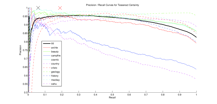
Figure 1: Precision recall curves using Tesseract’s confidence measure for individual documents (colored lines) and aggregate document (heavy black line). No threshold on the confidence measure produces satisfactory clean word lists. Our points on the precision recall curve are shown for our conservative procedure (black X on left) and our aggressive procedure (red X on right).

Figure 2: The top portion of page 2 of the Mackay document. Notice the degraded characters, which produces a significant number of errors in the Tesseract OCR program.

References

- [1] http://code.google.com/p/tesseract-ocr/.
- [2] http://www.gutenberg.org/etext/20809/.
- [3] http://www.gutenberg.org/etext/20669/.
- [4] http://www.gutenberg.org/etext/20713/.
- [5] http://www.gutenberg.org/etext/19967/.
- [6] http://www.gutenberg.org/etext/26216/.
- [7] http://www.gutenberg.org/etext/20719/.
- [8] From DOE Sample 3 Corpus. http://www.isri.unlv.edu/ISRI/OCRtk.
- [9] http://www.gutenberg.org/etext/20727/.
- [10] T.M. Breuel. Character recognition by adaptive statistical similarity. In ICDAR, 2003.
- [11] R.G. Casey. Text OCR by solving a cryptogram. In ICPR, 1986.
- [12] E. Colin Cherry. A history of the theory of information. Information Theory, Transaction of the IRE Professional Group, 1(1):33–36, 1953.
- [13] Tin Kam Ho. Bootstrapping text recognition from stop words. In Procs. ICPR-14, pages 605–609, 1998.
- [14] T.K. Ho and G. Nagy. OCR with no shape training. In ICPR, 2000.
- [15] J.D. Hobby and T.K. Ho. Enhancing degraded document images via bitmap clustering and averaging. In ICDAR, 1997.
- [16] T. Hong and J.J. Hull. Improving OCR performance with word image equivalence. In Symposium on Document Analysis and Information Retrieval, 1995.
- [17] T. Hong and J.J. Hull. Visual inter-word relations and their use in character segmentation. In SPIE, 1995.
- [18] Tao Hong and Jonathan J. Hull. Visual inter-word relations and their use in ocr post-processing. In Proceedings of the Third International Conference on Document Analysis and Recognition, pages 14–16, 1995.
- [19] Okan Kolak. A generative probabilistic ocr model for nlp applications. In In HLT-NAACL 2003, pages 55–62, 2003.
- [20] Karen Kukich. Techniques for automatically correcting words in text. ACM Comput. Surv., 24(4):377–439, 1992.
- [21] D. Lee. Substitution deciphering based on HMMs with applications to compressed document processing. IEEE Transactions on Pattern Analysis and Machine Intelligence, 24(12), 2002.
- [22] D.M. MacKay. Entropy, time and information (introduction to discussion). Information Theory, Transaction of the IRE Professional Group, 1(1):162–165, 1953.
- [23] G. Nagy. Efficient algorithms to decode substitution ciphers with applications to OCR. In ICPR, 1986.
- [24] G. Nagy. Twenty years of document image analysis in PAMI. IEEE Transactions on Pattern Analysis and Machine Intelligence, 22(1), 2000.