Transport and Strong-Correlation Phenomena in
Carbon Nanotube Quantum Dots in a Magnetic Field

Abstract

Transport through carbon nanotube (CNT) quantum dots (QDs) in a magnetic field is discussed. The evolution of the system from the ultraviolet to the infrared is analyzed; the strongly correlated (SC) states arising in the infrared are investigated. Experimental consequences of the physics are presented — the SC states arising at various fillings are shown to be drastically different, with distinct signatures in the conductance and, in particular, the noise. Besides CNT QDs, our results are also relevant to double QD systems.

Since their discovery, carbon nanotubes (CNTs) have been the subject of intense activity;tubereview in particular, experiments on transport in CNTs have revealed a wealth of exciting phenomena. Indeed, long metallic CNTs have been shown to behave as quantum wires;wire ; postma negative differential resistance has been observed in semiconducting CNTs.sc Furthermore, short CNTs have been shown to behave as quantum dots (QDs),tubedot ; postma ; tubekondo exhibiting Coulomb blockade (CB) phenomenologycoulomb known from gated two-dimensional semiconducting structures.

QDs have spurred a renewed excitement about the Kondo effect (KE), as they allow detailed investigations of the phenomena.leo In this regard, CNT QDs are ideal for studies of Kondo physics. Indeed, initial experiments displayed an SU(2) KE arising from the electron’s spin;tubekondo more recently, orbitaljarillo as well as SU(4) KEs have been observed.jarillo ; duke1 ; duke2 Furthermore, CNT QDs afford the possibility of tuning between a variety of strongly-correlated (SC) states with a magnetic field.jarillo ; duke1

In this work, we consider transport through CNT QDs, focussing on their behavior in a magnetic field. We analyze the system’s evolution from the ultraviolet (UV) to the infrared (IR) fixed points (FPs); we discuss the KEs that arise and their consequences. More specifically, we consider the KEs arising from a single electron (referred to as 1/4-filled) as well as two electrons (referred to as 1/2-filled) occupying the energy levels of the CNT QD closest to the Fermi energy $E_{F}$ of the leads. While previous works detailed the properties of the 1/4-filled QD,aguado we show that the KEs arising from the 1/4-filled and 1/2-filled QDs are drastically different; these differences have pronounced observable consequences.

In what follows, we will be interested in the system’s low-energy physics; hence, we focus on the energy levels of the CNT QD closest to $E_{F}$ of the leads. In the absence of magnetic fields, there are two degenerate energy levels,jarillo ; orbital which we label as $\alpha$ and $\beta$. The Hamiltonian we consider is

$$H_{\rm QD}=\frac{E_{C}}{2}~{}\left(\hat{N}-N_{0}\right)^{2}-\frac{h_{0}}{2}\sum_{s}\left(\hat{n}_{\alpha s}-\hat{n}_{\beta s}\right)$$ (1)

$$\ \ \ \ +\sum_{\kappa,s}\left(\left[t_{1}~{}\psi^{\dagger}_{1\kappa s}(0)+t_{2}~{}\psi^{\dagger}_{2\kappa s}(0)\right]d^{\phantom{\dagger}}_{\kappa s}+\ h.c.\right)\,,$$

where $\psi^{\dagger}_{i\kappa s}(0)$ creates an electron (at $x$=0) with spin-$s$ in band-$\kappa$ from lead-$i$ ($i$=1,2); $d^{\dagger}_{\kappa s}$ creates an electron with spin-s in orbital-$\kappa$ ($\kappa$=$\alpha$,$\beta$) on the QD; $\hat{n}_{\kappa s}$=$d^{\dagger}_{\kappa s}d^{\phantom{\dagger}}_{\kappa s}$ and $\hat{N}$=$\sum_{\kappa,s}$$\hat{n}_{\kappa s}$; $N_{0}$ is the optimal number of electrons on the QD, which can be controlled by a gate voltage; $E_{C}$ is the charging energy; $t_{i}$ is the tunneling matrix element between lead-$i$ and the QD; $h_{0}$ is a magnetic field. In this work, we take the $\{t_{i}\}$ to conserve the orbital quantum number (which is relevant to the experiments in Refs. duke1, and duke2, );dukenrg as a result, the system has an SU(4) symmetry when $h_{0}$=0.SU4review $h_{0}$, which would arise from a magnetic field applied parallel to the CNT’s axis, splits the $\alpha$ and $\beta$ orbitals. Throughout this work, we employ units where $\hbar$=1.

It should be noted $h_{0}$ would also give rise to a Zeeman splitting, but this splitting is considerably smaller than the orbital splitting, particularly for larger diameter CNTs. Indeed, the orbital moment $\mu_{\rm orb}$ of a 5nm diameter CNT was found to be $\mu_{\rm orb}$$\simeq$1.5meV/Torbital i.e. $\mu_{\rm orb}$$\simeq$26$\mu_{B}$. [$\mu_{B}$ is the Bohr magneton.] As we will be interested in small fields — $h_{0}$$\sim$${\cal O}(T_{K}^{\rm SU(4)})$, where $T_{K}^{\rm SU(4)}$ is given by Eq. 5 — the Zeeman splitting will have very small effects. Therefore, in what follows, we focus on the orbital splitting.

We begin our discussion of the properties of CNT QDs by considering the current $I$=$\langle$$\hat{I}$$\rangle$, where $\hat{I}$ is the current operator

$$\hat{I}=-iet_{1}\sum_{\kappa,s}\left[\psi^{\dagger}_{1\kappa s}(0)d^{\phantom{\dagger}}_{\kappa s}-d^{\dagger}_{\kappa s}\psi^{\phantom{\dagger}}_{1\kappa s}(0)\right]\$$ (2)

($e$ is the electron’s charge); in particular, we compute the conductance $G$=$dI/dV$ vs. $N_{0}$ (in linear response). We are interested in the behavior of $G$ as $h_{0}$ is varied, as well as how $G$ evolves (with temperature) from the UV to the IR FPs. To understand the IR behavior, $G$ was computed as per Ref. landauer, using the logarithmic-descretization embedded cluster approximation (LDECA)ldeca and the Friedel sum rulekondobook ; to treat the UV regime — $T$$\gg$$\Gamma_{i}$, where $\Gamma_{i}$=$2\pi\rho_{0}t_{i}^{2}$ with $\rho_{0}$ being the electrons’ density of states in the leads — we employed a master equation approach.been

Fig. 1a shows $G$ vs. $N_{0}$ in the UV regime for several values of $h_{0}$. Letting $\Gamma_{0}$=2$\Gamma_{1}\Gamma_{2}$/($\Gamma_{1}$+$\Gamma_{2}$),

$$G = e^{2}\Gamma_{0}\sum_{\{N_{\alpha},N_{\beta},N^{\prime}_{\alpha},N^{\prime}_{\beta}\}}{\rm max}\{M_{N_{\alpha}N_{\beta}},M_{N^{\prime}_{\alpha}N^{\prime}_{\beta}}\}~{}P_{N_{\alpha}N_{\beta}}$$

$$\times \frac{\exp[(E_{N_{\alpha}N_{\beta}}-E_{N^{\prime}_{\alpha}N^{\prime}_{\beta}})/T]+1}{8T~{}\cosh^{2}[(E_{N_{\alpha}N_{\beta}}-E_{N^{\prime}_{\alpha}N^{\prime}_{\beta}})/2T]}\ ,$$

where $P_{N_{\alpha}N_{\beta}}$ is the probability for the QD to be in a state with $N_{\alpha}$ ($N_{\beta}$) electrons in the $\alpha$ ($\beta$) orbital, $E_{N_{\alpha}N_{\beta}}$ is the energy of the state with $M_{N_{\alpha}N_{\beta}}$ being the number of these states, and the $\{N_{\alpha},N_{\beta},N^{\prime}_{\alpha},N^{\prime}_{\beta}\}$ satisfy $(N_{\alpha}$+$N_{\beta})$$-$$(N^{\prime}_{\alpha}$+$N^{\prime}_{\beta})$=1. In Fig. 1a, we observe the well-known CB peaks for $N_{0}$=$N$+1/2 ($N$ is an integer) and valleys for $N_{0}$=$N$. When $h_{0}$=0, the system has an SU(4) symmetry; the two middle peaks have more spectral weight e.g. the peak at $N_{0}$=3/2 (due to fluctuations between states with $N$=1 and $N$=2) has more spectral weight than the peak at $N_{0}$=1/2 (due to fluctuations between states with $N$=0 and $N$=1). From the above expression for $G$, this occurs because there are more states with $N$=2 than $N$=1 or $N$=0. When $h_{0}$$\neq$0, the SU(4) symmetry is reduced to SU(2); as a result, the peaks are split and the spectral weight becomes evenly distributed.

Fig. 1b shows $G$/$G_{0}$ vs. $N_{0}$ at $T$=0, where $G_{0}$=($e^{2}$/$\pi$)4$\Gamma_{1}$$\Gamma_{2}$/($\Gamma_{1}$+$\Gamma_{2}$)². Rather than four peaks, we see three distinct plateaus when $h_{0}$=0 — $G$/$G_{0}$=1 for the plateaus centered about $N_{0}$=1 and $N_{0}$=3; $G$/$G_{0}$=2 for the plateau centered about $N_{0}$=2. Furthermore, $h_{0}$ has interesting effects on $G$ — whereas $h_{0}$ mainly splits the peaks in the UV regime (Fig. 1a), $h_{0}$ has more drastic effects in the IR. Indeed, the plateau centered about $N_{0}$=2 is suppressed by $h_{0}$; the plateaus centered about $N_{0}$=1 and $N_{0}$=3, on the other hand, are unaffected. As discussed below, the behavior at $T$=0 occurs because SC states between the QD and leads are formed; $h_{0}$ has drastic effects on the SC states.

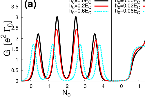
Figure 1: $G$=$dI/dV$ vs. $N_{0}$ in linear response for several values of $h_{0}$: (a) $T$=0.1$E_{C}$ and (b) $T$=0.

We now address the physics behind Fig. 1 — we investigate the SC states which arise in the IR, as well as how they evolved from the UV FP. To this end, we examine the QD’s spectral function (SF), $A_{d}(\omega)$. Fig. 2 shows $A_{d}(\omega)$ (at $T$=0) obtained via the LDECA. For comparison, results for $A_{d}(\omega)$ at the UV FP — obtained by formally setting {$t_{i}$}=0 — are shown in the insets. Fig. 2a shows $A_{d}(\omega)$ at the $N_{0}$=1/2 CB peak. Here we see a broad peak near $\omega$=0 i.e. near $E_{F}$; its features do not change much with $h_{0}$. From the insets, we see there was a redistribution of spectral weight, with much of the peak’s weight in the IR having been transferred from higher energies.

Figs. 2b and 2c show $A_{d}(\omega)$ in the CB valleys. A key feature is the narrow resonance which appears at or near $E_{F}$ — the Kondo resonance (KR). This resonance is a consequence of the SC state formed between the QD and leads due to the KE; its width represents the dynamically generated scale characteristic of the SC state — the Kondo temperature, $T_{K}$. As discussed below, the position and width of the KR are characteristic of the particular Kondo fixed point (KFP).

Fig. 2b shows $A_{d}(\omega)$ in the $N_{0}$=1 valley i.e. the 1/4-filled QD. For $h_{0}$=0, $A_{d}(\omega)$ exhibits a KR near $E_{F}$; for $h_{0}$$\neq$0, the resonance moves toward $E_{F}$ and its width narrows. As mentioned above, when $h_{0}$=0 the system has an SU(4) symmetry; $h_{0}$$\neq$0 reduces this symmetry to SU(2). For the 1/4-filled QD, the system flows to the SU(4) KFP when $h_{0}$=0, while $h_{0}$$\neq$0 drives the system to the SU(2) KFP; the KR is near (at) $E_{F}$ at the SU(4) (SU(2)) KFP with $T_{K}^{\rm SU(2)}$$<$$T_{K}^{\rm SU(4)}$. The UV and IR behaviors of $A_{d}(\omega)$ are compared in the insets — the KR is indeed an IR property, with its spectral weight taken from the higher energy UV peaks; interestingly, $h_{0}$ does not change the qualitative features of $A_{d}(\omega)$ at either the UV or IR FPs.

Fig. 2c shows $A_{d}(\omega)$ for $N_{0}$=2 i.e. the 1/2-filled QD — its behavior is drastically different from the SFs arising for both $N_{0}$=1/2 and $N_{0}$=1. For $h_{0}$=0, $A_{d}(\omega)$ exhibits a narrow KR at $E_{F}$; for $h_{0}$$\neq$0, the resonance splits and is suppressed. Hence, contrary to the 1/4-filled QD where $h_{0}$ drives the system from the SU(4) KFP to the SU(2) KFP, $h_{0}$ destroys the KE for the 1/2-filled QD. The UV and IR behaviors of $A_{d}(\omega)$ are compared in the insets — we see the KR suppressed as $h_{0}$ increases; as this occurs, the peaks at $\omega$=$\pm$$E_{C}$/2 regain spectral weight.

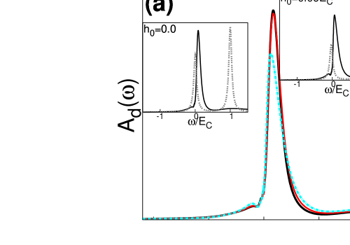
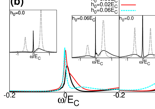
Figure 2: QD’s spectral function $A_{d}(\omega)$. (a) $A_{d}(\omega)$ for $N_{0}$=1/2. (b) $A_{d}(\omega)$ for $N_{0}$=1. (c) $A_{d}(\omega)$ for $N_{0}$=2. Insets: Comparison of $A_{d}(\omega)$ at the UV (gray dotted lines) and IR (solid black lines) fixed points.

Having discussed the QD’s SF in the various regimes, we now discuss (further) consequences of the SF’s features in the CB valleys i.e. for $N_{0}$$\simeq$$N$. To facilitate the analysis, we integrate out charge fluctuations on the QD; we arrive at the Coqblin-Schrieffer Hamiltoniankondobook

$$H_{\rm QD}=-\frac{J}{4}\left(\psi^{\dagger}_{\kappa s\phantom{{}^{\prime}}}f^{\phantom{\dagger}}_{\kappa s}\right)\left(f^{\dagger}_{\kappa^{\prime}s^{\prime}}\psi^{\phantom{\dagger}}_{\kappa^{\prime}s^{\prime}}\right)-\frac{h_{0}}{2}~{}f^{\dagger}_{\kappa s}\sigma^{z}_{\kappa\kappa^{\prime}}f^{\phantom{\dagger}}_{\kappa^{\prime}s}$$ (3)

where $\psi^{\phantom{\dagger}}_{\kappa s}$=$[t_{1}\psi^{\phantom{\dagger}}_{1\kappa s}(0)+t_{2}\psi^{\phantom{\dagger}}_{2\kappa s}(0)]$/$t$ with $t$=$\sqrt{t_{1}^{2}+t_{2}^{2}}$, $J=(4t^{2}/E_{C})\left[(N-N_{0}-1/2)^{-1}-(N-N_{0}+1/2)^{-1}\right]$, and the fermion operators satisfy the constraint $f^{\dagger}_{\kappa s}f^{\phantom{\dagger}}_{\kappa s}$=$N$ with $N$ being the number of particles on the QD. (While discussing the physics of the CB valleys, we write the QD’s fermion operators as $\{f_{\kappa s}\}$; also, Einstein summation convention is utilized). To treat Eq. 3, we consider a path integral representation of the partition function – we enforce the constraint $f^{\dagger}_{\kappa s}f^{\phantom{\dagger}}_{\kappa s}$=$N$ with a Lagrange multiplier field $\lambda$; we decouple the Kondo interaction using a Hubbard-Stratonovich field $\chi$.kondobook We arrive at an effective Hamiltonian

$$H_{\rm eff}=-\frac{h_{0}}{2}~{}f^{\dagger}_{\kappa s}\sigma^{z}_{\kappa\kappa^{\prime}}f^{\phantom{\dagger}}_{\kappa^{\prime}s}+\lambda\left(f^{\dagger}_{\kappa s}f^{\phantom{\dagger}}_{\kappa s}-N\right)$$ (4)

$$\ \ \ \ \ \ +\ \frac{4}{J}|\chi|^{2}+\chi^{\dagger}f^{\dagger}_{\kappa s}\psi^{\phantom{\dagger}}_{\kappa s}+\chi~{}\psi^{\dagger}_{\kappa s}f^{\phantom{\dagger}}_{\kappa s}\ .$$

Figure 3: $\chi$ field propagator ${\cal J}(i\omega_{m})$ — the solid (dashed) line denotes the leads’ ($f$-fermions’) Green’s function.

We begin by considering the physics at higher energies, focussing on the flow from the UV to the IR FPs. To do so, we treat the Bose fields $\chi$ and $\lambda$ in Eq. 4 in mean-field theory (MFT). Treating $\lambda$ in MFT amounts to treating the constraint $f^{\dagger}_{\kappa s}f^{\phantom{\dagger}}_{\kappa s}$=$N$ on average: $\langle f^{\dagger}_{\kappa s}f^{\phantom{\dagger}}_{\kappa s}\rangle$=$N$. To describe the physics near the UV FP, we take $\langle\chi\rangle$=0; the physics of the KE is contained in the effective action for $\chi$, obtained by integrating out the $f$-fermions and leads. To one-loop order, the propagator of the $\chi$ field ${\cal J}(i\omega_{m})$ is given by the diagram in Fig. 3 (with $\omega_{m}$ being a boson Matsubara frequency). Physically, ${\cal J}(i\omega_{m})$ is the running Kondo coupling.coleman

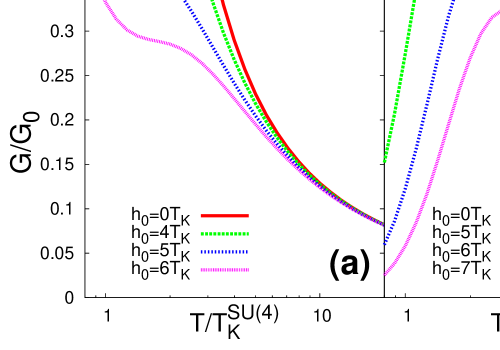
Figure 4: $G$/$G_{0}$ vs. $T$/$T_{K}^{\rm SU(4)}$ in linear response in the CB valleys: (a) 1/4-filled QD and (b) 1/2-filled QD.

Using our result for ${\cal J}(i\omega_{m})$, the current $I$=$\langle\hat{I}\rangle$ was computed as per Ref. landauer, ; results for $G$/$G_{0}$ vs. $T$/$T_{K}^{\rm SU(4)}$ are shown in Fig. 4, where

$$T_{K}^{\rm SU(4)}=D\exp\left(-1/\rho_{0}J\right)$$ (5)

with $D$ being half the leads’ bandwidth. [As before, $G_{0}$=($e^{2}$/$\pi$)4$\Gamma_{1}$$\Gamma_{2}$/($\Gamma_{1}$+$\Gamma_{2}$)².] Fig. 4a shows results for the 1/4-filled QD. To begin with, we see that $G$ grows logarithmically as $T$ is reduced — this is a consequence of the logarithmic growth of the running Kondo coupling.kondobook Furthermore, $G$/$G_{0}$ always grows to ${\cal O}(1)$ i.e. the system always flows to strong coupling. This is because the 1/4-filled QD exhibits a KE, irrespective of the value of $h_{0}$. However, $G$ grows more slowly for larger $h_{0}$ — the system flows to the SU(4) (SU(2)) KFP for smaller (larger) $h_{0}$; the slower growth of $G$ for larger $h_{0}$ occurs because $T_{K}^{\rm SU(2)}$$<$$T_{K}^{\rm SU(4)}$. (See Fig. 2b.)

Fig. 4b shows $G$/$G_{0}$ vs. $T$/$T_{K}^{\rm SU(4)}$ for the 1/2-filled QD; the results are drastically different from the 1/4-filled QD. As discussed above, whereas $h_{0}$ drives the system from the SU(4) to the SU(2) KFP for the 1/4-filled QD, $h_{0}$ destroys the KE for the 1/2-filled QD (see Fig. 2c); $G$ even becomes non-monotonic. Such behavior has been observed in magnetic alloys, where the occurrence of a spin glass phase freezes spin-flip processes and, hence, suppresses the KE.spinglass Here, larger values of $h_{0}$ freeze both spin and orbital processes. More precisely, $h_{0}$ cuts off the growth of the running Kondo coupling — for the 1/2-filled QD ${\cal J}$($T$)$\equiv$${\cal J}$($i\omega_{m}$=0) is given by

$$\rho_{0}{\cal J}(T)=J\left\{\ln\left(\frac{2\pi T}{T_{K}^{\rm SU(4)}}\right)+{\rm Re}\left[\psi\left(\frac{1}{2}+i\frac{h_{0}}{4\pi T}\right)\right]\right\}^{-1},$$

where $\psi(z)$ is the digamma function;gradshteyn as $\psi(z)$$\simeq$$\ln(z)$ for $|z|$$\gg$1, the growth of ${\cal J}$($T$) is suppressed for $h_{0}$ sufficiently larger than $T_{K}^{\rm SU(4)}$.

Having discussed the flow (in the CB valleys) from the UV to the KFPs in the IR, we now discuss further the physics of the SC KFPs. As before, we treat the Bose fields in Eq. 4 in MFT. Now, however, to describe the physics of the SC KFPs, we take $\langle\chi\rangle$=$\chi_{0}$($\neq$0).kondobook Hence, $\lambda$ and $\chi_{0}$ are determined via $\langle f^{\dagger}_{\kappa s}f^{\phantom{\dagger}}_{\kappa s}\rangle$=$N$ and $\chi_{0}$+$2J\langle\psi^{\dagger}_{\kappa s}f^{\phantom{\dagger}}_{\kappa s}\rangle$=0. With $\langle\chi\rangle$$\neq$0, the $f$-fermions SF is

$$A^{f}_{i}(\omega)=\frac{2\Gamma}{(\omega-\varepsilon_{i})^{2}+\Gamma^{2}}\$$

($\varepsilon_{1/2}$=$\lambda$$\pm$$h_{0}/2$), where $\Gamma$=$T_{K}$ when $T$=0.kondobook

Fig. 5 shows $G$/$G_{0}$ vs. $h_{0}$/$T_{K}^{\rm SU(4)}$ (computed as per Ref. landauer, ) at $T$=0. For the 1/4-filled QD, $G$/$G_{0}$=1 regardless of the value of $h_{0}$. This occurs because there is always a KE, $\Gamma$$\neq$0 — for small $h_{0}$, one is in the SU(4) Kondo regime; for larger $h_{0}$, one crosses over to the SU(2) Kondo regime. For the 1/2-filled QD, on the other hand, we see that $G$ depends on the magnitude of $h_{0}$ — $G$/$G_{0}$=2 for $h_{0}$=0 and decreases as $h_{0}$ is increased. [Within MFT, $G$$\rightarrow$0 for $h_{0}$=2$T_{K}^{\rm SU(4)}$.] This is because the SU(4) KE is destroyed and, consequently, the KR in the QD’s SF is suppressed for $h_{0}$ sufficiently large. (See Fig. 2c.)

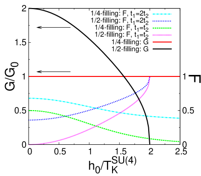
Figure 5: $G$/$G_{0}$ vs. $h_{0}$/$T_{K}^{\rm SU(4)}$ and $F$ vs. $h_{0}$/$T_{K}^{\rm SU(4)}$ in linear response at $T$=0.

Also shown in Fig. 5 are results for the noise (which has been shown to be a powerful probe of Kondo physicskondonoise ; kondonoiseexp ) at $T$=0. More specifically, we computed the zero-frequency noise

$$S(eV)=\int dt~{}\left[\langle\hat{I}(t)\hat{I}\rangle-\langle\hat{I}\rangle^{2}\right]$$ (6)

and, subsequently, the Fano factor $F$$\equiv$$S/2eI$ in linear response. While the conductance probes the spectral weight of the KR, the noise gives information about its position. Indeed, while both the SU(4) and SU(2) KEs give $G$/$G_{0}$=1 for the 1/4-filled QD, differences between the two can drastically be seen in $F$ — $F$ decreases as $h_{0}$ increases i.e. as we move from the SU(4) to the SU(2) KFP. This is seen most dramatically when $t_{1}$=$t_{2}$ where $F$$\rightarrow$0 as $h_{0}$ increases, but the qualitative behavior of $F$ is robust. [See the results for $t_{1}$=2$t_{2}$.] Physically, this arises because the KR in the QD’s SF is at $E_{F}$ at the SU(2) KFP, while it is away from $E_{F}$ at the SU(4) KFP. (See Fig. 2b.) For the 1/2-filled QD, $F$ increases as $h_{0}$ increases, approaching unity as $G$$\rightarrow$0; for $t_{1}$=$t_{2}$, $F$$\rightarrow$0 as $h_{0}$$\rightarrow$0. For $h_{0}$=0, the system is in a SC state, with a KR at $E_{F}$; as a result $F$=0 when $t_{1}$=$t_{2}$. As $h_{0}$ is increased, the SC state is destroyed and the system is driven to the weak-coupling regime; hence, $F$$\rightarrow$1 i.e. $F$ becomes Poissonian.noisereview

To summarize, we considered the behavior of CNT QDs in a magnetic field. We analyzed the evolution of the system from the UV to the IR FPs. We discussed the KEs that occur and their experimental consequences. In particular, the KEs arising for the 1/4-filled and 1/2-filled QDs were shown to be drastically different, with distinct signatures in the system’s transport; we are optimistic our results, particularly for the noise,noisecomment can be observed experimentally. Besides CNT QDs, our results are relevant to double QDs and, more generally, to QDs with two-fold orbital degeneracy.

This work was supported by the NSERC of Canada (MM and EHK), a SHARCNET Research Chair (MM and EHK), and the NSF (DMR - 0710529) (GBM).

References

- (1)
- (2) For reviews, see C. Dekker, Physics Today 52(5), 22 (1999); Physics World 13(6) (2000); R. Saito, G. Dresselhaus, and M. S. Dresselhaus, Physical Properties of Carbon Nanotubes (Imperial College Press, London 1998).
- (3) S. J. Tans, M. H. Deverot, H. Dai, A. Thess, R. E. Smalley, L. J. Geerligs, and C. Dekker, Nature (London) 386, 474 (1997); Z. Yao, H. W. Ch. Postma, L. Balents, and C. Dekker, Nature (London) 402, 273 (1999).
- (4) H. W. Ch. Postma, T. Teepen, Z. Yao, M. Grifoni, and C. Dekker, Science 293, 76 (2001).
- (5) C. Zhou, J. Kong, E. Yenilmez, and H. Dai, Science 290, 1552 (2000).
- (6) M. Bockrath, D. H. Cobden, P. L. McEuen, N. G. Chopra, A. Zettl, A. Thess, and R. E. Smalley, Science 275, 1922 (1997); J. Kong, C. Zhou, E. Yenilmez, and H. Dai, Appl. Phys. Lett. 77, 3977 (2000); M. J. Biercuk, S. Garaj, N. Mason, J. M. Chow, and C. M. Marcus, Nano Lett. 5, 1267 (2005).
- (7) J. Nygard, D. H. Cobden, and P. E. Lindelof, Nature 480, 342 (2000).
- (8) For a review, see, H. Grabert and M. H. Devoret, Eds., Single Charge Tunneling (Plenum, New York 1991).
- (9) L. Kouwenhoven and L. Glazman, Physics World 14(1), 33 (2001).
- (10) P. Jarillo-Herrero, J. Kong, H. S. J. van der Zant, C. Dekker, L. P. Kouwenhoven, and S. DeFranceschi, Nature 434, 484 (2005).
- (11) A. Makarovski, A. Zhukov, J. Liu, and G. Finkelstein, Phys. Rev. B 75, 241407(R) (2007).
- (12) A. Makarovski, J. Liu, and G. Finkelstein, Phys. Rev. Lett. 99, 066801 (2007).
- (13) M. S. Choi, R. Lopez, and R. Aguado, Phys. Rev. Lett. 95, 067204 (2005); J. S. Lim, M.-S. Choi, M. Y. Choi, R. Lopez, and R. Aguado, Phys. Rev. B 74, 205119 (2006).
- (14) E. Minot, Y. Yaish, V. Sazonova, and P. L. McEuen, Nature 428, 536 (2004).
- (15) F. B. Anders, D. E. Logan, M. R. Galpin, and G. Finkelstein, Phys. Rev. Lett. 100, 086809 (2008).
- (16) For a review of SU(4) KEs in nanostructures, see G. Zarand, Philos. Mag. 86, 2043 (2006).
- (17) Y. Meir and N. Wingreen, Phys. Rev. Lett. 68, 2512 (1992).
- (18) E. V. Anda, G. Chiappe, C. A. Büsser, M. A. Davidovich, G. B. Martins, F. Heidrich-Meisner, and E. Dagotto, Phys. Rev. B 70, 085308 (2008).
- (19) A. Hewson, The Kondo Effect to Heavy Fermions (Cambridge University Press, Cambridge 1993).
- (20) C. W. J. Beenakker, Phys. Rev. B 44, 1646 (1991).
- (21) P. Coleman, Phys. Rev. B 35, 5072 (1987).
- (22) See, e.g. F. Schopfer, C. Bäuerle, W. Rabaud, and L. Saminadayar, Phys. Rev. Lett. 90, 056801 (2003).
- (23) I. S. Gradshteyn and I. M. Ryzhik, Table of Integrals, Series, and Products (Academic Press, San Diego 1994).
- (24) Y. Meir and A. Golub, Phys. Rev. Lett. 88, 116802 (2002); E. Sela, Y. Oreg, F. von Oppen, and J. Koch, Phys. Rev. Lett. 97, 086601 (2006).
- (25) T. Delattre, C. Feuillet-Palma, L. G. Herrmann, P. Morfin, J.-M. Berroir, G. Feve, B. Placais, D. C. Glattli, M.-S. Choi, C. Mora, and T. Kontos, Nature Physics 5, 208 (2009).
- (26) Ya. M. Blanter and M. Büttiker, Phys. Rep. 336, 1 (2000).
- (27) Indeed, by working at lower temperatures and in a magnetic field, we are optimistic our results for the noise could be observed in the device/setup of Ref. kondonoiseexp, .