Improved Approximation Guarantees for Weighted Matching
in the Semi-Streaming Model

Abstract

We study the maximum weight matching problem in the semi-streaming model, and improve on the currently best one-pass algorithm due to Zelke (Proc. STACS ’08, pages 669–680) by devising a deterministic approach whose performance guarantee is $4.91+\varepsilon$. In addition, we study preemptive online algorithms, a sub-class of one-pass algorithms where we are only allowed to maintain a feasible matching in memory at any point in time. All known results prior to Zelke’s belong to this sub-class. We provide a lower bound of $4.967$ on the competitive ratio of any such deterministic algorithm, and hence show that future improvements will have to store in memory a set of edges which is not necessarily a feasible matching.

1 Introduction

The computational task of detecting maximum weight matchings is one of the most fundamental problems in discrete optimization, attracting plenty of attention from the operations research, computer science, and mathematics communities. (For a wealth of references on matching problems see [11].) In such settings, we are given an undirected graph $G=(V,E)$ whose edges are associated with non-negative weights specified by $w:E\to\mathbb{R}_{+}$. A set of edges $M\subseteq E$ is a matching if no two of the edges share a common vertex, that is, the degree of any vertex in $(V,M)$ is at most $1$. The weight $w(M)$ of a matching $M$ is defined as the combined weight of its edges, i.e., $\sum_{e\in M}w(e)$. The objective is to compute a matching of maximum weight. We study this problem in two related computational models: the semi-streaming model and the preemptive online model.

The semi-streaming model.

Even though these settings appear to be rather simple as first glance, it is worth noting that matching problems have an abundance of flavors, usually depending on how the input is specified. In this paper, we investigate weighted matchings in the semi-streaming model, was first suggested by Muthukrishnan [10]. Specifically, a graph stream is a sequence $e_{i_{1}},e_{i_{2}},\ldots$ of distinct edges, where $e_{i_{1}},e_{i_{2}},\ldots$ is an arbitrary permutation of $E$. When an algorithm is processing the stream, edges are revealed sequentially, one at a time. Letting $n=|V|$ and $m=|E|$, efficiency in this model is measured by the space $S(n,m)$ a graph algorithm uses, the time $T(n,m)$ it requires to process each edge, and the number of passes $P(n,m)$ it makes over the input stream. The main restriction is that the space $S(n,m)$ is limited to $O(n\cdot\mathrm{polylog}(n))$ bits of memory. We refer the reader to a number of recent papers [10, 3, 4, 2, 9] and to the references therein for a detailed literature review.

Online graph problems.

Unlike the semi-streaming model, in online problems the size of the underlying graph is not known in advance. The online matching problem has previously been modeled as follows. Edges are presented one by one to the algorithm, along with their weight. Once an edge is presented, we must make an irrevocable decision, whether to accept it or not. An edge may be accepted only if its addition to the set of previously accepted edges forms a feasible matching. In other words, an algorithm must keep a matching at all times, and its final output consists of all edges which were ever accepted. In this model, it is easy to verify that the competitive ratio of any (deterministic or randomized) algorithm exceeds any function of the number of vertices, meaning that no competitive algorithm exists. However, if all weights are equal, a greedy approach which accepts an edge whenever possible, has a competitive ratio of $2$, which is best possible for deterministic algorithms [7].

Similarly to other online settings (such as call control problems [5]), a preemptive model can be defined, allowing us to remove a previously accepted edge from the current matching at any point in time; this event is called preemption. Nevertheless, an edge which was either rejected or preempted cannot be inserted to the matching later on. We point out that other types of online matching problems were studied as well [7, 6, 8, 1].

Comparison between the models.

Both semi-streaming algorithms and online algorithms perform a single pass over the input. However, unlike semi-streaming algorithms, online algorithms are allowed to concurrently utilize memory for two different purposes. The first purpose is obviously to maintain the current solution, which must always be a feasible matching, implying that the memory size of this nature is bounded by the maximal size of a matching. The second purpose is to keep track of arbitrary information regarding the past, without any concrete bound on the size of memory used. Therefore, in theory, online algorithms are allowed to use much larger memory than is allowed in the semi-streaming model. Moreover, although this possibility is rarely used, online algorithms may perform exponential time computations whenever a new piece of input is revealed. On the other hand, a semi-streaming algorithm may re-insert an edge the current solution, even if it has been temporarily removed, as long as this edge was kept in memory. This extra power is not allowed for online (preemptive) algorithms, making them inferior in this sense in comparison to their semi-streaming counterparts.

Previous work.

Feigenbaum et al. [3] were the first to study matching problems under similar assumptions. Their main results in this context were a semi-streaming algorithm that computes a $(3/2-\varepsilon)$-approximation in $O(\log(1/\varepsilon)/\varepsilon)$ passes for maximum cardinality matching in bipartite graphs, as well as a one-pass $6$-approximation for maximum weighted matching in arbitrary graphs. Later on, McGregor [9] improved on these findings, to obtain performance guarantees of $(1+\varepsilon)$ and $(2+\varepsilon)$ for the maximum cardinality and maximum weight versions, respectively, being able to handle arbitrary graphs with only a constant number of passes (depending on $1/\varepsilon$). In addition, McGregor [9] tweaked the one-pass algorithm of Feigenbaum et al. into achieving a ratio of $5.828$. Finally, Zelke [12] has recently attained an improved approximation factor of $5.585$, which stands as the currently best one-pass algorithm. Note that the $6$-approximation algorithm in [3] and the $5.828$-approximation algorithm in [9] are preemptive online algorithms. On the other hand, the algorithm of Zelke [12] uses the notion of shadow-edges, which may be re-inserted into the matching, and hence it is not an online algorithm.

Main result I.

The first contribution of this paper is to improve on the above-mentioned results, by devising a deterministic one-pass algorithm in the semi-streaming model, whose performance guarantee is $4.91+\varepsilon$. In a nutshell, our approach is based on partitioning the edge set into $O(\log n)$ weight classes, and computing a separate maximal matching for each such class in online fashion, using $O(n\cdot\mathrm{polylog}(n))$ memory bits overall. The crux lies in proving that the union of these matchings contains a single matching whose weight compares favorably to the optimal one. The specifics of this algorithm are presented in Section 2.

Main result II.

Our second contribution is motivated by the relation between semi-streaming algorithms and preemptive online algorithms, which must maintain a feasible matching at any point in time. To our knowledge, there are currently no lower bounds on the competitive ratio that can be achieved by incorporating preemption. Thus, we also provide a lower bound of $4.967$ on the performance guarantee of any such deterministic algorithm. As a result, we show that improved one pass algorithms for this problem must store more than just a matching in memory. Further details are provided in Section 3.

2 The Semi-Streaming Algorithm

This section is devoted to obtaining main result I, that is, an improved one-pass algorithm for the weighted matching problem in the semi-streaming model. We begin by presenting a simple deterministic algorithm with a performance guarantee of $8$. We then show how to randomize its parameters, still within the semi-streaming framework, and obtain an expected approximation ratio of $4.9108$. Finally, we de-randomize the algorithm by showing how to emulate the required randomness using multiple copies (constant number) of the deterministic algorithm, while paying an additional additive factor of at most $\varepsilon$, for any fixed $\varepsilon>0$.

2.1 A simple deterministic approach

Preliminaries.

We maintain the maximum weight of any edge $w_{\max}$ seen so far in the input stream. Clearly, the maximum weight matching of the edges seen so far has weight in the interval $[w_{\max},{\frac{n}{2}w_{\max}}]$. Note that if we disregard all edges with weight at most $2\varepsilon w_{\max}\over n$, the weight of the maximum weight matching in the resulting instance decreases by an additive term of at most $\varepsilon w_{\max}\leq\varepsilon\mbox{{opt}}$.

Our algorithm has a parameter $\gamma>1$, and a value $\phi>0$. We define weight classes of edges in the following way. For every $i\in{\mathbb{Z}}$, we let the class $W_{i}$ be the collection of edges whose weight is in the interval $[\phi\gamma^{i},\phi\gamma^{i+1})$. We note that by our initial assumption, the weight of each edge is in the interval $[{2\varepsilon w_{\max}\over n},w_{\max}]$, and we say that a weight class $W_{i}$ is under consideration if its weight interval $[\phi\gamma^{i},\phi\gamma^{i+1})$ intersects $[{2\varepsilon w_{\max}\over n},w_{\max}]$. The number of classes which are under consideration at any point in time is $O(\log_{\gamma}(\frac{n}{\varepsilon}))$.

The algorithm.

Our algorithm simply maintains the list of classes under consideration and maintains a maximal (unweighted) matching for each such class. In other words, when the value of $w_{\max}$ changes, we delete from the memory some of these matchings, corresponding to the classes which stop being under consideration. Note that to maintain a maximal matching in a given subgraph, we only need to check if the two endpoints of the new edge are not covered by existing edges of the matching.

To conclude, for every new edge $e\in E$ we proceed as follows. We first check if $w(e)$ is greater than the current value of $w_{\max}$. If so, we update $w_{\max}$ and the list of weight classes under consideration accordingly. Then, we find the weight class of $w(e)$, and try to extend its corresponding matching, i.e., $e$ will be added to this matching if it remains a matching after doing so.

Note that at each point the content of the memory is the value $w_{\max}$ and a collection of $O(\log_{\gamma}(\frac{n}{\varepsilon}))$ matchings, consisting of $O(n\log_{\gamma}(\frac{n}{\varepsilon}))$ edges overall. Therefore, our algorithm indeed falls in the semi-streaming model.

At the conclusion of the input sequence, we need to return a single matching rather than a collection of matchings. To this end, we could compute a maximum weighted matching of the edges in the current memory. However, for the specific purposes of our analysis, we use the following faster algorithm. We sort the edges in memory in decreasing order of weight classes, such that the edges in $W_{i}$ appear before those in $W_{i-1}$, for every $i$. Using this sorted list of edges, we apply a greedy algorithm for selecting a maximal matching, in which the current edge is added to this matching if it remains a matching after doing so. Then, the post-processing time needed is linear in the size of the memory used, that is, $O(n\log_{\gamma}(\frac{n}{\varepsilon}))$. This concludes the presentation of the algorithm and its implementation as a semi-streaming algorithm.

Analysis.

For purposes of analysis, we round down the weight of each edge $e$ such that $w(e)\in W_{i}$ to be $\phi\gamma^{i}$. This way, we obtain rounded edge weights. Now fix an optimal solution opt and denote by opt its weight, and by $\mbox{{opt}}^{\prime}$ its rounded weight. The next claim immediately follows from the definition of $W_{i}$.

Lemma 2.1.

$\mbox{{opt}}\leq\gamma\mbox{{opt}}^{\prime}$.

As an intermediate step, we analyze an improved algorithm which keeps all weight classes. That is, for each $i$, we use $M_{i}$ to denote the maximal matching of class $W_{i}$ at the end of the input, and denote by $M$ the solution obtained by this algorithm, if we would have applied it. Similarly, we denote by $\mbox{{opt}}_{i}$ the set of edges in opt which belong to $W_{i}$. For every $i$, we define the set of vertices $P_{i}$, associated with $W_{i}$, to be the set of endpoints of edges in $M_{i}$ that are not associated with higher weight classes:

$$P_{i}=\{\,u,v\ |\ (u,v)\in M_{i}\}\setminus(P_{i+1}\cup P_{i+2}\cup\cdots).$$

For a vertex $p\in P_{i}$, we define its associated weight to be $\phi\gamma^{i}$. For vertices which do not belong to any $P_{i}$, we let their associated weight be zero. We next bound the total associated weight of all the vertices.

Lemma 2.2.

The total associated weight of all the vertices is at most ${2\gamma\over\gamma-1}\cdot w(M)$.

• Consider a vertex $u\in P_{i}$ and let $(u,v)$ be the edge in $M_{i}$ adjacent to $u$. If $(u,v)\in M$ then we charge the weight associated with $u$ to the edge $(u,v)$. Thus, an edge $e\in M_{i}$ is charged at most twice from vertices associated with its own weight class. Otherwise, if $(u,v)\notin M$ then there must be some other edge $e\in M\cap M_{j}$, for some $j>i$, that prevented us from adding $(u,v)$ to $M$, in which case we charge the weight associated with $u$ to $e$. Notice that $u\notin e$, for otherwise, $u$ would not be associated with $W_{i}$. Thus, the edge $e\in M_{j}$ must be of the form $e=(v,x)$ and can only be charged twice from vertices in weight class $i$, once through $v$ and once through $x$.

To bound the ratio between $w(M)$ and the total associated weight of the vertices, it suffices to bound the ratio between the weight of an edge $e\in M$ and the total associated weight of the vertices which are charged to $e$. Assume that $e\in M_{j}$, then there are at most two vertices which are charged to $e$ and class $i$ for all $i\leq j$, and no vertex is associated to $e$ and class $i$ for $i>j$. Hence, the total associated weight of these vertices is at most

$$2\sum_{i\leq j}\phi\gamma^{i}<2\phi\gamma^{j}\cdot\sum_{i^{\prime}=0}^{\infty}{1\over\gamma^{i^{\prime}}}=2\phi\gamma^{j}\cdot{1\over{1-1/\gamma}}=\phi\gamma^{j}\cdot{2\gamma\over\gamma-1},$$

and the claim follows since $w(e)\geq\phi\gamma^{j}$.  

It remains to bound $\mbox{{opt}}^{\prime}$ with respect to the total associated weight.

Lemma 2.3.

$\mbox{{opt}}^{\prime}$ is at most the total weight associated with all vertices.

• It suffices to show that for every edge $e=(x,y)\in\mbox{{opt}}_{i}$ the maximum of the associated weights of $x$ and $y$ is at least the rounded weight of $e$. Suppose that this claim does not hold, then $x$ and $y$ are not covered by $M_{i}$, as otherwise their associated weight would be at least $\phi\gamma^{i}$. Hence, when the algorithm considered $e$, we would have added $e$ to $M_{i}$, contradicting our assumption that $x$ and $y$ are not covered by $M_{i}$.  

Using the above sequence of lemmas, and recalling that we lose another $\varepsilon$ in the approximation ratio due to disregarding edges of weight at most $2\varepsilon w_{\max}\over n$, we obtain the following inequality:

$$\mbox{{opt}}\leq\gamma\mbox{{opt}}^{\prime}\leq\left(\gamma\cdot{2\gamma\over\gamma-1}+\varepsilon\right)\cdot w(M).$$ (2.1)

Therefore, we establish the following theorem.

Theorem 2.4.

Our simple deterministic algorithm has an approximation ratio of $({2\gamma^{2}\over\gamma-1}+\varepsilon)$. This ratio can be optimized to $8+\varepsilon$ by picking $\gamma=2$.

The next example demonstrates that the analysis leading to Theorem 2.4 is tight.

Example 2.5.

Let $k$ be some large enough integer and $\varepsilon>0$ be sufficiently small. Consider the instance depicted in Figure 1, where $M=M_{k}$ consists of a single edge $(x,y)$ with weight $\gamma^{k}$. For every $0\leq i<k$, the matching $M_{i}$ consists of exactly two edges $(\alpha_{i},x)$ and $(y,\beta_{i})$ each of weight $\gamma^{i}$, and $\mbox{{opt}}_{i}$ consists of two edges $(\alpha_{i},a_{i})$ and $(\beta_{i},b_{i})$ each of weight $\gamma^{i+1}-\varepsilon$. In addition, there are two edges $(a_{k},x)$ and $(b_{k},y)$ whose weight is $\gamma^{k+1}-\varepsilon$. It is easy to see that each $M_{i}$ is indeed maximal in its own weight class. Given these matchings, our greedy selection rule will output a single edge $(x,y)$ with total weight $\gamma^{k}$ (notice that computing a maximum weight matching in $M_{0}\cup\cdots\cup M_{k}$ does not help when $\gamma\geq 2$). Moreover, the value of the optimal solution matches our upper bound up to an additive $O(\varepsilon)$ term.

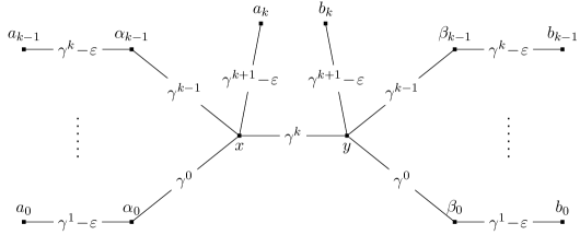
Figure 1: A tight example for our deterministic algorithm.

2.2 Improved approximation ratio through randomization

In what follows, we analyze a randomized variant of the deterministic algorithm which was presented in the previous subsection. In general, this variant sets the value of $\phi$ to be $\phi=\gamma^{\delta}$ where $\delta$ is a random variable. This method is commonly referred to as randomized geometric grouping.

Formally, let $\delta$ be a continuous random variable which is uniformly distributed on the interval $[0,1)$. We define the weight class $W_{i}(\delta)=[\gamma^{i+\delta},\gamma^{i+1+\delta})$, and run the algorithm as in the previous subsection. Note that this algorithm uses only the partition of the edges into classes and not the precise values of their weights. In addition, we denote by $M(\delta)$ the resulting matching obtained by the algorithm, and by $TW(\delta)$ the total associated weight of the vertices, where for a vertex $p\in P_{i}$ we define its associated weight to be $\gamma^{i+\delta}$ (i.e., the minimal value in the interval $W_{i}(\delta)$). We also denote by $\mbox{{opt}}^{\prime}(\delta)$ the value of $\mbox{{opt}}^{\prime}$ for this particular $\delta$.

For any fixed value of $\delta$, inequality (2.1) immediately implies $\mbox{{opt}}^{\prime}(\delta)\leq({2\gamma\over\gamma-1}+\varepsilon)\cdot w(M(\delta)).$ Note that $\mbox{{opt}}^{\prime}(\delta)$ and $w(M(\delta))$ are random variables, such that for each realization of $\delta$ the above inequality holds. Hence, this inequality holds also for their expected values. That is, we have established the following lemma where $\mathrm{E}_{\delta}[\cdot]$ represents expectation with respect to the random variable $\delta$.

Lemma 2.6.

$\mathrm{E}_{\delta}[\mbox{{opt}}^{\prime}(\delta)]\leq({2\gamma\over\gamma-1}+\varepsilon)\cdot\mathrm{E}_{\delta}[w(M(\delta))]$.

We next lower bound opt in terms of $\mathrm{E}_{\delta}[\mbox{{opt}}^{\prime}(\delta)]$.

Lemma 2.7.

$\frac{\gamma\ln\gamma}{\gamma-1}\cdot\mathrm{E}_{\delta}[\mbox{{opt}}^{\prime}(\delta)]\geq\mbox{{opt}}$.

• We will show the corresponding inequality for each edge $e\in\mbox{{opt}}$. We denote by $w^{\prime}_{\delta}(e)$ the rounded weight of $e$ for a specific value of $\delta$. Then, it suffices to show that $\frac{\gamma\ln\gamma}{\gamma-1}\cdot\mathrm{E}_{\delta}[w^{\prime}_{\delta}(e)]\geq w(e)$. Let $p$ be an integer, and let $0\leq\alpha<1$ be the value that satisfies $w(e)=\gamma^{p+\alpha}$. Then, for $\delta\leq\alpha$, $w^{\prime}_{\delta}(e)=\gamma^{p+\delta}$, and for $\delta>\alpha$, $w^{\prime}_{\delta}(e)=\gamma^{p-1+\delta}$, thus the expected rounded weight of $e$ over the choices of $\delta$ is

  $$\mathrm{E}_{\delta}[w^{\prime}_{\delta}(e)]=\int_{0}^{\alpha}\gamma^{p+\delta}d\delta+\int_{\alpha}^{1}\gamma^{p-1+\delta}d\delta={1\over\ln\gamma}\cdot\left(\gamma^{p}(\gamma^{\alpha}-1)+\gamma^{p-1}(\gamma-\gamma^{\alpha})\right)=w(e)\cdot\left(1-\frac{1}{\gamma}\right){1\over\ln\gamma},$$

  and the claim follows.  

Combining the above two lemmas we obtain that the expected weight of the resulting solution is at least $(\frac{(\gamma-1)^{2}}{2\gamma^{2}\ln\gamma}+\varepsilon)\cdot\mbox{{opt}}$. This approximation ratio is optimized for $\gamma\approx 3.513$, where it is roughly $(4.9108+\varepsilon)$. Hence, we have established the following theorem.

Theorem 2.8.

The randomized algorithm has an approximation ratio of roughly $4.9108+\varepsilon$.

2.3 Derandomization

Prior to presenting our de-randomization, we slightly modify the randomized algorithm of the previous subsection. In this variation, instead of picking $\delta$ uniformly at random from the interval $[0,1)$ we pick $\delta^{\prime}$ uniformly at random from the discrete set $\{0,{1\over q},{2\over q},\ldots,{q-1\over q}\}$. We apply the same method as in the previous section where we replace $\delta$ by $\delta^{\prime}$. Then, using Lemma 2.6, we obtain $\mathrm{E}_{\delta^{\prime}}[\mbox{{opt}}^{\prime}(\delta^{\prime})]\leq({2\gamma\over\gamma-1}+\varepsilon)\cdot\mathrm{E}_{\delta^{\prime}}[w(M(\delta^{\prime}))]$. To extend Lemma 2.7 to this new setting, we note that $\delta^{\prime}$ can be obtained by first picking $\delta$ and then rounding it down to the largest number in $\{0,{1\over q},{2\over q},\ldots,{q-1\over q}\}$ which is at most $\delta$. In this way, we couple the distributions of $\delta$ and $\delta^{\prime}$. Now consider the rounded weight of an edge $e$ in opt in the two distinct values of $\delta$ and $\delta^{\prime}$. The ratio between the two rounded weight is at most $\gamma^{1/q}$. Therefore, we establish that $\frac{\gamma\ln\gamma}{\gamma-1}\cdot\gamma^{1/q}\cdot\mathrm{E}_{\delta}[\mbox{{opt}}^{\prime}(\delta)]\geq\mbox{{opt}}$. Therefore, the resulting approximation ratio of the new variation is $\frac{2\gamma^{2+1/q}\ln\gamma}{(\gamma-1)^{2}}+\varepsilon$. By settinf $q$ to be large enough (picking $q=\lceil\frac{1}{\log_{\gamma}(\varepsilon/5)}\rceil$ is enough), the resulting approximation ratio is bounded by $\frac{2\gamma^{2}\ln\gamma}{(\gamma-1)^{2}}+2\varepsilon$.

De-randomizing the new variation in the semi-streaming model is straightforward. We simply run in parallel all $q$ possible outcomes of the algorithm, one for each possible value of $\delta^{\prime}$, and pick the best solution among the $q$ solutions we obtained. Since $q$ is a constant (for fixed values of $\varepsilon$), the resulting algorithm is still a semi-streaming algorithm whose performance guarantee is $4.9108+2\varepsilon$. By scaling $\varepsilon$ prior to applying the algorithm, we establish the following result.

Theorem 2.9.

For any fixed $\varepsilon>0$, there is a deterministic one-pass semi-streaming $(4.9108+\varepsilon)$-approximation algorithm for the weighted matching problem. This algorithm processes each input edge in constant time and required $O(n)$ time at the end of the input to compute the final output.

3 Online Preemptive Matching

In this section, we established the following theorem.

Theorem 3.1.

The competitive ratio of any deterministic preemptive online algorithm is at least ${\cal{R}}\approx 4.967$, where ${\cal{R}}$ is the unique real solution of the equation $x^{3}=4(x^{2}+x+1)$.

Recall that the algorithms of [3] and [9] can be viewed as online preemptive algorithms; their competitive ratios are $6$ and $5.828$, respectively.

Definitions of some constants.

Let ${\cal{C}}={\cal{R}}-\varepsilon$ for some $\varepsilon>0$ and assume that a deterministic online algorithm achieves a competitive ratio of at most ${\cal{C}}^{\prime}={\cal{C}}-\varepsilon$. We construct an input graph iteratively, and show that after a finite number of steps, the competitive ratio is violated.

In the construction of the input, all edge weights come from two weight sequences. The main weight sequence is $w_{1},w_{2},\ldots$, and an additional weight function is $w^{\prime}_{2},w^{\prime}_{3},\ldots$. These sequences are defined as follows:

• $w_{1}=1$, and $w_{k+1}=\frac{1}{2{\cal{C}}+1}(({\cal{C}}^{2}+1)w_{k}-{\cal{C}}\sum_{i=1}^{k-1}w_{i})$ for $k\geq 1$.

• $w^{\prime}_{k+1}=\frac{1}{{\cal{C}}}(({\cal{C}}+1)w_{k+1}-w_{k})$.

The first sequence is defined for $k+1$ only as long as $w_{k-1}\geq w_{k-2}$. As soon as $w_{k}<w_{k-1}$, the sequence stops with $w_{k+1}$, and the length of the sequence $w_{i}$ is $n=k+1$. We later show that such a value $k$ must exist. Let $S_{i}=\sum_{j=1}^{i}w_{j}$ (and $S_{0}=0$).

Properties of the sequences.

By definition, since $w^{\prime}_{i+1}=w_{i+1}+\frac{1}{{\cal{C}}}(w_{i+1}-w_{i})$, if $w_{k}<w_{k-1}$, then $w_{k+1}<w_{k}$ holds as well. Note that $w_{i}\leq w^{\prime}_{i}$ for all $i<n-1$, by definition, since $w_{i}\geq w_{i-1}$, but $w^{\prime}_{n-1}<w_{n-1}$. In addition, we have the following:

$$w^{\prime}_{i+1}+w_{i+1}+S_{i-1}={\cal{C}}w_{i}.$$

This equality holds for $i=1,2,\ldots,n-2$ since

$$w^{\prime}_{i+1}+w_{i+1}+S_{i-1} = {{\cal{C}}+1\over{\cal{C}}}w_{i+1}-{w_{i}\over{\cal{C}}}+w_{i+1}+S_{i-1}$$

$$= {2{\cal{C}}+1\over{\cal{C}}}\cdot{1\over 2{\cal{C}}+1}\cdot(({\cal{C}}^{2}+1)w_{i}-{\cal{C}}S_{i-1})+S_{i-1}-{w_{i}\over{\cal{C}}}$$

$$= {\cal{C}}w_{i},$$

where the first equality holds by definition of $w^{\prime}_{i+1}$, the second equality holds by definition of $w_{i+1}$, and the third one by simple algebra. In addition,

$$S_{i-2}+w_{i}+w_{i+1}+w^{\prime}_{i+1}={\cal{C}}w^{\prime}_{i}.$$

The last equality holds for $i=2,3,\ldots,n-2$ since

$$S_{i-2}+w_{i}+w_{i+1}+w^{\prime}_{i+1} = S_{i-2}+w_{i}+{2{\cal{C}}+1\over{\cal{C}}}w_{i+1}-{w_{i}\over{\cal{C}}}$$

$$= S_{i-2}+{{\cal{C}}-1\over{\cal{C}}}w_{i}+{2{\cal{C}}+1\over{\cal{C}}}\cdot\frac{1}{2{\cal{C}}+1}(({\cal{C}}^{2}+1)w_{i}-{\cal{C}}S_{i-1}))$$

$$= ({\cal{C}}+1)w_{i}+S_{i-2}-S_{i-1}$$

$$= ({\cal{C}}+1)w_{i}-w_{i-1}$$

$$= {\cal{C}}w^{\prime}_{i},$$

where the first equality holds by definition of $w^{\prime}_{i+1}$, the second by definition of $w_{i+1}$, the third by simple algebra, the fourth by definition of $S_{i-1}$ and $S_{i-2}$, and the last one by definition of $w^{\prime}_{i}$.

Input construction, step 1.

To better understand our construction, we advice the reader to consult Figure 2. The input is created in $n$ steps. In the initial step, two edges $(a_{1},x_{1})$ and $(b_{1},x_{1})$, each of weight $w_{1}$, are introduced. Assume that after both edges have arrived, the online algorithm holds the edge $(a_{1},x_{1})$. All future edges either have endpoints which are new vertices, or in the set $\{a_{1},x_{1}\}$ (i.e., they do not contain $b_{1}$ as an endpoint). An optimal solution keeps $(b_{1},x_{1})$.

Figure 2: An example of five steps of the lower bound construction. The curved edges denote the edge kept by the online algorithm at each time. In the first two steps, the edges $(x_{i},a_{i})$ are chosen by the algorithm. In the third step $(x_{3},a_{3})$ is not chosen by the algorithm, so $(y_{3},c_{3})$ arrives next. In the fourth $(x_{4},a_{4})$ is not chosen by the algorithm, so $(y_{4},c_{4})$ arrives next. In the fifth step $(x_{5},a_{5})$ is chosen by the algorithm, so no further edges arrive in this step.

Input construction, properties.

Every future step can be of two distinct types, which will be described later on. Among the edges introduced below, vertices called $b_{j}$ denote endpoints which occur each on a single edge.

After step $i$, the following invariants are maintained. The algorithm keeps a single edge denoted by $e_{i}$. If $i=1$, then $e_{i}=(a_{i},x_{i})$. If $i>1$, then this edge can be one of two edges, $(a_{i},x_{i})$ or $(c_{i},y_{i})$. If $e_{i}=(a_{i},x_{i})$, then its weight is $w_{i}$, and an optimal solution has one edge of each weight $w_{1},w_{2},\ldots,w_{i-1},w_{i}$. No future edges will have common endpoints with these $i$ edges, except, possibly, with the endpoint $x_{i}$ of the edge of weight $w_{i}$ (the edge of this weight which this optimal solution keeps is always $(x_{i},b_{i})$). Otherwise, $e_{i}=(c_{i},y_{i})$, and its weight is $w^{\prime}_{i}$, in which case an optimal solution can have edges of weights $w_{1},w_{2},\ldots,w_{i}$, except for one weight $w_{j}$ for some $j<i$. This index $j$ is used in the definition of the next step, and the properties of the current step. In addition to these $i-1$ edges, the optimal solution also has the edge $(c_{i},y_{i})$. Future edges will have endpoints which are new vertices, or in the set $\{c_{i},y_{i}\}$. In the last case, the vertex $y_{i}$ is equal to the vertex $x_{j}$. The invariants clearly hold after the first step. We next define all other steps and show that the invariants hold for each option.

Input construction, step $\boldsymbol{n}$.

If $i+1=n$, the last step consists of an edge of weight $w_{n}$. Let $x_{n}=a_{n-1}$, if $e_{n-1}=(a_{n-1},x_{n-1})$ and otherwise $x_{n}=c_{n-1}$. The new edge is $(x_{n},b_{n})$, where $b_{n}$ is a new vertex. This edge has a common endpoint with the edge that the algorithm has. In fact, the algorithm has an edge of weight at least $w_{n-1}>w_{n}$, and thus we assume that it does not preempt it. If the algorithm has an edge of weight $w_{n-1}$, the edge $(x_{n},b_{n})$ does not have $x_{i}$ as an endpoint, so adding the new edge to the optimal solution does not require the removal of any edges, and the profit of the optimal solution is $S_{n}$. If the algorithm has an edge of weight $w^{\prime}_{n-1}$, the new edge is $(c_{n-1},b_{n})$. We replace the edge $(c_{n-1},y_{n-1})$ of the optimal solution by the new edge. In addition, the edge $(y_{n-1},b_{j})=(x_{j},b_{j})$ (where $j$ is the index such that the optimal solution before the modification of the current step does not have an edge of weight $w_{j}$) is added to the optimal solution, since the endpoint $y_{n-1}$ became free, and the endpoint $b_{j}$ only has degree 1. The profit of the optimal solution is $S_{n}$ again. Recall that $w^{\prime}_{n-1}\leq w_{n-1}$, and hence the algorithm earns (in both cases) at most $w_{n-1}$. Note also that the optimal solution has value of $S_{n}$ and if $w_{n}<0$ then we can drop the edge of this weight from the optimal solution and get a solution of value $S_{n-1}$. Therefore, we will use $S_{n-1}$ as a lower bound on the value of the optimal solution in this case. Thus we will show later that $\frac{S_{n-1}}{w_{n-1}}\geq{\cal{C}}>{\cal{C}}^{\prime}$.

Input construction, step $\boldsymbol{i+1}$, for $\boldsymbol{i+1<n}$.

We next show how to construct the edges of step $i+1$, for the case $i+1<n$. We introduce two new edges of weight $w_{i+1}$. Let $x_{i+1}=a_{i}$, if $e_{i}=(a_{i},x_{i})$ and otherwise $x_{i+1}=c_{i}$. The new edges are $(x_{i+1},b_{i+1})$, and $(x_{i+1},a_{i+1})$, where $a_{i+1}$ and $b_{i+1}$ are new vertices. Both these edges have a common endpoint with the edge that the algorithm has, and the algorithm can either preempt the edge it has, in which case we assume (without loss of generality) that it now has $(x_{i+1},a_{i+1})$, or else it keeps the previous edge. If the algorithm keeps the previous edge, let $y_{i+1}=x_{i}$, if $e_{i}=(a_{i},x_{i})$ and otherwise $y_{i+1}=y_{i}$. In this case a third edge, $(y_{i+1},c_{i+1})$, which has a weight of $w^{\prime}_{i+1}$, is introduced. The vertex $c_{i+1}$ is new.

There are four cases to consider. In the first case, if the algorithm replaces the edge $(a_{i},x_{i})$ with the edge $(x_{i+1},a_{i+1})=(a_{i},a_{i+1})$, then an optimal solution can add the edge $(x_{i+1},b_{i+1})$ to its edges, since the endpoint $b_{i+1}$ is new, and the endpoint $a_{i}$ was introduced in the previous step, in which the optimal solution obtained the edge $(x_{i},b_{i})$.

If the algorithm replaces the edge $(c_{i},y_{i})$ with the edge $(x_{i+1},a_{i+1})=(c_{i},a_{i+1})$, an optimal solution can remove the edge $(c_{i},y_{i})$ from its solution and add the two edges $(x_{i+1},b_{i+1})=(c_{i},b_{i+1})$ and $(y_{i},b_{j})=(x_{j},b_{j})$ (where $j$ is the index such that the optimal solution before the modification of the current step does not have an edge of weight $w_{j}$). This is possible since the endpoints $b_{i+1}$ and $b_{j}$ do not have other edges, and the endpoints $c_{i}$ and $y_{i}$ become free.

In the last two cases, the invariants hold. For the remaining two cases note that if $w^{\prime}_{i}\leq 0$ or $w_{i}<0$ and the algorithm has a single edge of weight $w^{\prime}_{i}$ or $w_{i}$, respectively, then the optimal solution is strictly positive and the value of the algorithm is non-positive, and hence the resulting approximation ratio in this case is unbounded. Hence, we can assume without loss of generality that if the algorithm has a single edge at the end of step $i$, then its weight is strictly positive.

If the algorithm does not replace the edge $(a_{i},x_{i})$ with the edge $(x_{i+1},a_{i+1})=(a_{i},a_{i+1})$, we show that it must replace it with the edge $(y_{i+1},c_{i+1})=(x_{i},c_{i+1})$. Assume that this is not the case. Then the profit of the algorithm is $w_{i}$ and the optimal solution can omit its edge $(x_{i},b_{i})$ and add the edges $(x_{i},c_{i+1})$ and $(a_{i},b_{i+1})$ (since all these endpoints are introduced in steps $i$ and $i+1$, except for $x_{i}$, which becomes free). Thus the profit of the optimal algorithm is $S_{i-1}+w_{i+1}+w^{\prime}_{i+1}={\cal{C}}\cdot w_{i}$, while the profit of the online algorithm is $w_{i}$. Thus, the algorithm must switch to the edge $(x_{i+1},a_{i+1})$, and the structure of the optimal solution is according to the invariants.

If the algorithm does not replace the edge $(c_{i},y_{i})$ with the edge $(x_{i+1},a_{i+1})=(c_{i},a_{i+1})$, we show that it must replace it with the edge $(y_{i+1},c_{i+1})=(y_{i},c_{i+1})$. Assume that this is not the case. Then the profit of the algorithm is $w^{\prime}_{i}$ and the optimal solution can omit its edge $(c_{i},y_{i})$ and add the edges $(c_{i},a_{i+1})$ and $(y_{i},c_{i+1})$ (since $c_{i}$ and $y_{i}$ become free, and the other two endpoints are introduced in step $i+1$). Thus the profit of the optimal algorithm is $S_{i}-w_{j}+w_{i+1}+w^{\prime}_{i+1}$, where $j\leq i-1$ and $i\geq 2$, since $w_{j}\leq w_{j+1}\leq\cdots\leq w_{i-1}$ as $i-1\leq n-2$, we get that the optimal profit is at least $S_{i-2}+w_{i}+w_{i+1}+w^{\prime}_{i+1}={\cal{C}}w^{\prime}_{i}$, while the profit of the online algorithm is $w^{\prime}_{i}$. Thus, the algorithm must switch to the edge $(x_{i+1},a_{i+1})$, and the structure of the optimal solution is according to the invariants.

Bounding the competitive ratio.

We next define a recursive formula for $S_{i}$. By the definition of the sequence $w_{i}$, we have

$$\left\{\begin{array}[]{l}S_{0}=0\\ S_{1}=1\\ S_{k+1}=\frac{{\cal{C}}^{2}+2{\cal{C}}+2}{2{\cal{C}}+1}S_{k}-\frac{{\cal{C}}^{2}+{\cal{C}}+1}{2{\cal{C}}+1}S_{k-1},\quad\mbox{for }k\geq 1\end{array}\right.$$ (3.1)

We first use this recurrence to show that if $w_{n-1}<w_{n-2}$ then ${S_{n-1}\over w_{n-1}}\geq{\cal{C}}$. To see this note that by assumption $S_{n-1}-S_{n-2}<S_{n-2}-S_{n-3}$, hence using the recurrence formula we conclude that

$$S_{n-1}-2S_{n-2}+{2{\cal{C}}+1\over-{\cal{C}}^{2}-{\cal{C}}-1}S_{n-1}+{{\cal{C}}^{2}+2{\cal{C}}+2\over{\cal{C}}^{2}+{\cal{C}}+1}S_{n-2}<0,$$

that is,

$$S_{n-1}\cdot({\cal{C}}^{2}+{\cal{C}}+1-2{\cal{C}}-1)+S_{n-2}\cdot({\cal{C}}^{2}+2{\cal{C}}+2-2{\cal{C}}^{2}-2{\cal{C}}-2)<0,$$

which is equivalent to $({\cal{C}}^{2}-{\cal{C}})S_{n-1}-{\cal{C}}^{2}S_{n-2}<0$, so ${\cal{C}}(S_{n-1}-S_{n-2})<S_{n-1}$, and we conclude that ${\cal{C}}w_{n-1}<S_{n-1}$, as we argued. Therefore, it remains to show that there is a value of $n$ such that $w_{n-2}>w_{n-1}$. To establish this claim, it suffices to show that there is a value of $j$ for which $w_{j}<0$ (since $w_{1}>0$). To prove this last claim, we will show that there is a value of $k$ such that $S_{k}<0$. Finally, to show the existence of such $k$, we will solve the linear homogeneous recurrence formula, and use the explicit form of $S_{k}$ to show that there is a value of $k$ such that $S_{k}<0$.

To solve the recurrence formula (3.1), we guess solutions of the form $S_{k}=x^{k}$ for all $k$, and get the following quadratic equation for $x$:

$$(2{\cal{C}}+1)x^{2}-({\cal{C}}^{2}+2{\cal{C}}+2)x+({\cal{C}}^{2}+{\cal{C}}+1)=0.$$

We solve this quadratic equation and get its solutions

$$x_{1,2} = {({\cal{C}}^{2}+2{\cal{C}}+2)\pm\sqrt{({\cal{C}}^{2}+2{\cal{C}}+2)^{2}-4(2{\cal{C}}+1)({\cal{C}}^{2}+{\cal{C}}+1)}\over 2(2{\cal{C}}+1)}$$

$$= {({\cal{C}}^{2}+2{\cal{C}}+2)\pm\sqrt{{\cal{C}}^{4}+4{\cal{C}}^{2}+4+4{\cal{C}}^{3}+8{\cal{C}}+4{\cal{C}}^{2}-8{\cal{C}}^{3}-4{\cal{C}}^{2}-8{\cal{C}}^{2}-4{\cal{C}}-8{\cal{C}}-4}\over 2(2{\cal{C}}+1)}$$

$$= {({\cal{C}}^{2}+2{\cal{C}}+2)\pm\sqrt{{\cal{C}}({\cal{C}}^{3}-4{\cal{C}}^{2}-4{\cal{C}}-4)}\over 2(2{\cal{C}}+1)}.$$

Note that using ${\cal{C}}<{\cal{R}}$, and recalling that ${\cal{R}}$ is the unique real solution of the equation $x^{3}=4(x^{2}+x+1)$, we conclude that ${\cal{C}}({\cal{C}}^{3}-4{\cal{C}}^{2}-4{\cal{C}}-4)<0$ and hence the two solutions are complex numbers whose imaginary parts are not zero. Since we got two distinct solutions of $x$, it is known that the recurrence formula (3.1) is solved by a formula of the form $S_{i}=\alpha x_{1}^{i}+\beta x_{2}^{i}$ where $\alpha$ and $\beta$ are constants. We find the value of $\alpha$ and $\beta$ using the conditions $S_{0}=0$ and $S_{1}=1$. So we get the following set of two equations: $\alpha+\beta=0$ (corresponding to $S_{0}=0$), and $\alpha x_{1}+\beta x_{2}=1$ (corresponding to $S_{1}=1$). From the first equation we conclude that $\beta=-\alpha$, and using this we obtain $\alpha={1\over x_{1}-x_{2}}={2{\cal{C}}+1\over\sqrt{{\cal{C}}({\cal{C}}^{3}-4{\cal{C}}^{2}-4{\cal{C}}-4)}}$. Hence, the closed form solution of $S_{j}$ for values of ${\cal{C}}<{\cal{R}}$ is as follows.

$$S_{j} = {2{\cal{C}}+1\over\sqrt{{\cal{C}}({\cal{C}}^{3}-4{\cal{C}}^{2}-4{\cal{C}}-4)}}\left({({\cal{C}}^{2}+2{\cal{C}}+2)+\sqrt{{\cal{C}}({\cal{C}}^{3}-4{\cal{C}}^{2}-4{\cal{C}}-4)}\over 2(2{\cal{C}}+1)}\right)^{j}$$ (3.2)

$$-{2{\cal{C}}+1\over\sqrt{{\cal{C}}({\cal{C}}^{3}-4{\cal{C}}^{2}-4{\cal{C}}-4)}}\left({({\cal{C}}^{2}+2{\cal{C}}+2)-\sqrt{{\cal{C}}({\cal{C}}^{3}-4{\cal{C}}^{2}-4{\cal{C}}-4)}\over 2(2{\cal{C}}+1)}\right)^{j}\ .$$

We use the notation $i=\sqrt{-1}$, and let $\alpha=A\cdot i$. As noted above ${\cal{C}}({\cal{C}}^{3}-4{\cal{C}}^{2}-4{\cal{C}}-4)<0$, and hence $A$ is a real number. We also define $r$ and $\theta$ such that ${({\cal{C}}^{2}+2{\cal{C}}+2)+\sqrt{{\cal{C}}({\cal{C}}^{3}-4{\cal{C}}^{2}-4{\cal{C}}-4)}\over 2(2{\cal{C}}+1)}=r(\cos(\theta)+i\sin(\theta))$, and also ${({\cal{C}}^{2}+2{\cal{C}}+2)-\sqrt{{\cal{C}}({\cal{C}}^{3}-4{\cal{C}}^{2}-4{\cal{C}}-4)}\over 2(2{\cal{C}}+1)}=r(\cos(\theta)-i\sin(\theta))$, then we get the following formula for $S_{j}$.

$$S_{j} = A\cdot i\cdot\left(r^{j}(\cos(\theta)+i\sin(\theta))^{j}-r^{j}(\cos(\theta)-i\sin(\theta))^{j}\right)$$

$$= A\cdot i\cdot\left(r^{j}(\cos(j\theta)+i\sin(j\theta))-r^{j}(\cos(j\theta)-i\sin(j\theta))\right)$$

$$= A\cdot i\cdot r^{j}\cdot 2i\sin(j\theta)$$

$$= -2Ar^{j}\sin(j\theta)\ .$$

Note that $r^{j}>0$ for all $j$, and hence to show that the sequence $\{S_{j}\}$ changes its sign as we required, it suffices to show that the sequence $\{\sin(j\theta)\}$ changes its sign, but this last claim holds because $0<\theta<\pi$ (as the solutions $x_{1}$ and $x_{2}$ are not real numbers). Hence, the claim follows.

References

- [1] N. Bansal, N. Buchbinder, A. Gupta, and J. Naor. An -competitive algorithm for metric bipartite matching. In Proceedings of the 15th Annual European Symposium on Algorithms, pages 522–533, 2007.
- [2] M. Elkin and J. Zhang. Efficient algorithms for constructing -spanners in the distributed and streaming models. Distributed Computing, 18(5):375–385, 2006.
- [3] J. Feigenbaum, S. Kannan, A. McGregor, S. Suri, and J. Zhang. On graph problems in a semi-streaming model. Theoretical Computer Science, 348(2-3):207–216, 2005.
- [4] J. Feigenbaum, S. Kannan, A. McGregor, S. Suri, and J. Zhang. Graph distances in the data-stream model. SIAM Journal on Computing, 38(5):1709–1727, 2008.
- [5] J. A. Garay, I. S. Gopal, S. Kutten, Y. Mansour, and M. Yung. Efficient on-line call control algorithms. Journal of Algorithms, 23(1):180–194, 1997.
- [6] B. Kalyanasundaram and K. Pruhs. Online weighted matching. Journal of Algorithms, 14(3):478–488, 1993.
- [7] R. M. Karp, U. V. Vazirani, and V. V. Vazirani. An optimal algorithm for on-line bipartite matching. In Proceedings of the 22nd Annual ACM Symposium on Theory of Computing, pages 352–358, 1990.
- [8] S. Khuller, S. G. Mitchell, and V. V. Vazirani. On-line algorithms for weighted bipartite matching and stable marriages. Theoretical Computer Science, 127(2):255–267, 1994.
- [9] A. McGregor. Finding graph matchings in data streams. In Proceedings of the 8th International Workshop on Approximation Algorithms for Combinatorial Optimization Problems, pages 170–181, 2005.
- [10] S. Muthukrishnan. Data Streams: Algorithms and Applications. Foundations and Trends in Theoretical Computer Science. Now Publishers Inc, 2005.
- [11] A. Schrijver. Combinatorial Optimization: Polyhedra and Efficiency. Springer, 2003.
- [12] M. Zelke. Weighted matching in the semi-streaming model. In Proceedings of the 25th Annual Symposium on Theoretical Aspects of Computer Science, pages 669–680, 2008.