Adiabatic versus Isocurvature Non–Gaussianity

Abstract

We study the extent to which one can distinguish primordial non–Gaussianity (NG) arising from adiabatic and isocurvature perturbations. We make a joint analysis of different NG models based on various inflationary scenarios: local-type and equilateral-type NG from adiabatic perturbations and local-type and quadratic-type NG from isocurvature perturbations together with a foreground contamination by point sources. We separate the Fisher information of the bispectrum of CMB temperature and polarization maps by $l$ for the skew spectrum estimator introduced by Munshi & Heavens (2009) to study the scale dependence of the signal-to-noise ratio of different NG components and their correlations. We find that the adiabatic and the isocurvature modes are strongly correlated, though the phase difference of acoustic oscillations helps to distinguish them. The correlation between local- and equilateral-type is weak, but the two isocurvature modes are too strongly correlated to be discriminated. Point source contamination, to the extent to which it can be regarded as white noise, can be almost completely separated from the primordial components for $l>100$. Including correlations among the different components, we find that the errors of the NG parameters increase by 20-30% for the WMAP 5-year observation, but $\simeq 5\%$ for Planck observations.

1 Introduction

The statistical properties of fluctuations in the early Universe can be used to probe the very earliest stages of its history, and provide valuable information on the mechanisms which ultimately gave rise to the existence of structure within it. This may include evidence for the cosmic inflationary expansion. With the recent claim of a detection of non–Gaussianity (Yadav & Wandelt, 2008) in the Wilkinson Microwave Anisotropy Probe (WMAP) sky maps, interest in primordial non–Gaussianity has obtained a tremendous boost.

Non-Gaussianity from the simplest inflationary models based on a single slowly-rolling scalar field is typically very small (Salopek & Bond, 1990; Falk et al., 1993; Gangui et al., 1994; Acquaviva et al., 2003; Maldacena, 2003; Bartolo, Matarrese & Riotto, 2006). Variants of the simple inflationary models can lead to much higher levels of non–Gaussianity, such as multiple fields (Linde & Mukhanov, 1997; Lyth, Ungarelli & Wands, 2003); modulated reheating scenarios (Dvali, Gruzinov & Zaldarriaga, 2004); warm inflation (Gupta et al., 2002; Moss & Xiong, 2007); ekpyrotic model (Koyama et al., 2007).

Different forms are proposed to describe primordial non–Gaussianity. Much interest has focused on local-type $f_{\rm NL}$ by which the non–Gaussianity of Bardeen’s curvature perturbations is locally characterized (Gangui et al., 1994; Verde et al., 2000; Wang & Kamionkowski, 2000; Komatsu & Spergel, 2001; Babich & Zaldarriaga, 2004):

$$\Phi(x)=\phi(x)+f_{\rm NL}(\phi^{2}(x)-\langle\phi^{2}(x)\rangle),$$ (1)

where $\phi$ is the linear Gaussian part of $\Phi$. This form is motivated by the single-field inflation scenarios and then many models predict non–Gaussianity in terms of $f_{\rm NL}$ (Bartolo et al., 2004). Optimized estimators of the bispectrum, which is the leading correlation term in the local form, are introduced by Heavens (1998) and have been successively developed to the point where an estimator for $f_{\rm NL}$ saturates the Cramér-Rao bound for partial sky coverage and inhomogeneous noise (Komatsu, Spergel & Wandelt, 2005; Creminelli et al., 2006; Creminelli, Senatore, & Zaldarriaga, 2007; Medeiros & Contaldi, 2006; Cabella et al., 2006; Liguori et al., 2007; Komatsu et al., 2009; Smith, Senatore & Zaldarriaga, 2009).

The local-type $f_{\rm NL}$ is sensitive to the bispectrum with squeezed-configuration triangles ($k_{1}\ll k_{2}\sim k_{3}$). Several models including the inflation scenario with non-canonical kinetic terms (Seery & Lidsey, 2005; Chen, Easther & Lim, 2007), Dirac-Born-Infeld models (Alishahiha, Silverstein & Tong, 2004), and Ghost inflation (Arkani-Hamed et al., 2004) predict large NG signals in equilateral configuration triangles ($\ell_{1}\simeq\ell_{2}\simeq\ell_{3}$), which is well described with equilateral-type $f_{\rm NL}$ (Babich, Creminelli & Zaldarriaga, 2004).

Non-Gaussianity arising from primordial isocurvature (entropy) perturbations has been discussed in the context of NG field potentials (Linde & Mukhanov, 1997; Peebles, 1999; Boubekeur & Lyth, 2006; Suyama & Takahashi, 2008), the curvaton scenario (Lyth, Ungarelli & Wands, 2003; Bartolo et al., 2004; Beltran, 2008; Moroi & Takahashi, 2009), modulated reheating (Boubekeur & Creminelli, 2006), baryon asymmetry (Kawasaki, Nakayama & Takahashi, 2009), and the axion (Kawasaki et al., 2008). Hikage et al. (2009) first put observational limits on the isocurvature non-Gaussianity using WMAP 5-year data.

In this paper, we make a joint analysis of the different NG models to estimate the extent to which one can decode each NG information from CMB temperature (T) and E polarization (E) maps obtained by WMAP and Planck. We separate Fisher information of the CMB bispectrum by different ranges of $l$ to study at which angular scale each NG parameter has large S/N and correlations among different NG components weaken. This idea is based on a new estimator called skew spectrum, which Munshi & Heavens (2009) has introduced to measure a scale dependence of NG parameters, while the commonly-used single skewness parameter (Komatsu, Spergel & Wandelt, 2005) gives a single value averaged over all scales. The advantage of the new estimator is that it retains information on the source of the non-Gaussianity, which the commonly-used one does not.

For our analysis, we adopt a set of cosmological parameters at the maximum likelihood values for a power-law $\Lambda$CDM model from the WMAP 5-year data only fit (Dunkley et al., 2009): $\Omega_{\rm b}=0.0432$; $\Omega_{\rm cdm}=0.206$; $\Omega_{\Lambda}=0.7508$; $H_{0}=72.4~{}{\rm km~{}s^{-1}~{}Mpc^{-1}}$; $\tau=0.089$; $n_{\phi}=0.961$. The amplitude of the primordial power spectrum is set to be $2.41\times 10^{-9}$ at $k=0.002{\rm Mpc}^{-1}$. The spectra of isocurvature perturbations are assumed to be scale-invariant. The radiation transfer functions for adiabatic and isocurvature perturbations are computed using the publicly-available CMBFAST code (Seljak & Zaldarriaga, 1996).

This paper is organized as follows: different NG models from primordial adiabatic and isocurvature perturbations are introduced in §2; §3 presents a Fisher matrix analysis of these parameters in which we estimate the corresponding error expected from WMAP and Planck observations; §4 devotes to a summary.

2 Models of Primordial Non-Gaussianity

We consider various forms to describe primordial non–Gaussianity from adiabatic and isocurvature perturbations, and then provide explicit expressions for the bispectra.

2.1 Local-Type Adiabatic component

The bispectrum in the local-type NG form (eq.[1]) is written as (e.g., Komatsu & Spergel, 2001)

$$B^{\rm Adi,Loc}(k_{1},k_{2},k_{3})=2f_{\rm NL}^{\rm Adi,Loc}[P_{\phi}(k_{1})P_{\phi}(k_{2})~{}~{}~{}~{}~{}~{}~{}~{}~{}~{}~{}~{}~{}$$

$$+P_{\phi}(k_{2})P_{\phi}(k_{3})+P_{\phi}(k_{3})P_{\phi}(k_{1})],$$ (2)

where we rewrite $f_{\rm NL}$ in the equation (1) as $f_{\rm NL}^{\rm Adi,Loc}$. The CMB angular bispectra for $T$, $E$, and their cross terms are given by

$$b_{XYZ,l_{1}l_{2}l_{3}}^{\rm Adi,Loc}=2f_{\rm NL}^{\rm Adi,Loc}\int r^{2}dr[\beta_{Xl_{1}}^{\rm Adi}(r)\beta_{Yl_{2}}^{\rm Adi}(r)\alpha_{Zl_{3}}^{\rm Adi}(r)$$

$$+\beta_{Xl_{1}}^{\rm Adi}(r)\alpha_{Yl_{2}}^{\rm Adi}(r)\beta_{Zl_{3}}^{\rm Adi}(r)+\alpha_{Xl_{1}}^{\rm Adi}(r)\beta_{Yl_{2}}^{\rm Adi}(r)\beta_{Zl_{3}}^{\rm Adi}(r)]$$ (3)

where $X,Y$, and $Z$ denote $T$ or $E$, and $\alpha_{Xl}^{\rm Adi}$ and $\beta_{Xl}^{\rm Adi}$ are defined with the adiabatic radiation transfer function $g_{Xl}^{\rm Adi}$ as

$$\alpha_{Xl}^{\rm Adi}(r) \equiv \frac{2}{\pi}\int k^{2}dkg_{Xl}^{\rm Adi}(k)j_{l}(kr),$$ (4)

$$\beta_{Xl}^{\rm Adi}(r) \equiv \frac{2}{\pi}\int k^{2}dkP_{\phi}(k)g_{Xl}^{\rm Adi}(k)j_{l}(kr).$$ (5)

2.2 Equilateral-Type Adiabatic Component

The bispectrum in the equilateral-type NG form is characterized by the NG parameter $f_{\rm NL}^{\rm Adi,Eq}$ (Babich, Creminelli & Zaldarriaga, 2004) as follows:

$$B^{\rm Adi,Eq}(k_{1},k_{2},k_{3})=6f_{\rm NL}^{\rm Adi,Eq}[-P_{\phi}(k_{1})P_{\phi}(k_{2})-P_{\phi}(k_{2})P_{\phi}(k_{3})$$

$$-P_{\phi}(k_{3})P_{\phi}(k_{1})-2\{P_{\phi}(k_{1})P_{\phi}(k_{2})P_{\phi}(k_{3})\}^{2/3}$$

$$+\{[P_{\phi}(k_{1})P_{\phi}(k_{2})^{2}P_{\phi}(k_{3})^{3}]^{1/3}+(5~{}{\rm perm.})\}].$$

The CMB angular bispectra in this form are given by

$$b_{XYZ,l_{1}l_{2}l_{3}}^{\rm Adi,Eq}=6f_{\rm NL}^{\rm Adi,Eq}\int r^{2}dr[-\beta_{Xl_{1}}^{\rm Adi}(r)\beta_{Yl_{2}}^{\rm Adi}(r)\alpha_{Zl_{3}}^{\rm Adi}(r)$$

$$-\beta_{Xl_{1}}^{\rm Adi}(r)\alpha_{Yl_{2}}^{\rm Adi}(r)\beta_{Zl_{3}}^{\rm Adi}(r)-\alpha_{Xl_{1}}^{\rm Adi}(r)\beta_{Yl_{2}}^{\rm Adi}(r)\beta_{Zl_{3}}^{\rm Adi}(r)$$

$$-2\delta_{Xl_{1}}^{\rm Adi}(r)\delta_{Yl_{2}}^{\rm Adi}(r)\delta_{Zl_{3}}^{\rm Adi}(r)$$

$$+\{\beta_{Xl_{1}}^{\rm Adi}(r)\gamma_{Yl_{2}}^{\rm Adi}(r)\delta_{Zl_{3}}^{\rm Adi}(r)+(5{\rm perm.})\}],$$ (7)

where

$$\gamma_{Xl}^{\rm Adi}(r) \equiv \frac{2}{\pi}\int k^{2}dkP_{\phi}^{1/3}(k)g_{Xl}^{\rm Adi}(k)j_{l}(kr),$$ (8)

$$\delta_{Xl}^{\rm Adi}(r) \equiv \frac{2}{\pi}\int k^{2}dkP_{\phi}^{2/3}(k)g_{Xl}^{\rm Adi}(k)j_{l}(kr).$$ (9)

2.3 Isocurvature Components

Here we consider an isocurvature perturbation ${\cal S}$ between axion-type cold dark matter (CDM) and radiation, which is uncorrelated with adiabatic perturbations, defined as

$${\cal S}\equiv\frac{\delta\rho_{\rm CDM}}{\rho_{\rm CDM}}-\frac{3\delta\rho_{\gamma}}{4\rho_{\gamma}},$$ (10)

where $\rho_{\rm CDM}$ is the CDM energy density and $\rho_{\gamma}$ is the radiation energy density. The fractional isocurvature perturbation $f_{\rm S}$ is defined as

$$f_{\rm S}\equiv\frac{P_{\cal S}(k_{0})}{P_{\zeta}(k_{0})+P_{\cal S}(k_{0})}.$$ (11)

where $P_{\zeta}$ and $P_{\cal S}$ represent the power spectra of $\zeta$ and ${\cal S}$ and $k_{0}$ is set to be 0.002Mpc^-1. At linear order, $\Phi$ (eq.[1]) is related to $\zeta$ by $\Phi=(3/5)\zeta$. The definition of $f_{\cal S}$ is same as the commonly used parameter $\alpha$ (Bean et al., 2006). The current observational limit on $f_{\rm S}$ is 0.067 (95% CL) for the axion-type isocurvature perturbation (Komatsu et al., 2009).

2.3.1 Local-Type Isocurvature Component

We consider two different forms for isocurvature non-Gaussianity. One is the same local form as the adiabatic one (eq.[2.1]):

$$B^{\rm Iso,Loc}(k_{1},k_{2},k_{3})=2f_{\rm NL}^{\rm Iso,Loc}[P_{\eta}(k_{1})P_{\eta}(k_{2})~{}~{}~{}~{}~{}~{}~{}~{}~{}~{}~{}~{}~{}~{}$$

$$+P_{\eta}(k_{2})P_{\eta}(k_{3})+P_{\eta}(k_{3})P_{\eta}(k_{1})],$$ (12)

where $\eta$ denotes the Gaussian part of ${\cal S}$ with the amplitude of $P_{\eta}(k)$ is normalized by $f_{\rm S}$ (eq.[11]). The parameter $f_{\rm NL}^{\rm Iso,Loc}$ corresponds to $\alpha^{2}f_{\rm NL}^{\rm ISO}$ in Hikage et al. (2009). We obtain the CMB bispectrum as

$$b_{XYZ,l_{1}l_{2}l_{3}}^{\rm Iso,Loc}=2f_{\rm NL}^{\rm Iso,Loc}\int r^{2}dr[\beta_{Xl_{1}}^{\rm Iso}(r)\beta_{Yl_{2}}^{\rm Iso}(r)\alpha_{Zl_{3}}^{\rm Iso}(r)$$

$$+\beta_{Xl_{1}}^{\rm Iso}(r)\alpha_{Yl_{2}}^{\rm Iso}(r)\beta_{Zl_{3}}^{\rm Iso}(r)+\alpha_{Xl_{1}}^{\rm Iso}(r)\beta_{Yl_{2}}^{\rm Iso}(r)\beta_{Zl_{3}}^{\rm Iso}(r)],$$ (13)

where $\alpha_{Xl}^{\rm Iso}$ and $\beta_{Xl}^{\rm Iso}$ are defined with the isocurvature radiation transfer function $g_{Xl}^{\rm Iso}$ as

$$\alpha_{Xl}^{\rm Iso}(r) \equiv \frac{2}{\pi}\int k^{2}dkg_{Xl}^{\rm Iso}(k)j_{l}(kr),$$ (14)

$$\beta_{Xl}^{\rm Iso}(r) \equiv \frac{2}{\pi}\int k^{2}dkP_{\eta}(k)g_{Xl}^{\rm Iso}(k)j_{l}(kr).$$ (15)

2.3.2 Quadratic-Type Isocurvature Component

When the linear Gaussian term is negligible compared with the quadratic term, the isocurvature perturbation has a $\chi^{2}$ from (e.g., Linde & Mukhanov, 1997):

$${\cal S}=\sigma^{2}-\langle\sigma^{2}\rangle,$$ (16)

where $\sigma$ obeys Gaussian statistics. This form has been studied in the context of axion (Kawasaki et al., 2008) and curvaton scenarios (Langlois, Vernizzi & Wands, 2008). The bispectra are calculated as (Komatsu, 2002)

$$B^{\rm Iso,Quad}(k_{1},k_{2},k_{3})=\frac{8}{3}\int_{L_{\rm box}^{-1}}\frac{d^{3}{\mathbf{p}}}{(2\pi)^{3}}P_{\sigma}(p)~{}~{}~{}~{}~{}~{}~{}~{}~{}~{}~{}~{}~{}~{}~{}~{}~{}~{}$$

$$\times[P_{\sigma}(|{\mathbf{k}_{1}}+{\mathbf{p}}|)P_{\sigma}(|{\mathbf{k}_{2}}-{\mathbf{p}}|)+P_{\sigma}(|{\mathbf{k}_{2}}+{\mathbf{p}}|)P_{\sigma}(|{\mathbf{k}_{3}}-{\mathbf{p}}|)$$

$$+P_{\sigma}(|{\mathbf{k}_{3}}+{\mathbf{p}}|)P_{\sigma}(|{\mathbf{k}_{1}}-{\mathbf{p}}|)],$$ (17)

where a finite box-size $L_{\rm box}$ gives an infrared cutoff. To avoid assumptions at scales far beyond the present horizon $H_{0}^{-1}$, we set $L_{\rm box}=30$Gpc. The equation (2.3.2) is approximately given by Hikage et al. (2009) as

$$b_{XYZ,l_{1}l_{2}l_{3}}^{\rm Iso,Quad}=2\int r^{2}dr[\beta_{Xl_{1}}^{\rm Iso,Quad}(r)\beta_{Yl_{2}}^{\rm Iso}(r)\alpha_{Zl_{3}}^{\rm Iso}(r)~{}~{}~{}~{}~{}~{}~{}~{}~{}~{}~{}~{}~{}$$

$$+\beta_{Xl_{1}}^{\rm Iso}(r)\alpha_{Yl_{2}}^{\rm Iso}(r)\beta_{Zl_{3}}^{\rm Iso,Quad}(r)+\alpha_{Xl_{1}}^{\rm Iso}(r)\beta_{Yl_{2}}^{\rm Iso,Quad}(r)\beta_{Zl_{3}}^{\rm Iso}(r)],$$

where

$$\beta_{Xl}^{\rm Iso,Quad}(r) \equiv \frac{2}{\pi}\int_{L_{\rm box}^{-1}}k^{2}dkP_{\cal S}(k)g_{Xl}^{\rm Iso}(k)j_{l}(kr),$$ (19)

$$\beta_{Xl}^{\rm Iso}(r) \equiv \frac{2}{\pi}\int_{L_{\rm box}^{-1}}k^{2}dkP_{\sigma}(k)g_{Xl}^{\rm Iso}(k)j_{l}(kr).$$ (20)

Non-Gaussianity in this form is characterized by $f_{\rm S}$ (eq.[11]).

2.4 Point Source Component

Unmasked point sources (e.g., radio galaxies) generates an additional non–Gaussianity in observed CMB maps. Assuming them to be Poisson distribution, $b_{XYZ,l_{1}l_{2}l_{3}}^{\rm PS}$ is a constant.

3 Fisher Information Analysis for Skew Spectrum

We make Fisher information analysis of the different NG components introduced in the previous section to estimate the error expected from WMAP, Planck and noiseless ideal observations.

The Fisher matrix for the CMB bispectrum in the weakly non-Gaussian, all-sky limit is written as (Babich & Zaldarriaga, 2004; Yadav, Komatsu,& Wandelt, 2007)

$$F^{ij} = \sum_{l}F_{l}^{ij},$$ (21)

$$F_{l}^{ij} = \sum_{2\leq l_{1}\leq l_{2}\leq l}I^{2}_{l_{1}l_{2}l}\sum_{XYZ}\sum_{PQR}$$ (22)

$$\times b_{XYZ,l_{1}l_{2}l}^{i}({\bf Cov}^{-1})_{l_{1}l_{2}l}^{XYZ|PQR}b_{PQR,l_{1}l_{2}l}^{j},$$

where $i$ and $j$ denote each NG component and the factor $I_{l_{1}l_{2}l_{3}}$ is defined as

$$I_{l_{1}l_{2}l_{3}}\equiv\sqrt{\frac{(2l_{1}+1)(2l_{2}+1)(2l_{3}+1)}{4\pi}}\left(\begin{array}[]{ccc}l_{1}&l_{2}&l_{3}\\ 0&0&0\end{array}\right).$$ (23)

The sums over $XYZ$ and $PQR$ are just $TTT$ when using CMB temperature maps only (T only), but are eight combinations ($TTT,TTE,TET,ETT,TEE,ETE,EET,EEE$) when both CMB temperature and E polarization maps are used (T&E). The Fisher matrix at each $l$, $F_{l}^{ij}$, is associated with the skew spectrum estimator for the $i$-th NG component, $S_{l}^{i}$, defined as (Munshi & Heavens, 2009)

$$S_{l}^{i} = \frac{1}{2l+1}\sum_{2\leq l_{1}\leq l_{2}\leq l}I^{2}_{l_{1}l_{2}l}\sum_{XYZ}\sum_{PQR}$$ (24)

$$\times b_{XYZ,l_{1}l_{2}l}^{i}({\bf Cov}^{-1})_{l_{1}l_{2}l}^{XYZ|PQR}b_{PQR,l_{1}l_{2}l}^{\rm obs},$$

where $b^{\rm obs}_{l_{1}l_{2}l}$ denotes the observed bispectrum. The relation to the single skewness estimator $S_{\rm prim}^{i}$ (Komatsu, Spergel & Wandelt, 2005) is

$$S_{\rm prim}^{i}=\sum_{l}(2l+1)S_{l}^{i}.$$ (25)

When non–Gaussianity is small, the covariance matrix is approximately given by

$${\bf Cov}_{l_{1}l_{2}l_{3}}^{XYZ|PQR}\simeq\Delta_{l_{1}l_{2}l_{3}}C_{l_{1}}^{XP}C_{l_{2}}^{YQ}C_{l_{3}}^{ZR},$$ (26)

where $\Delta_{l_{1}l_{2}l_{3}}$ is 6 ($l_{1}=l_{2}=l_{3}$), 2 ($l_{1}=l_{2}$, $l_{2}=l_{3}$, or $l_{1}=l_{3}$), and 1 ($l_{1}\neq l_{2}\neq l_{3}$) and $C_{l}^{XY}$ represents the CMB power spectrum from purely adiabatic perturbations including observational noise $N_{l}^{XY}$:

$$C_{l}^{XY}=\frac{2}{\pi}\int k^{2}dkP_{\phi}(k)g_{Xl}^{\rm Adi}(k)g_{Yl}^{\rm Adi}(k)+N_{l}^{XY}.$$ (27)

We consider three different noise/beam functions: an ideal case without noise/beam (“Ideal”); WMAP 5-year V+W band coadded map (“WMAP5”); Planck’s expectations after two full sky surveys for 14 months (“Planck”) using all of nine frequency channels. Noise is assumed to be homogeneous white noise and $N_{l}^{XY}=0$ when $X\neq Y$. Noise/beam is coadded at each $l$ with the inverse weight of the noise variance in each frequency band or differential assembly. Planck’s noise/beam information is obtained from http://www.rssd.esa.int/Planck). The fraction of sky $f_{\rm sky}$ is set to be 1 in this analysis.

Figure 1 shows the diagonal component of the Fisher matrix $F_{l}^{ii}$ (eq.[22]). It represents the square of signal-to-noise ratio $(S/N)^{2}$ for $i$-th NG component at $l$ without correlations among different NG components. The adiabatic components have an increasing trend of $S/N$ at higher $l$. The majority of the signal of the isocurvature components in temperature maps come from the large-angular scale ($l<100$), where isocurvature perturbations produce larger CMB fluctuations than adiabatic perturbations. A phase difference in acoustic oscillations between adiabatic and isocurvature modes provides a distinct signature seen around $l\sim 300$, which is important particularly when polarization maps are included. Table 1 lists the values of the diagonal components of the Fisher matrix summed over $l$ up to 2500, at which Planck estimates are enough saturated.

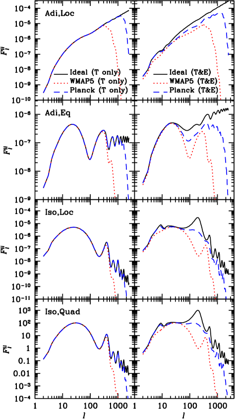
Figure 1: Diagonal components of the Fisher matrix $F_{l}^{ii}$ (eq.[22]). From top to bottom, the local-type adiabatic (Adi,Loc), the equilateral-type adiabatic (Adi,Eq), the local-type isocurvature (Iso,Loc), and the quadratic-type isocurvature (Iso,Quad) components are plotted. Left panels are for T map only, but right panels are for T&E maps. Noise/Beam is for Ideal (solid), WMAP5 (dotted) and Planck observations (dashed).

Table 1: Diagonal components of the Fisher matrix $F^{ii}$ summed up to $l=2500$. The different noise/beam for WMAP5, Planck, and Ideal are considered.

	Adi,Loc	Adi,Eq	Iso,Loc	Iso,Quad
WMAP5 (T only)	2.7$\times 10^{-3}$	7.2$\times 10^{-5}$	2.9$\times 10^{-4}$	6.8$\times 10^{3}$
Planck (T only)	3.7$\times 10^{-2}$	2.3$\times 10^{-4}$	3.1$\times 10^{-4}$	7.6$\times 10^{3}$
Ideal (T only)	9.0$\times 10^{-2}$	3.4$\times 10^{-4}$	3.1$\times 10^{-4}$	7.7$\times 10^{3}$
WMAP5 (T&E)	3.0$\times 10^{-3}$	7.5$\times 10^{-5}$	3.1$\times 10^{-4}$	7.2$\times 10^{3}$
Planck (T&E)	5.8$\times 10^{-2}$	4.8$\times 10^{-4}$	8.9$\times 10^{-4}$	2.6$\times 10^{4}$
Ideal (T&E)	3.6$\times 10^{-1}$	2.9$\times 10^{-3}$	3.9$\times 10^{-3}$	1.3$\times 10^{5}$

Figure 2 shows the cross-correlation coefficient $r_{l}$ defined as $r_{l}\equiv F_{l}^{ij}/(F_{l}^{ii}F_{l}^{jj})^{1/2}$. The local-type adiabatic and isocurvature components are strongly correlated, but the phase difference of acoustic oscillations weakens the correlation, as seen especially around $l\sim 200$. The correlation between the local-type and the equilateral-type components becomes weak at $l>100$. The two isocurvature components are almost completely correlated over all scales. The correlation with the point source component is very weak for $l>100$.

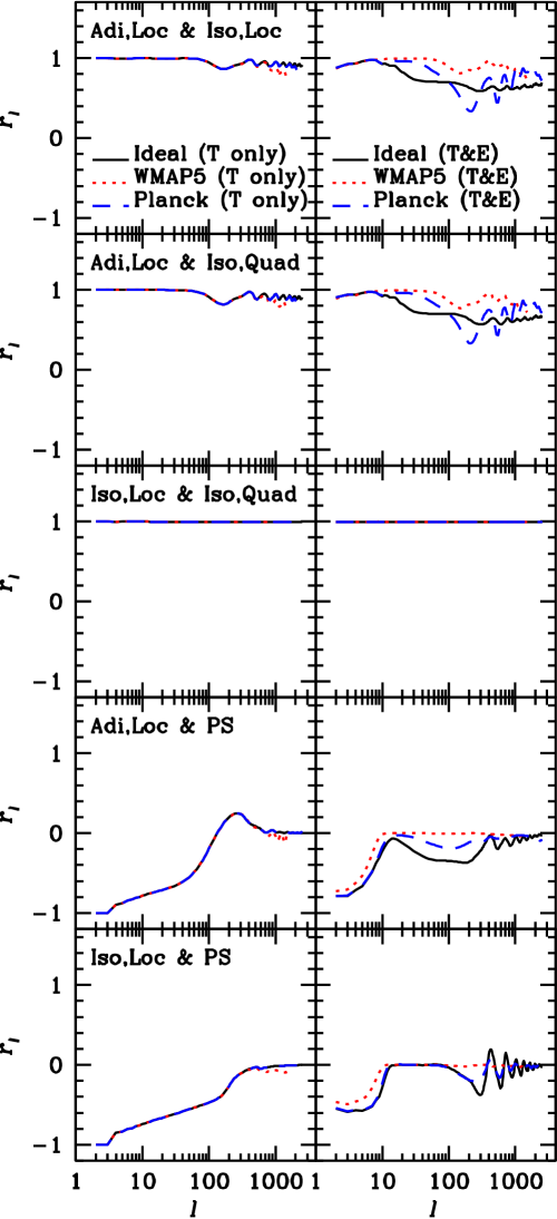
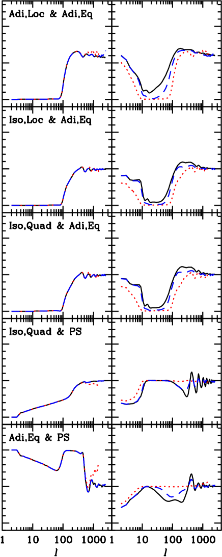
Figure 2: Cross-correlation coefficients $r_{l}^{ij}\equiv F_{l}^{ij}/(F_{l}^{ii}F_{l}^{jj})^{1/2}$ where $i$ and $j$ denote the local-type adiabatic (Adi,Loc), the local-type isocurvature (Iso,Loc), the equilateral-type adiabatic (Adi,Eq), the quadratic-type isocurvature (Iso,Quad), and the point source (PS) components. Left of each panel is temperature T only; right is T+E, including E polarization. Noise/Beam is for Ideal (solid), WMAP5 (dotted) and Planck observations (dashed).

Figure 3 shows 1$\sigma$ error contours (Cramér-Rao bound) for a pair of NG parameters for WMAP5 (T only), Planck (T only), and Planck (T&E). The errors expected from WMAP5 (T&E) is almost same as those from WMAP5 (T only). The rest of NG parameters other than two plotted are fixed to be zero. The local-type adiabatic and isocurvature components are correlated with the correlation coefficient $r=0.43$ for WMAP5, $r=0.23$ for Planck T only, $r=0.20$ for Planck T&E when $l$ is summed up to 2500. We see that the local-type and the quadratic-type scale-invariant isocurvature components are difficult to be differentiated even using Planck data. The local-type and the equilateral-type adiabatic components are weakly correlated ($r=0.12$ for WMAP5, $r=0.17$ for Planck T only, $r=0.22$ for Planck T&E), which is consistent with the previous work (Babich, Creminelli & Zaldarriaga, 2004). The point source component is almost uncorrelated with the other primordial components ($r<0.08$ for WMAP5 and $r<0.03$ for Planck), which is consistent with the previous work (Komatsu & Spergel, 2001). Table 2 lists the errors of the NG parameters without and with correlations among all of other parameters except for the quadratic-type isocurvature component. Polarization maps are found to be very important to constrain the isocurvature NG as well as adiabatic NG. The increase of the errors due to the correlations mainly between adiabatic and isocurvature modes is 20-30% for WMAP5, but less than 5% for Planck observations.

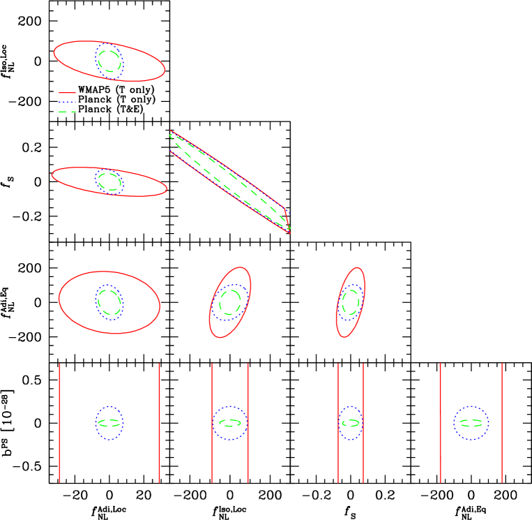
Figure 3: 1$\sigma$ error contours of a pair of NG parameters expected from WMAP5 T only (solid circles), Planck T only (dotted circles), and Planck T&E (dashed circles). The rest of NG parameters other than two plotted are fixed to be zero.

Table 2: 1$\sigma$ errors of each NG parameter from the joint analysis of all of the NG components except for the quadratic-type isocurvature components. The values without parentheses denote the limits with other parameters fixed, but those with parentheses denote the limits including the correlations such that the other parameters are marginalized.

	WMAP5		Planck
	T only		T only	T&E
$\Delta f_{\rm NL}^{\rm Adi,Loc}$	19 (23)		5.2 (5.5)	4.1 (4.3)
$\Delta f_{\rm NL}^{\rm Iso,Loc}$	59 (82)		57 (62)	34 (35)
$\Delta f_{\rm NL}^{\rm Adi,Eq}$	117 (149)		66 (71)	46 (48)
$\Delta b^{\rm PS}[10^{-28}]$	438 (441)		0.13 (0.13)	0.024 (0.024)

4 Summary

We have presented a detailed analysis of the possibility of extracting information about non–Gaussianity from various inflationary models. We consider four different-type primordial NG models: local-type adiabatic, equilateral-type adiabatic, local-type isocurvature, and quadratic-type isocurvature models together with point source contamination. The adiabatic and the isocurvature modes are correlated, but the difference in the phase of the corresponding acoustic oscillations breaks the degeneracy. The local-type and quadratic-type scale-invariant isocurvature components are difficult to separate even using Planck data. The correlation between the local-type and the equilateral-type adiabatic modes is weak. The point source (white noise) contamination does not pose a threat as it is uncorrelated with any of the $f_{\rm NL}$ parameters, although a high-resolution experiment will be more suited to get rid of such contamination. Our results are based on noise models from WMAP and Planck and we compare them to ideal noise-free and all-sky reference observations. The increase of the error for the non-Gaussian parameters due to the correlations is 20-30% for WMAP5 and 5% for Planck.

Secondary anisotropies other than point sources can contaminate the estimation of primordial non–Gaussianity. The cross-contamination of various inflationary contributions against secondaries such as Sunyaev-Zeldovich effect (SZ) or Integrated Sachs-Wolfe effect (ISW) which are potentially observable with Planck data will be present elsewhere.

References

- Acquaviva et al. (2003) Acquaviva V., Bartolo N., Matarrese S., Riotto A., 2003, Nucl. Phys. B667, 119
- Alishahiha, Silverstein & Tong (2004) Alishahiha M., Silverstein E., Tong T., 2004, Phys. Rev. D70, 123505
- Arkani-Hamed et al. (2004) Arkani-Hamed N., Creminelli P., Mukohyama S., Zaldarriaga M., 2004, JCAP, 0404, 001
- Babich & Zaldarriaga (2004) Babich D., Zaldarriaga M. 2004, Phys. Rev. D70, 083005
- Babich, Creminelli & Zaldarriaga (2004) Babich D., Creminelli P., Zaldarriaga M. 2004, JCAP, 8, 9
- Bartolo et al. (2004) Bartolo N., Matarrese S., Riotto A., 2004, Phys. Rev. D69, 043503
- Bartolo et al. (2004) Bartolo N., Komatsu E., Matarrese S., & Riotto A. 2004, Phys. Rept., 402, 103
- Bartolo, Matarrese & Riotto (2006) Bartolo N., Matarrese S., Riotto A., 2006, JCAP, 06, 024
- Bean et al. (2006) Bean R., Dunkley J., Pierpaoli E., 2006, Phys. Rev. D, 74, 063503
- Beltran (2008) Beltran M., 2008, Phys. Rev. D78, 023530
- Boubekeur & Creminelli (2006) Boubekeur L., Creminelli P., 2006, Phys. Rev. D73, 103516
- Boubekeur & Lyth (2006) Boubekeur L., Lyth D. H., 2006, Phys. Rev. D73, 021301
- Cabella et al. (2006) Cabella P., Hansen F. K., Liguori M., Marinucci D., Matarrese S., Moscardini L., Vittorio N., 2006, MNRAS, 369, 819
- Chen, Easther & Lim (2007) Chen X., Easther R., Lim E. A., 2007, JCAP, 0706, 23
- Creminelli et al. (2006) Creminelli P., Nicolis A., Senatore L., Tegmark M., Zaldarriaga M., 2006, JCAP, 5, 4
- Creminelli, Senatore, & Zaldarriaga (2007) Creminelli P., Senatore L., Zaldarriaga M., 2007, JCAP, 3, 19
- Dunkley et al. (2009) Dunkley J. et al., 2009, ApJS, 180, 306
- Dvali, Gruzinov & Zaldarriaga (2004) Dvali, G., Gruzinov, A., Zaldarriaga, M., 2004, Phys. Rev. D, 69, 083505
- Falk et al. (1993) Falk T., Madden R., Olive K. A., Srednicki M., 1993, Phys. Lett. B318, 354
- Gangui et al. (1994) Gangui A., Lucchin F., Matarrese S., Mollerach S., 1994, ApJ, 430, 447
- Gupta et al. (2002) Gupta S., Berera A., Heavens A. F., Matarrese S., 2002, Phys. Rev. D66, 043510
- Heavens (1998) Heavens A. F., 1998, MNRAS, 299, 805
- Hikage et al. (2009) Hikage C., Koyama K., Matsubara T., Takahashi T., Yamaguchi M., 2009, MNRAS accepted, preprint (arXiv:0812.3500)
- Kawasaki et al. (2008) Kawasaki M., Nakayama K., Sekiguchi T., Suyama T., Takahashi F., 2008, JCAP, 11, 19
- Kawasaki, Nakayama & Takahashi (2009) Kawasaki M., Nakayama K., Takahashi F., 2009, JCAP, 1, 2
- Komatsu & Spergel (2001) Komatsu E., Spergel D. N., 2001, Phys. Rev. D63, 3002
- Komatsu, Spergel & Wandelt (2005) Komatsu E., Spergel D. N., Wandelt B. D., 2005, ApJ, 634, 14
- Komatsu (2002) Komatsu, E., preprint (astro-ph/0206039)
- Komatsu et al. (2009) Komatsu E., et al., 2009, ApJS, 180, 330
- Koyama et al. (2007) Koyama K., Mizuno S., Vernizzi F., Wands D., 2007, JCAP 11, 24
- Langlois, Vernizzi & Wands (2008) Langlois D., Vernizzi F., Wands D., 2008, JCAP, 12, 4
- Liguori et al. (2007) Liguori M., Yadav A., Hansen F. K., Komatsu E., Matarrese S., Wandelt B., 2007, Phys. Rev. D76, 105016
- Linde & Mukhanov (1997) Linde A. D., Mukhanov V., 1997, Phys. Rev. D56, R535
- Lyth, Ungarelli & Wands (2003) Lyth D. H., Ungarelli C., Wands D., 2003, Phys. Rev. D67, 023503
- Maldacena (2003) Maldacena J. M., 2003, JHEP, 5, 13
- Medeiros & Contaldi (2006) Medeiros J., Contaldi C. R., 2006, MNRAS, 367, 39
- Moroi & Takahashi (2009) Moroi T., Takahashi T., 2009, Phys. Lett. B, 671, 339
- Moss & Xiong (2007) Moss I., Xiong C., 2007, JCAP, 0704, 007
- Munshi & Heavens (2009) Munshi D., Heavens A., 2009, preprint (arXiv:0904.4478)
- Peebles (1999) Peebles P. J. E., 1999, ApJ, 510, 531
- Salopek & Bond (1990) Salopek D. S., Bond J. R., 1990, Phys. Rev. D42, 3936
- Seery & Lidsey (2005) Seery D., Lidsey J. D., 2005, JCAP, 6, 3
- Seljak & Zaldarriaga (1996) Seljak, U., Zaldarriaga, M. 1996, ApJ, 469, 437
- Smith & Zaldarriaga (2006) Smith K. M., Zaldarriaga M., 2006, preprint (arXiv:astro-ph/0612571)
- Smith, Senatore & Zaldarriaga (2009) Smith K. M., Senatore L., Zaldarriaga M., 2009, preprint (arXiv:0901.2572)
- Suyama & Takahashi (2008) Suyama T., Takahashi F., 2008, JCAP, 9, 7
- Verde et al. (2000) Verde L., Wang L., Heavens A. F., Kamionkowski M., 2000, MNRAS, 313, 141
- Wang & Kamionkowski (2000) Wang L., Kamionkowski M., 2000, Phys. Rev. D61, 63504
- Yadav & Wandelt (2008) Yadav A. P. S., Wandelt B. D., 2008, Phys. Rev. Lett., 100, 181301
- Yadav, Komatsu,& Wandelt (2007) Yadav A. P. S., Komatsu E., Wandelt B. D., 2007, ApJ, 664, 680