Automated Determination of [Fe/H] and [C/Fe] from Low-Resolution Spectroscopy

Abstract

We develop an automated spectral synthesis technique for the estimation of metallicities ([Fe/H]) and carbon abundances ([C/Fe]) for metal-poor stars, including Carbon-Enhanced Metal-Poor (CEMP) stars, for which other methods may prove insufficient. This technique, autoMOOG, is designed to operate on relatively strong features visible in even low- to medium-resolution spectra, yielding results comparable to much more telescope-intensive high-resolution studies. We validate this method by comparison with 913 stars which have existing high-resolution and low- to medium-resolution spectra, and that cover a wide range of stellar parameters. We find that at low metallicities ([Fe/H] $\lesssim-2.0$), we successfully recover both the metallicity and carbon abundance, where possible, with an accuracy of $\sim 0.20$ dex. At higher metallicities, due to issues of continuum placement in spectral normalization done prior to the running of autoMOOG, a general underestimate of the overall metallicity of a star is seen, although the carbon abundance is still successfully recovered. As a result, this method is only recommended for use on samples of stars of known sufficiently low metallicity. For these low-metallicity stars, however, autoMOOG performs much more consistently and quickly than similar, existing techniques, which should allow for analyses of large samples of metal-poor stars in the near future. Steps to improve and correct the continuum placement difficulties are being pursued.

1. INTRODUCTION

One of the most intriguing results from modern surveys of metal-poor stars, such as the HK (Beers et al., 1985, 1992) and Hamburg/ESO surveys (HES; Christlieb et al., 2001), is the large fraction of Carbon-Enhanced Metal-Poor (CEMP; [C/Fe] $\geq+1.0$) stars identified amongst the lowest metallicity stars. The exact fraction of CEMP stars at low metallicity has been debated in the literature, and is variously reported as $\sim$10% (Frebel et al., 2006), $\sim$15% (Cohen et al., 2005) or $\sim$20% (Lucatello et al., 2006) of stars with [Fe/H] $\leq-2.0$; $\sim$20%-25% of stars with [Fe/H] $\leq-2.5$ (Marsteller et al., 2005); or nearly 40% of stars with [Fe/H] $\leq-3.5$ (Beers & Christlieb, 2005). The fraction of CEMP stars is expected, on theoretical grounds, to increase with declining metallicity (Tumlinson, 2007). The evolutionary states of sample stars can also play a significant role, due to the mixing-induced dilution of carbon (Aoki et al., 2006; Lucatello et al., 2006).

To better specify the changing CEMP fraction with metallicity, much larger samples of stars are required. Existing studies have generally been limited to (small) samples of low-metallicity stars for which high-resolution spectral abundances have been obtained (with the exception of Frebel et al., 2006). Such spectra are time consuming to obtain and simply fail to exist in large enough samples. Lower-resolution spectra are available in sufficient quantity, but the techniques used to determine abundances are more inconsistent across parameter space, and largely based on empirical calibrations (e.g., Beers et al., 1999; Rossi et al., 2005).

Here we discuss the development of an automatic spectral synthesis fitting routine, autoMOOG, which enables rapid spectral fitting of the low- to medium-resolution spectra available in existing and future large samples of metal-poor stars. Papers in preparation will use this technique, and others, on a much larger sample of stars than has been studied to date, to determine the frequency of carbon enhancement as a function of metallicity. autoMOOG will also be vital for identifying the most useful and interesting targets from large data sets for future high-resolution follow-up.

This paper is outlined as follows. Section 2 presents a discussion of the current techniques and a description of the new method that has been developed. Error analysis, performed on the program using synthetic spectra, is presented in Section 3. Section 4 considers validation of the autoMOOG approach using medium-resolution spectra of stars with available high-resolution determinations of [Fe/H] and [C/Fe]. The important question of the specification of upper limits on [C/Fe] for warmer stars (where the prominent C features are quite weak) is addressed in Section 5. Section 6 presents brief conclusions and a discussion of future work anticipated for refinement of autoMOOG.

2. METHODOLOGY

For metal-poor stars with only low- to medium-resolution spectroscopy available, stellar parameters such as metallicity ([Fe/H]) and carbon abundance ([C/Fe]) have primarily been estimated from broadband colors and line indices measuring the strength of the Caii K line and the CH $G$ band–the KP and GP indices, respectively (Beers et al., 1999; Rossi et al., 2005). However, for CEMP stars, the presence of strong carbon features may affect the measured colors of a star, in particular the $B$ magnitude. Rossi et al. (2005) have attempted to account for this by using $J-K$ colors instead of $B-V$ used by Beers et al. (1999). Strong carbon features may also affect the measurement of the continuum in a side band of the KP index (as first indicated by Cohen et al., 2005). Such effects could lead to an underestimation of the stellar metallicity. Very strong carbon features can also “overflow” into the sidebands used for the measurement of the GP index, confounding estimates of [C/Fe].

It is useful to explore different approaches that should be relatively immune to these effects. One such method involves the use of model stellar atmospheres to generate synthetic spectra, so that detailed fits of a given observed spectrum may be made, rather than suffer the loss of information inherent in techniques based on line indices. We have explored using the spectrum analysis code MOOG (Sneden, 1973), a grid of ATLAS9 1D, LTE stellar atmosphere models and atomic and molecular line lists (including lines of CH, CN, and C₂; Castelli & Kurucz, 2003) to carry out this approach. We have developed a routine to automatically run MOOG and minimize the residuals of the resulting model spectra when compared against certain critical regions of the observed data.

Using the line index methods in concert with other techniques (see Lee et al., 2006), T_eff and log $g$ values are adopted and initial estimates are determined for [Fe/H] and [C/Fe]. From our grid of models (with spacing of 100 K in T_eff, 0.2 in log $g$, and 0.5 in [M/H], or overall solar-scaled metallicity), we select the model that most closely matches our starting parameters. This model is used within MOOG, where individual abundances are then varied to the nearest 0.05 dex to fit a full line profile. If the metallicity is varied significantly, the next appropriate model in the grid is used instead. Any element not currently being fit is given the model solar-scaled value. However, the user may specify other individual elements to vary as well, generally by a fixed offset from the scaled value. Thus, for example, it would be possible to use CH to determine [C/Fe], and then use that value to fit CN to determine [N/Fe].

As in the line index method, the Ca ii K line at 3933 Å is used to solve for the metallicity of a star. At low- to medium-resolution, no iron lines are strong enough to be cleanly measured, so calcium is used as a proxy for metallicity. However, unlike the line index method, which empirically calibrates the strength of the KP index to the metallicity, here the Ca ii K line is fit to obtain a calcium abundance. Since calcium is an $\alpha$-element, an appropriate, metallicity-dependent offset, to account for possible $\alpha$-enhancements, must be used when determining the metallicity of a star. Following Beers et al. (1999), we use an $\alpha$-enhancement applicable for Milky Way stars of:

$$[\alpha/\textrm{Fe}]=\left\{\begin{array}[]{ll}0&\textrm{if [Fe/H]}\geq 0\\ -0.267*[\textrm{Fe/H}]&\textrm{if}-1.5\leq[\textrm{Fe/H}]<0\\ 0.4&\textrm{if [Fe/H]}<-1.5\\ \end{array}\right.$$ (1)

The initial guess for [C/Fe] is also included in our metallicity fit to address the effect pointed out by Cohen et al. (2005).

Using the new, more precisely determined metallicity, [C/Fe] can similarly be fit using the CH $G$ band at 4304 Å. However, for warmer stars, those with a lower carbon abundance, or those that are very metal-poor, the $G$ band may be too weak to be detected. In these cases, an upper limit for [C/Fe] is determined instead. In theory, with an updated [C/Fe], it may be necessary to iterate on the fit to the Ca ii K line. However, extensive testing revealed that the metallicity determined using the input [C/Fe] and that obtained from the refined [C/Fe] varied by negligible amounts (if at all), suggesting that such iteration is not required at this precision.

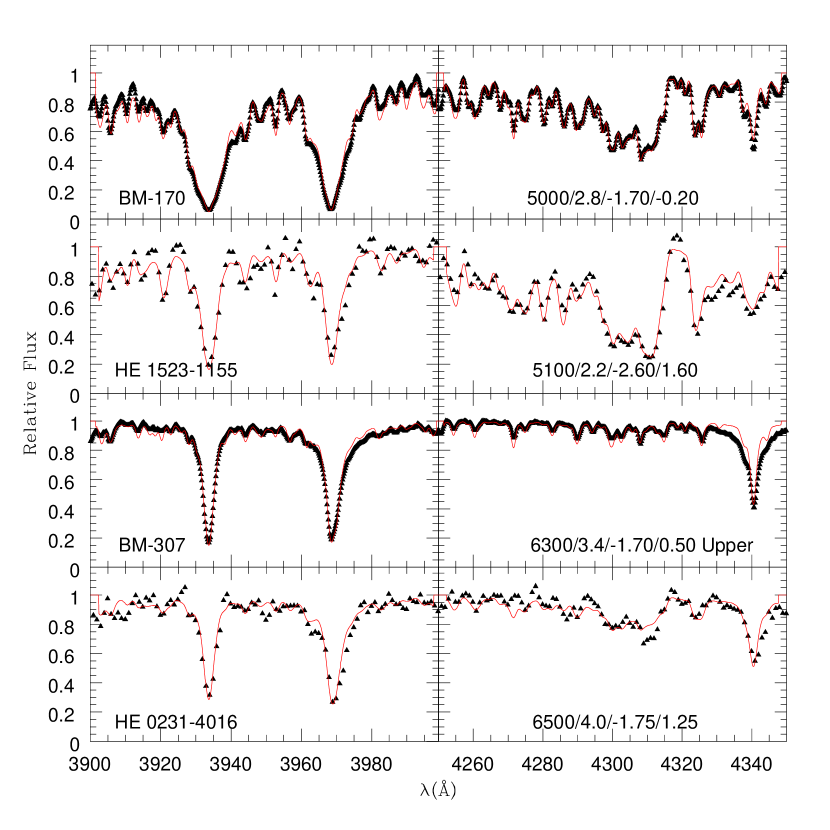
Figure 1.— Example of the fits (line) produced by autoMOOG of the Ca ii K region (left) and of the $G$ band (right) compared to the data (triangles). The numbers in the right panels correspond to the T_eff, log $g$, [Fe/H], and [C/Fe], respectively, of the star. Note the higher resolution of the BM stars compared to the HERES sample, showing that a range of spectral resolutions can easily be fit. These stars also show the effect of temperature and abundances on the appearance of the Ca ii K line and the $G$ band, as well as the appearance of an upper limit determination.

Once this approach was worked out by fitting the abundances of a number of stars by hand, a program, autoMOOG, was developed to iteratively vary abundances and automatically minimize the $\chi^{2}$ of the synthetic spectra produced by MOOG. autoMOOG allows the user to select any wavelength region for the comparison. For the results presented here, a fit was determined using the ranges 3910$-$3960 Å for the Ca ii K line, and 4275$-$4330 Å for the CH $G$ band. An example of the fits produced by autoMOOG can be seen in Figure 1.

As part of the automation, autoMOOG also uses the region around the Ca ii K line to estimate the observed radial velocity, which is used to align the data with the model spectra. The velocity precision is directly proportional to the spectral resolution, which for our test spectra ($R\sim 4000$) is typically $\lesssim$10 km s^-1. Continuum subtraction and spectral renormalization occur prior to the running of autoMOOG. Assuming this renormalization to be valid, autoMOOG applies a small additive offset to the local continuum level of the normalized, continuum-subtracted observed spectra such that it matches the local continuum level of the comparison synthetic spectra without altering the effective line strength. As we will see in Section 4, this assumption likely becomes less valid at higher metallicities, where the apparent continuum is significantly suppressed in the vicinity of the Ca ii line, leading to incorrect continuum subtraction.

3. ERROR ANALYSIS

To estimate the errors on the derived abundances, a set of noiseless synthetic spectra across the grid of parameters was generated. Since these spectra had known parameters, the abundance determinations could be directly compared with the proper values. These spectra were first run through autoMOOG to determine any intrinsic scatter in the estimates. These errors, and their rough dependence on T_eff and log $g$, are listed in Table 1. The errors are roughly constant across both of these parameters, with the exception of very cool giants where the scatter increases. Also, note that the minimum errors are limited by the resolution of the abundance grid (0.05 dex).

Table 1Abundance Errors, and Their Dependence on T_eff and log $g$

	[Fe/H]					[C/Fe]
Bin	$\sigma_{\mathrm{Int}}$	$\sigma_{\mathrm{T}_{eff}}$	$\sigma_{\mathrm{log}g}$	$\sigma_{\mathrm{Total}}$		$\sigma_{\mathrm{Int}}$	$\sigma_{\mathrm{T}_{eff}}$	$\sigma_{\mathrm{log}g}$	$\sigma_{\mathrm{Total}}$
Errors in Bins of Teff
4000 K	0.162	0.306	0.236	0.351		0.267	0.238	0.207	0.267
5000 K	0.058	0.168	0.073	0.174		0.058	0.107	0.064	0.111
6000 K	0.093	0.139	0.070	0.139		0.088	0.097	0.065	0.097
7000 K	0.041	0.123	0.046	0.125		0.033	0.104	0.085	0.130
Errors in Bins of log $g$
4.0	0.124	0.172	0.112	0.172		0.153	0.153	0.119	0.153
4.6	0.139	0.154	0.139	0.154		0.152	0.161	0.141	0.161
5.0	0.180	0.254	0.172	0.254		0.174	0.168	0.143	0.174

The intrinsic errors are nonzero due to the nature of the abundance determination. The program must first determine a cross-correlation velocity and continuum level in order to shift the data to match the model spectra. The finite resolution of the data and model spectra, as well as the finite grid of velocity shifts and input model abundances, occasionally leads to small offsets in abundance determinations. The uncertainty introduced by these various fitting steps, including the velocity and continuum shift, as well as other sources of error, are then included in the observed intrinsic scatter. Note, however, that this scatter is still quite small.

Since external values for T_eff and log $g$ are adopted in choosing a model, appropriate errors in these parameters ($\sigma_{\mathrm{T}_{eff}}$ = 200 K, $\sigma_{\mathrm{log}g}$ = 0.4; Lee et al, 2008) need to be translated into errors on the abundances. Since [Fe/H] and [C/Fe] are fit internally, using the external values only as a starting point, the errors on these parameters do not need to be considered.

To translate these errors, the same synthetic spectra used to determine the intrinsic error were refit with incorrect stellar parameters ($\pm$100, $\pm$200 K in T_eff, and $\pm$0.2, $\pm$0.4 in log $g$, which correspond to the line index errors and are related to the spacing of the model grid). The resulting combined errors for [Fe/H] and [C/Fe] based on the uncertainties in these parameters and the intrinsic errors are shown in Table 1. Total errors are then estimated from these individual sources by assuming approximate Gaussian distributions. Since the errors are essentially constant across log $g$, the total errors are most reasonably read from the bins of varying temperature, and are thus less than $\sim$ 0.20 dex for [Fe/H] and $\sim$ 0.15 dex for [C/Fe], for stars warmer than 4000 K.

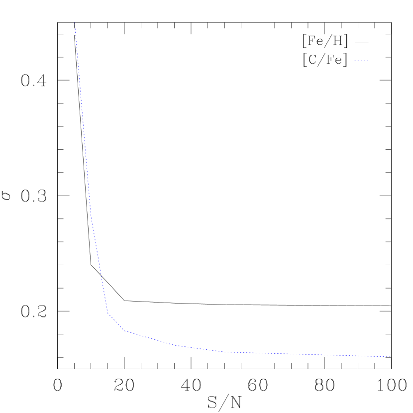
Figure 2.— Total error for [Fe/H] (solid line) and [C/Fe] (dotted line) vs. signal-to-noise ratio.

The error in the abundances due to the changing signal to noise of the data also needs to be considered. To determine this, varying amounts of noise were injected into the noise-free synthetic spectra, which were run through autoMOOG again. This error combined with the previous errors (assuming $\sigma_{\mathrm{[Fe/H]}}=0.20$ dex and $\sigma_{\mathrm{[C/Fe]}}=0.15$ dex) are shown in Figure 2. The total errors are then less than 0.25 dex for S/N $\gtrsim$ 10 for both [Fe/H] and [C/Fe].

4. VALIDATION

Validation of the autoMOOG approach requires comparison of the results, as obtained from medium-resolution spectra, with stars that have abundances determined from high-resolution analyses. Differences between high-resolution and lower-resolution analyses, such as differences in adopted stellar parameters, different lines used for individual abundances, and differences in fitting techniques, may all lead to small scatter between results. However, lower-resolution techniques are often empirically calibrated to higher-resolution studies, which somewhat mitigates this scatter. Comparison of the autoMOOG technique with other methods designed for lower-resolution spectra, such as the line index method, would also be valuable, particularly since they would be looking at the same features. These comparisons are performed for two sets of data, as described below.

4.1. The Data

The first set of stars analyzed are from the catalog of Bidelman & MacConnell (1973, hereafter BM), originally identified as metal-weak candidates in the southern sky. This sample ranges from around [Fe/H] = $-2.5$ up to solar metallicity, and thus represents a modestly metal-poor, and predominantly carbon-normal, sample. The high-resolution values used here come from the literature compilation of Cayrel de Strobel et al. (2001). The medium-resolution ($\sim 1$ Å, S/N $\sim 100$) spectra that are being fit are described in T. C. Beers et al (2009), in preparation.

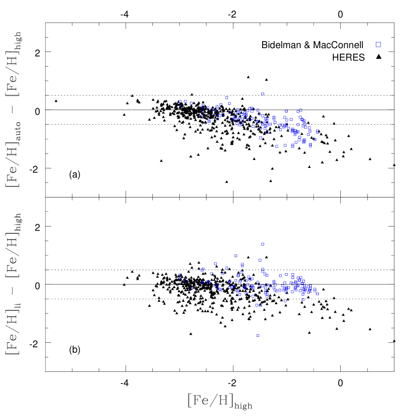
Figure 3.— Comparisons of the metallicity determined from (a) autoMOOG and (b) the line index method to the high-resolution results. In both cases, the higher metallicity, carbon-normal BM stars are plotted as open squares, while the more metal-poor, occasionally carbon-rich HERES stars are plotted as filled triangles. The solid line corresponds to agreement with the various abundances. The dashed lines to either side correspond to a difference of $\pm$0.5 dex.

The other data are a sample of metal-poor stars observed as part of the Hamburg/ESO R-process Enhanced Star survey (HERES; Christlieb et al., 2004). Initially selected from the full Hamburg/ESO and HK surveys, the HERES project obtained moderate-resolution ($\sim 2$ Å) follow-up spectroscopy for metal-poor giant candidates. For bright stars confirmed to have [Fe/H] $<-2.5$, higher-resolution ($R=20,000$, S/N $\sim 50$, $\lambda=3760-4980$ Å) spectroscopy was obtained (Barklem et al., 2005; Lucatello et al., 2006). Their goal was to identify the small fraction of these stars that showed large enhancements of r-process elements, so that investigations into the nature of this process could be conducted. As a consequence of these observations, several hundred metal-poor stars, many of them carbon-enhanced, were observed at moderate and high resolution.

These then make ideal samples for the present analysis, as the medium-resolution data can be run through autoMOOG, and the high-resolution results are available for the purposes of comparison.

4.2. Results

Due to the high quality spectra available for the majority of the medium-resolution data, metallicities and carbon abundances were determined for nearly all the stars in the samples. A total of 913 stars were fit, including 529 from the BM sample and an additional 384 from the HERES sample. In some cases, stars had no metallicity determination available from the line index method. In addition, many of the BM stars lacked high-resolution metallicities, and almost none had high-resolution carbon abundances. In all of these cases, abundances were obtained using autoMOOG, but obviously no comparison was possible.

When comparing autoMOOG results for metallicity with the high-resolution analysis (Figure 3a), it can be seen that there exists a generally good agreement at low metallicities, with a small scatter and no appreciable offset. Due to issues of continuum placement in the normalization of higher metallicity ([Fe/H] $\gtrsim-2.0$) input spectra, an increasing underestimate of metallicity is seen.

During the process of continuum subtraction and spectral normalization prior to the running of autoMOOG, a continuum is placed along the apparent continuum of a stellar spectrum. For high-metallicity stars observed at low spectral resolution, the multitude of metallic lines causes a suppression in the apparent continuum, masking the true continuum level. Continuum subtraction techniques will improperly normalize such spectra, and subsequent lines fit within autoMOOG, such as calcium, will then appear weaker than they truly are, resulting in a general underestimate in the metallicity estimates.

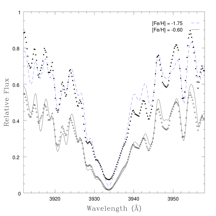
Figure 4.— Synthetic spectrum near the Ca II K line assuming [Fe/H] = $-1.75$ (dashed line) and [Fe/H] = $-0.60$ (solid line) for a star of T_eff = 4800, log $g$ = 2.2. Overplotted are points corresponding to data from a star in the BM sample, using the data created after the continuum fit (filled triangles) and that same data scaled to match the solid line (open triangles). Note the different apparent continuum levels for the metal-poor spectrum vs. the metal-rich spectrum.

This effect is demonstrated in Figure 4. Synthetic spectra are plotted for models with T_eff = 4800 K and log $g$ = 2.2, with possible metallicities of [Fe/H] = $-1.75$ (dashed line) and [Fe/H] = $-0.60$ (solid line). Overplotted on these synthetic spectra are the data from star CD-57:949, taken from the BM sample. The filled triangles correspond to the flattened, normalized spectrum as produced from the continuum fit to the data. The open triangles, on the other hand, are the same data after application of a scaling factor selected to best match the higher metallicity synthetic spectra. Based on the input, filled triangle spectra, autoMOOG appropriately selected a metallicity of [Fe/H] = $-1.75$ for this star. The fit is far from perfect, but is the best fit to the input spectrum. The filled triangles are clearly better matched by the dashed line than they are by the solid line.

However, the higher metallicity synthetic spectrum, at [Fe/H] = $-0.60$, is close to the actual metallicity of CD-57:949, as determined from high-resolution analyses. If the data were more appropriately scaled, as with the open triangles, it would better match this spectrum. Even in this rough simulation, it is fairly clear that the open triangles match the solid line much better than the filled triangles match the dashed line. However, from the data supplied to autoMOOG, an incorrect, and always lower metallicity, synthetic spectrum is chosen as the best fit. This problem becomes more severe at higher metallicities as the apparent continuum is further suppressed relative to the true continuum, resulting in larger deviations to lower selected metallicities. Thus, this is a problem with the input spectra, not with autoMOOG itself. With properly continuum-subtracted spectra, autoMOOG will likely produce results with similar scatter seen at low metallicity.

Efforts have been made to include renormalization within autoMOOG to attempt to deal with this problem. While renormalization does show some promise, its results are currently erratic. Future versions of autoMOOG will likely include renormalization, but it will take considerable modifications to the code before this becomes a stable feature.

The line index results (Figure 3b) exhibit more scatter than autoMOOG at low metallicity, but similar behavior at high metallicity. For the line index approach at high metallicity, this is caused in part by the same continuum issues mentioned above but also by saturation of the KP index. This can occasionally be minimized by substitution of other metallicity determination methods designed specifically to handle higher metallicity stars, such as the auto-correlation function suggested by Ratnatunga & Freeman (1989) and explored by Beers et al. (1999). This accounts for the smaller deviations from the high-resolution results of the BM stars, but not the HERES stars, seen in the line index comparison plot. Also note that the stars with [Fe/H] $\lesssim-1.0$ that show the largest deviations in Figure 3a are simply not present in Figure 3b, as the line index method failed to determine any metallicity for these stars.

As such, metallicities determined with autoMOOG are generally as good as those determined using existing techniques, and somewhat better at the lowest metallicities ([Fe/H] $<-3.0$). Since this method was designed for use with VMP stars, it is then better than existing techniques at accurately determining metallicities. However, due to the difficulties at higher metallicity, it should not be used blindly with samples that may contain stars with metallicity greater than about [Fe/H] = $-2.0$.

Much better agreement is seen when comparing the autoMOOG fits on carbon, [C/Fe], to the high-resolution abundances (Figure 5). The only stars plotted are those for which fits (as opposed to upper limits) have been obtained and for which high-resolution abundances are available. When plotted as a function of [C/Fe] (Figure 5a), it is seen that there is very little scatter at lower [C/Fe] and only slightly larger scatter as the carbon abundance is increased. At higher carbon abundances, the added scatter is likely due to the presence of other strong carbon features in the vicinity of the $G$ band, or the decreased sensitivity of the $G$ band as it begins to saturate.

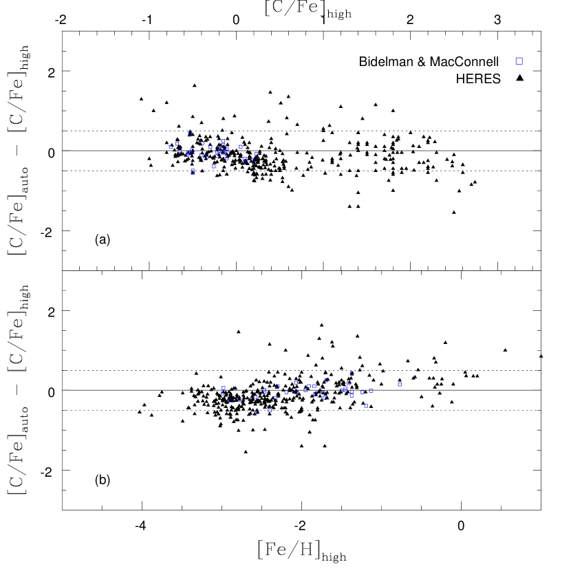
Figure 5.— Comparisons of the carbon abundance, [C/Fe], determined from autoMOOG to that determined from high-resolution analyses, plotted vs. the high-resolution (a) [C/Fe] and (b) [Fe/H]. The points are the same as in Figure 3. Upper limits are not plotted, only determined values.

Examination of the carbon fits as a function of metallicity (Figure 5b) indicates little scatter, but a small slope seems to be present. This slope is not real, but is caused by a jump at [Fe/H] $\sim-2.5$, with a slight underestimation of [C/Fe] at lower metallicities, and a slight overestimation at higher metallicities. The underestimation at low metallicity is likely caused by the use of different carbon features at high and low resolution, which are affected differently by model atmosphere parameters (i.e., one-dimensional versus three-dimensional and LTE versus NLTE). This then should extend to higher metallicities as well, for a global underestimation of around 0.25 dex.

The slight overestimation of [C/Fe] at high metallicity is likely caused by the same difficulties that have already been seen at high metallicity, although the effect is much weaker here. The reason for this weaker effect is that the carbon fits are actually a fit of [C/M], where M is the scaled-solar model abundance. To ultimately derive [C/Fe], this model-dependent carbon value needs to be offset by the deviation of iron from the model. This offset is at most half of the distance between models in our grid (i.e., $\Delta$[Fe/H] $\leq 0.25$ dex), and thus should not significantly affect the final results, but causes this slight relative overestimation.

In addition, the temperatures used were determined from photometric colors. At times, the parameters adopted for the high-resolution analysis vary from these values, occasionally up to a difference of nearly 1000 K, although generally only by a few hundred kelvin. As seen in Section 3, such offsets in temperature could lead to offsets in metallicity of $\sim$0.15 dex and $\sim$0.10 dex in [C/Fe]. Due to the inconsistent nature of these offsets, this could also lead to enhanced scatter in any of the comparisons to high resolution.

It is also possible to use these results to perform an internal consistency check on the method. Since a number of stars from the BM sample have been observed multiple times at medium resolution, the abundances determined for each individual spectra can then be compared to see if autoMOOG determines the same relative abundances for a given star, regardless of the spectra used. For each star, an average metallicity and carbon abundance are calculated from the available results, and then the residuals between each individual abundance and the average are calculated.

For both metallicity and carbon abundance, a very small scatter around zero of $\sim$ 0.02 dex is observed, well within the intrinsic errors, showing the overall stability of autoMOOG. The scatter for [Fe/H] at high metallicities may be slightly larger than elsewhere. This is assumed to be a result of the exact continuum fit used for each spectra, and is thus associated with the general high-metallicity difficulties. Even so, this scatter is still quite small, increasing by no more than 0.01 dex.

5. UPPER LIMITS

For the purpose of this work, a $G$ band is considered detectable if its deflection from the continuum is at least 5% the value of the continuum at that position. Upper limits for [C/Fe] were determined by varying abundances of synthetic spectra and comparing their strengths against an essentially “zero” carbon abundance spectrum which was used to set the continuum level. A surface in T_eff-log $g$ space was then fit to these values. Stars with carbon abundances below this surface were reassigned with the value of the upper limit at that position, and flagged appropriately. The approximate position of this cutoff can be seen in Figure 6.

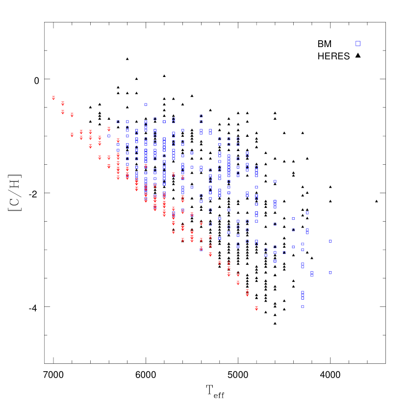
Figure 6.— Carbon abundances ([C/H]) plotted vs. effective temperature. Plotted are the abundances for the BM sample (open squares) and the HERES sample (filled triangles). All upper limits are denoted with an arrow.

When the $G$ band can be properly fit, appropriate [C/Fe] values are generally determined. It is, however, useful to explore under what physical conditions only an upper limit is obtained. The detectability of the $G$ band relative to temperature and metallicity is shown in Figures 6 and 7, respectively.

In Figure 6, the carbon abundance, [C/H], is plotted versus effective temperature using the values from autoMOOG. The stars in these samples cover a fairly wide range of temperatures, from 4000 K to 7000 K. Both samples of stars cover about the same temperature range.

The $G$ band is a molecular feature, which, for the same abundance of carbon, will appear stronger at lower temperatures. As temperature is increased, the $G$ band weakens until it is no longer detectable. The point where this happens is obviously dependent on the level of carbon enhancement, [C/H], and is easily seen in the plot. [C/H] is used for this analysis as it is solely a measure of the carbon abundance, without any implicit assumptions about overall metallicity, which, along with the temperature, is primarily what the strength of the $G$ band depends on. From the line of detectability, it can be seen that for cool stars, the $G$ band can essentially always be detected. However, for warm stars, especially above 6000 K, carbon abundances must be fairly high to be detected. Indeed, for temperatures above 7000 K, it would be difficult to measure a carbon abundance at all, no matter how high its true abundance. In part, this is due to the apparent upper limit on [C/H].

Although there are a handful of stars with slightly higher carbon abundances, a general limit to the allowed carbon abundances falling at [C/H] $\sim-0.5$ can be seen, which is higher than some have found ($-1.0$ and $-0.7$ : Ryan, 2003; Frebel et al., 2006, respectively), while lower than others (0.0 : Lucatello et al., 2005; Aoki et al., 2007). It is likely that the true location of this upper limit is temperature dependent, with cooler stars exhibiting a lower value, and warmer stars a higher value. This may be visible in Figure 6, and can further be supported by the previously mentioned results, and is presumably due to evolutionary effects.

Figure 7.— Metallicity distribution function for the full HERES and BM sample (solid line) and those stars for which only an upper limit on carbon have been determined (dashed line).

While the two samples we have examined do not fully complement each other, as seen in their combined Metallicity Distribution Function (MDF; Figure 7), their results can still be used to analyze the detectability of the G band with respect to metallicity. Figure 7 shows the MDF of the full samples of stars, and the MDF of stars with only a measured upper limit.

This second set of stars overall traces the shape of the full MDF, although accounting for slightly larger percentages of stars at lower metallicities. This is not surprising, as metal-poor stars have, by definition, low abundances and weak lines. However, due to the high quality of these samples, carbon abundances are able to be determined for a significant fraction of stars, even at the lowest metallicities.

6. CONCLUSIONS AND FUTURE WORK

We have developed a new method for the determination of [Fe/H] and [C/Fe] for stars using automated spectral synthesis. This method appears to not be affected by the presence of additional C-related features in the spectra of some stars that has been claimed by Cohen et al. (2005) to limit the accuracy of the line index method for CEMP stars, and does not require the massive calibration required by that method. autoMOOG is significantly quicker and more consistent than spectral synthesis by hand, which in general could vary from individual to individual, and even for one individual over the course of time.

We have explored the behavior of this method for two samples of stars with both medium-resolution and high-resolution spectroscopy available. Using this method on two samples of stars which cover a wide range of parameter space, we are able to see exactly how this method behaves. For stars with [Fe/H] $\leq-2.0$, both the metallicity, [Fe/H], and carbon abundance, [C/Fe], where detectable, are able to be successfully recovered. Despite the known problems with their metallicities, the carbon abundances for the more metal-rich stars are similarly recovered. As this method was designed and optimized primarily for use with metal-poor stars, it should not be used indiscriminately with samples containing more metal-rich samples, as these stars will contaminate metal-poor studies due to the metallicity underestimation. In future versions of this technique, we will attempt to resolve the issues present at high metallicity through implementation of various methodologies currently under development. However, at least for stars with [Fe/H] $\leq-2.0$, it is more consistently accurate (with errors of around 0.2 dex for both [Fe/H] and [C/Fe]) than previous abundance methods, especially at the lowest metallicities, where these other methods break down.

Although we do not show it here, this program is capable of fitting any element from any detectable line. Thus, it would be possible to, for instance, measure the abundance (or an upper limit) of s-process elements such as barium (4554 Å) or strontium (4078 Å), expected to be enhanced for many CEMP stars. In this way, we could roughly separate CEMP stars into the CEMP-s and CEMP-no classes (Beers & Christlieb, 2005). However, detailed studies of these fits have not yet been performed. In particular, no similar upper limit mechanism is in place for these other lines. For the moment, fitting other features should only be done for very rough estimates, and should not be used for any detailed science, but can be used for identification of likely neutron-capture enhanced targets for high-resolution follow-up. Future versions of autoMOOG will allow fitting for a larger variety of lines with more robust detection and saturation algorithms, as well as internal fitting of effective temperature and surface gravity, to provide less dependence on external techniques.

The authors are grateful to John Norris for permitting access to his spectroscopic observations of the Bidelman & MacConnell candidates prior to publication. B.M., T.C.B., and T.S. acknowledge partial support from grants AST 00-98508, AST 00-98549, AST 04-06784, and AST 07-07776, as well as PHY 02-16783 and PHY 08-22648, Physics Frontier Centers/JINA: Joint Institute for Nuclear Astrophysics, awarded by the US National Science Foundation. S.R. and V.P. acknowledge partial financial support from the Brazilian institutions FAPESP, CNPq and Capes. S.L. acknowledges partial support from INAF cofin 2006 and the DFG cluster of excellence ’Origin and Structure of the Universe’ (www.universe-cluster.de)

References

- Aoki et al. (2007) Aoki, W., Beers, T. C., Christlieb, N., Norris, J. E., Ryan, S. G., & Tsangarides, S. 2007, ApJ, 655, 492
- Aoki et al. (2006) Aoki, W., et al. 2006, ApJ, 639, 897
- Barklem et al. (2005) Barklem, P. S., et al. 2005, A&A, 439, 129
- Beers & Christlieb (2005) Beers, T. C., & Christlieb, N. 2005, ARA&A, 43, 531
- Beers et al. (1992) Beers, T. C., Preston, G. W., & Shectman, S. A. 1992, AJ, 103, 1987
- Beers et al. (1985) Beers, T. C., Preston, G. W., & Shectman, S. A. 1985, AJ, 90, 2089
- Beers et al. (1999) Beers, T. C., Rossi, S., Norris, J. E., Ryan, S. G., & Shefler, T. 1999, AJ, 117, 981
- Bidelman & MacConnell (1973) Bidelman, W. P., & MacConnell, D. J. 1973, AJ, 78, 687
- Castelli & Kurucz (2003) Castelli, F., & Kurucz, R. L. 2003, in IAU Symp. 210, Modelling of Stellar Atmospheres, ed. N. Piskunov, W. W. Weiss, & D. F. Gray (Dordrecht: Reidel Publishing), 20P
- Cayrel de Strobel et al. (2001) Cayrel de Strobel, G., Soubiran, C., & Ralite, N. 2001, A&A, 373, 159
- Christlieb et al. (2004) Christlieb, N., et al. 2004a, A&A, 428, 1027
- Christlieb et al. (2001) Christlieb, N., Green, P. J., Wisotzki, L., & Reimers, D. 2001, A&A, 375, 366
- Cohen et al. (2005) Cohen, J. G., et al. 2005, ApJ, 633, L109
- Frebel et al. (2006) Frebel, A., et al. 2006, ApJ, 652, 1585
- Lee et al (2008) Lee, Y. S., et al. 2008, AJ, 136, 2022
- Lee et al. (2006) Lee, Y. S., et al. 2006, Bulletin of the American Astronomical Society, 38, 1140
- Lucatello et al. (2006) Lucatello, S., Beers, T. C., Christlieb, N., Barklem, P. S., Rossi, S., Marsteller, B., Sivarani, T., Lee, Y. S. 2006, ApJ, 652, L37
- Lucatello et al. (2005) Lucatello, S., Tsangarides, S., Beers, T. C., Carretta, E., Gratton, R. G., & Ryan, S. G. 2005, ApJ, 625, 825
- Marsteller et al. (2005) Marsteller, B., Beers, T. C., Rossi, S., Christlieb, N., Bessell, M., & Rhee, J. 2005, Nucl. Phys. A, 758, 312
- Ratnatunga & Freeman (1989) Ratnatunga, K. U., & Freeman, K. C. 1989, ApJ, 339, 126
- Rossi et al. (2005) Rossi, S., Beers, T. C., Sneden, C., Sevastyanenko, T., Rhee, J., & Marsteller, B. 2005, AJ, 130, 2804
- Ryan (2003) Ryan, S. G. 2003, ASP Conf. Ser. 304, CNO in the Universe, ed. C. Charbonnel, D. Schaerer, & G. Meynet (San Francisco, CA: ASP), 128
- Sneden (1973) Sneden, C. A. 1973, Ph.D. thesis, University of Texas, Austin
- Tumlinson (2007) Tumlinson, J. 2007, ApJ, 664, L63