Minimally invasive surgery
for Ricci flow singularities

Abstract.

In this paper, we construct smooth forward Ricci flow evolutions of singular initial metrics resulting from rotationally symmetric neckpinches on $\mathcal{S}^{n+1}$, without performing an intervening surgery. In the restrictive context of rotational symmetry, this construction gives evidence in favor of Perelman’s hope for a “canonically defined Ricci flow through singularities”.

1. Introduction

Finite time singularity formation is in a sense a “generic” property of Ricci flow. For example, on any Riemannian manifold where the maximum principle applies, a solution $(\mathcal{M}^{n},g(t))$ whose scalar curvature at time $t=0$ is bounded from below by a positive constant $r$ must become singular at or before the formal vanishing time $T_{\mathrm{form}}=n/2r$. In some cases, e.g. if the curvature operator of the initial metric is sufficiently close to that of a round sphere, the entire manifold disappears in a global singularity. A beautiful example is the result of Brendle and Schoen that a compact manifold with pointwise $1/4$-pinched sectional curvatures will shrink to a round point [5]. Under more general conditions, one expects formation of a local singularity at $T<\infty$. Here, there exists an open set $\Omega$ of $\mathcal{M}$ such that $\limsup_{t\nearrow T}\left|\mathrm{Rm}(x,t)\right|<\infty$ for points $x\in\Omega$.

Such behavior has long been strongly conjectured; see e.g. Hamilton’s heuristic arguments [13, Section 3]. All known rigorous Riemannian (i.e. non-Kähler) examples involve “necks” forming under certain symmetry hypotheses. Local singularity formation was first established by Simon on noncompact manifolds [26]. Neckpinch singularities for metrics on $\mathcal{S}^{n+1}$ were studied by two of the authors [1, 2]. Gu and Zhu established existence of local Type-II (i.e. slowly forming) “degenerate neckpinch” singularities on $\mathcal{S}^{n+1}$ [12].

Continuing a solution of Ricci flow past a singular time $T<\infty$ has always been done by surgery. Hamilton introduced a surgery algorithm for compact $4$-manifolds of positive isotropic curvature [15]. (Huisken and Sinestrari have a related surgery program for solutions of mean curvature flow [16].) Perelman developed a somewhat different surgery algorithm for compact $3$-manifolds [22, 23, 24]. A solution of Ricci Flow with Surgery (rfs) is a sequence $(\mathcal{M}_{k}^{n},g(t):T_{k}^{-}\leq t<T_{k}^{+})$ of maximal smooth solutions of Ricci flow such that at each discrete surgery time $T_{k}^{+}=T_{k+1}^{-}$, the smooth manifold $\bigl{(}\mathcal{M}_{k+1}^{3},g(T_{k+1}^{-})\bigr{)}$ is obtained from the singular limit $\bigl{(}\mathcal{M}_{k}^{3},g(T_{k}^{+})\bigr{)}=\bigl{(}\mathcal{M}_{k}^{3},\lim_{t\nearrow T_{k}^{+}}g(t)\bigr{)}$ by a known topological-geometric modification. Each geometric modification depends on a number of choices (e.g. surgery scale, conformal factors and cut-off functions) that must be made carefully so that critical a priori estimates are preserved. The technical details of rfs for a $3$-manifold are discussed extensively in the literature; see e.g. [18], [6], [21], and [30].

It is tempting to ask whether the choices made in surgery can somehow be eliminated. Indeed, Perelman conjectures [22, Section 13.2] that the following important and natural question has an affirmative answer:

Question 1 (Perelman). Let $g_{i}(t)$ denote a smooth Ricci flow solution obtained by performing surgery on singular data $(\mathcal{M}^{3},g(T))$ at a scale $h_{i}>0$. Does the sequence $\{\mathcal{M}^{3},g_{i}(t):T\leq t<T_{i}\}$ have a well-defined limit as $h_{i}\searrow 0$ ?

He writes: “It is likely that by passing to the limit in this construction one would get a canonically defined Ricci flow through singularities, but at the moment I don’t have a proof of that.” If one regards a sequence $\{(\mathcal{M}^{n},g_{i}(T)):i\in\mathbb{N}\}$ of surgically modified initial data as a sequence of smooth approximations to irregular initial data $(\mathcal{M}^{n},g(T))$, Question 1 may be regarded as a problem of showing that the Ricci flow system of pde is well posed with respect to a particular regularization scheme.

Somewhat more generally, Perelman’s wish for a “canonically defined Ricci flow through singularities” might be rephrased as follows:

Question 2 (Perelman). Is it possible to flow directly out of a local singularity without arbitrary choices?

In this paper, we consider $\textrm{SO}(n+1,\mathbb{R})$-invariant metrics on $\mathcal{S}^{n+1}$, and within this restricted context provide positive answers to both Questions 1 and 2 by exhibiting forward evolutions of the rotationally symmetric neckpinch. We say a smooth complete solution $(\mathcal{M}^{n},g(t):T<t<T^{\prime})$ of Ricci flow is a forward evolution of a singular metric $(\mathcal{M}^{n},\hat{g}(T))$ if, as $t\searrow T$, the metric $g(t)|_{\mathcal{O}}$ converges smoothly to $\hat{g}(T)|_{\mathcal{O}}$ on any open subset $\mathcal{O}\subset\mathcal{M}$ for which $\hat{g}$ is regular on $\overline{\mathcal{O}}$. Thus we effectively let the Ricci flow pde perform surgery at scale zero. In so doing, we show that any forward evolution with the same symmetries as $(\mathcal{M}^{n},\hat{g}(T))$ must have a precise asymptotic profile as it emerges from the singularity. Although the hypothesis of rotational symmetry is highly restrictive, our construction provides examples of what a canonical flow through singularities would look like if Perelman’s hope could be answered affirmatively in general.

There exist a few examples in the literature of non-smooth initial data evolving by Ricci flow, none of which apply to the situation considered here. Bemelmans, Min-Oo, and Ruh applied Ricci flow to regularize $C^{2}$ initial metrics with bounded sectional curvatures [3]. Simon used Ricci flow modified by diffeomorphisms to evolve complete $C^{0}$ initial metrics that can be uniformly approximated by smooth metrics with bounded sectional curvatures [27]. Simon also evolved $3$-dimensional metric spaces that arise as Gromov–Hausdorff limits of sequences of complete Riemannian manifolds of almost nonnegative curvatures whose diameters are bounded away from infinity and whose volumes are bounded away from zero [28]. Koch and Lamm demonstrated global existence and uniqueness for Ricci–DeTurck flow of initial data that are close to the Euclidean metric in $L^{\infty}(\mathbb{R}^{n})$ [19]; this may be regarded as a generalization of a stability result of Schnürer, Schulze, and Simon [25]. In recent work, Chen, Tian, and Zhang defined and studied weak solutions of Kähler–Ricci flow whose initial data are Kähler currents with bounded $C^{1,1}$ potentials [8]. The special case of conformal initial data $e^{u}g$ on a compact Riemannian surface $(\mathcal{M}^{2},g)$ with $e^{u}\in L^{\infty}(\mathcal{M}^{2})$ was considered earlier by Chen and Ding [7]. (Though their proofs are quite different, both of these papers take advantage of circumstances in which Ricci flow reduces to a scalar evolution equation.) The term “weak solutions” was used in a different context by Bessières, Besson, Boileau, Maillot, and Porti to describe certain solutions of rfs on compact, irreducible non-spherical $3$-manifolds [4] . In another direction, Topping analyzed Ricci flow of incomplete initial metrics on surfaces with Gaussian curvature bounded from above [31].

This paper and its results are organized as follows. In Section 2, we use rotational symmetry to simplify our problem. The assumption of rotational symmetry generally allows one to reduce the full Ricci flow system to a scalar parabolic pde in one space dimension. For this problem, we were not able to find a convenient global description of the solution in terms of a one-dimensional scalar heat equation. However, in Section 2, we show that, at least in appropriate local coordinates valid in a neighborhood of the singular point, a forward evolution of Ricci flow

(1.1) $$\frac{\partial g}{\partial t}=-2\mathrm{Rc}$$

emerging from a rotationally symmetric neckpinch singularity at time zero is equivalent to a smooth positive solution of the quasilinear pde

(1.2) $$v_{t}=vv_{rr}-\tfrac{1}{2}v_{r}^{2}+\frac{n-1-v}{r}v_{r}+\frac{2(n-1)}{r^{2}}\left(v-v^{2}\right)$$

emerging from singular initial data which satisfy

(1.3) $$v_{\mathrm{init}}(r)=[1+o(1)]v_{0}(r)\qquad\text{as }r\searrow 0,$$

where

(1.4) $$v_{0}(r)\doteqdot\frac{\frac{1}{4}(n-1)}{-\log r}.$$

Note that a smooth forward evolution of (1.3) must satisfy $\lim_{t\searrow 0}v(r,t)=v_{\mathrm{init}}(r)$ at all points where the initial metric is nonsingular, i.e. at all $r>0$.

There are only two ways that the solution (1.1) can be complete. The first is that $v$ satisfies the smooth boundary condition $v(0,t)=1$ for all $t>0$ that it exists. Because $\lim_{r\searrow 0}v_{\mathrm{init}}(r)=0$, this is incompatible with the initial data, meaning that $v$ immediately jumps at the singular hypersurface $\{0\}\times\mathcal{S}^{n}$, yielding a compact forward evolution that heals the singularity with a smooth $n$-ball. In this case, the sectional curvatures immediately become bounded in space, at least for a short time. The second possibility is that $v$ remains singular at $r=0$, but the distance to the singularity measured with respect to $g(t)$ immediately becomes infinite, yielding a noncompact forward evolution, necessarily with unbounded sectional curvatures. In Section 3, we show that the second possibility cannot occur: we prove that any smooth complete rotationally symmetric forward Ricci flow evolution from a rotationally symmetric neckpinch is compact. (See Theorem 2.) This result contrasts with Topping’s observation that flat $\mathbb{R}^{2}$ punctured at a single point can evolve under Ricci flow by immediately forming a noncompact smooth hyperbolic cusp, thereby pushing the “singularity” to infinity [31]. In this section, we also prove that any smooth forward evolution satisfies a unique asymptotic profile. (See Theorem 3.)

In Section 4, we derive formal matched asymptotics for a solution emerging from a neckpinch singularity. This discussion is intended to motivate the rigorous arguments that follow. Because the initial $\lim_{r\searrow 0}v_{\mathrm{init}}(r)=0$ and boundary $v(0,t)=1$ conditions are incompatible, one cannot have $v(r,t)\to v_{\mathrm{init}}(r)$ uniformly as $t\searrow 0$. The solution must resolve this incompatibility in layers. Consequently, we describe the asymptotic behavior of the formal solution for small $t>0$ by splitting the $(r,t)$ plane into three regions:

inner	parabolic	outer
$r\sim\sqrt{\dfrac{t}{-\log t}}$	$r\sim\sqrt{t}$	$r\sim 1$

In Section 5, we make these asymptotics rigorous by constructing suitable sub- and super- solutions in each space-time region and ensuring that they overlap properly.

Finally, in Section 6, we prove a compactness result that shows that a subsequence of regularized solutions does converge to a smooth forward evolution from a neckpinch singularity. (See Lemmas 12 and 13.)

Here is a slightly glossed summary of our results. (For more detail, including how the constants are chosen, see Lemmas 5 and 6 and Theorems 4, 5, and 6.)

Theorem 1.

For $n\geq 2$, let $(\mathcal{S}^{n+1},g_{0})$ denote a singular metric arising as the limit as $t\nearrow T_{0}$ of a rotationally symmetric neckpinch forming at time $T_{0}=0$. Then there exists a complete smooth forward evolution $(\mathcal{S}^{n+1},g(t):T_{0}<t<T_{1})$ of $g_{0}$ by Ricci flow.

Any complete smooth forward evolution is compact and satisfies a unique asymptotic profile as it emerges from the singularity. In a local coordinate $0<r<r_{*}\ll 1$ such that the singularity occurs at $r=0$ and the metric is

$$g(r,t)=\frac{(dr)^{2}}{v(r,t)}+r^{2}g_{\mathrm{can}},$$

this asymptotic profile is as follows.

Outer region: for $c_{1}\sqrt{t}<r<c_{2}$, one has

$$v(r,t)=[1+o(1)]\frac{n-1}{-4\log r}\left[1+2(n-1)\frac{t}{r^{2}}\right]\qquad\text{uniformly as }t\searrow 0.$$

Parabolic region: let $\rho=r/\sqrt{t}$ and $\tau=\log t$; then for $c_{3}/\sqrt{-\tau}<\rho<c_{4}$, one has

$$v(r,t)=[1+o(1)]\frac{n-1}{-2\tau}\left[1+\frac{2(n-1)}{\rho^{2}}\right]\qquad\text{uniformly as }t\searrow 0.$$

Inner region: let $\sigma=\sqrt{-\tau}\rho=\sqrt{-\tau/t}\,r$; then for $0<\sigma<c_{5}$, one has

$$v(r,t)=[1+o(1)]\mathfrak{B}(\frac{\sigma}{n-1})\qquad\text{uniformly as }t\searrow 0,$$

where $\dfrac{(d\sigma)^{2}}{\mathfrak{B}(\sigma)}+\sigma^{2}g_{\mathrm{can}}$ is the Bryant soliton metric.

We recall the construction and some relevant properties of the Bryant soliton metric in Appendix C.

Geometrically, the results above admit the following interpretation. In the inner layer, going backward in time, one sees a forward evolution emerging from either side of a neckpinch cusp by forming a Bryant soliton, which is (up to homothety) the unique complete, rotationally symmetric steady gradient soliton on $\mathbb{R}^{n+1}$. This behavior is unsurprising: as fixed points of Ricci flow modulo diffeomorphism and scaling, solitons are expected to provide natural models for its behavior near singularities. Our asymptotics confirm this expectation and give precise information on the length and time scales on which the forward evolution is modeled by the Bryant soliton.

It seems reasonable to expect that a solution will continue to exist if one admits initial data that are small, possibly asymmetric, perturbations of the data considered here. It also seems reasonable that a uniqueness statement should hold, but proving that would likely require methods different from those used in this paper.

2. Recovering from a neckpinch singularity

2.1. The initial metric and its regularizations

We will construct Ricci flow solutions starting from singular limit metrics resulting from rotationally symmetric neckpinches. For a review of such metrics, see Appendix A and, in particular, Lemma 14.

Let $\mathrm{NP}$ and $\mathrm{SP}$ be the north and south poles of the sphere $\mathcal{S}^{n+1}$. We identify the (doubly) punctured sphere $\mathcal{S}^{n+1}\setminus\{\mathrm{NP},\mathrm{SP}\}$ with $(-1,1)\times\mathcal{S}^{n}$. On this punctured sphere, we then consider initial metrics $g_{0}$ of the form

(2.1) $$g_{0}=\varphi_{0}(x)^{2}(dx)^{2}+\psi_{0}(x)^{2}g_{\mathrm{can}}$$

where $\varphi_{0},\psi_{0}$ are smooth functions on $(-1,1)$. Table 1 lists the assumptions we make about the initial metric. (These assumptions are satisfied by the singular limits of the solutions studied in [2].) To make our assumptions geometric, we break gauge invariance by choosing distance $s$ to the north pole as the preferred coordinate. In this coordinate, the initial metric then appears as

(2.2) $$g_{0}=(ds)^{2}+\psi_{0}(s)^{2}g_{\mathrm{can}}$$

where $\ell$ is the distance between north and south poles in the metric $g_{0}$, and where $\psi_{0}\in C^{\infty}(J)\cap C^{1}(\bar{J})$, with $J=(0,\ell)$.

    $\displaystyle\mathrm{(M1)\;\;}$ $\displaystyle\psi_{0}(s)>0\text{ for all }s\in J$ $\displaystyle\mathrm{(M2)\;\;}$ $\displaystyle\psi_{0}(0)=\psi_{0}(\ell)=0$ $\displaystyle\mathrm{(M3)\;\;}$ $\displaystyle\psi_{0}^{\prime}(\ell)=-1$ $\displaystyle\mathrm{(M4)\;\;}$ $\displaystyle\psi_{0}(s)^{2}=\bigl{(}\tfrac{n-1}{4}+o(1)\bigr{)}\frac{s^{2}}{-\log s}\quad(s\searrow 0)$ $\displaystyle\mathrm{(M5)\;\;}$ $\displaystyle\psi_{0}(s)\psi_{0}^{\prime}(s)=\bigl{(}\tfrac{n-1}{4}+o(1)\bigr{)}\frac{s}{-\log s}\quad(s\searrow 0)$ $\displaystyle\mathrm{(M6)\;\;}$ $\displaystyle|\psi_{0}^{\prime}(s)|\leq 1\quad(0<s<\ell)$ $\displaystyle\mathrm{(M7)\;\;}$ $\displaystyle\exists_{r_{\#}>0}\;\psi_{0}^{\prime}(s)\neq 0\text{ whenever }\psi_{0}(s)<2r_{\#}$ $\displaystyle\mathrm{(M8)\;\;}$ $\displaystyle\exists_{\mathcal{A}<\infty}\forall_{s\in J}\;|a_{0}(s)|\leq\mathcal{A}\text{ (where $a_{0}(s)=\psi_{0}\psi_{0}^{\prime\prime}-{\psi_{0}^{\prime}}^{2}+1$)}$    

Table 1. Assumptions on the initial metric $g_{0}=(ds)^{2}+\psi_{0}(s)^{2}g_{\mathrm{can}}$.

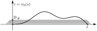
Figure 1. The initial data

Since the initial metric $g_{0}$ is singular at the north pole, the standard short-time existence theory for Ricci flow does not provide a solution. Because our initial metric is of the form (2.2) with $\psi_{0}(s)\sim s|\log s|^{-1/2}$ for $s\to 0$, the volume of a ball with radius $s$ centered at the singular point is $(C+o(1))s^{n+1}|\log s|^{-n/2}=o(s^{n+1})$. So no continuous metric $\tilde{g}$ on $\mathcal{S}^{n+1}$ exists for which $\exists c>0:c\tilde{g}\leq g_{\mathrm{can}}\leq c^{-1}\tilde{g}$. Therefore, neither the methods of Simon [27] nor of Koch–Lamm [19] can be used here to construct a solution.

Instead, we will construct a solution by regularizing the metric in a small neighborhood of the north pole, yielding a smooth metric $g_{\omega}$ for each small $\omega>0$, with $g_{\omega}\to g_{0}$ as $\omega\searrow 0$. Each of these may be regarded as a “surgically modified” solution, obtained by replacing the singularity with a smooth $(n+1)$-ball. The short-time existence theorem then guarantees the existence of a solution $g_{\omega}(t)$ on some time interval $0<t<T_{\omega}$, with $g_{\omega}$ as initial data. We will obtain a lower bound $T>0$ for $T_{\omega}$ and show that a subsequence of the $g_{\omega}$ converges in $C^{\infty}$ for all $0<t<T$.

The lower bound for $T_{\omega}$ follows easily from our previous characterization of singular solutions in [1]. Obtaining compactness of the solutions thus obtained turns out to be harder and will consume most of our efforts in Section 6.

In the following description of the regularized initial metric $g_{\omega}$, we will have to refer to a number of constants and functions which are properly defined in Sections 4 and 5. We note that while we have phrased the description in terms of the geometrically defined quantities $s,\psi,\psi_{s}$, it applies to metrics of the form (2.1).

For given small $\omega>0$, we split the manifold $\mathcal{S}^{n+1}$ into two disjoint parts, one of which is the small neighborhood $\mathcal{N}_{\omega}$ of the north pole in which $\psi_{0}(s)<\rho_{*}\sqrt{\omega}$.

On $\mathcal{S}^{n+1}\setminus\mathcal{N}_{\omega}$, we let our regularized metric $g_{\omega}$ coincide with the original metric $g_{0}$. Within $\mathcal{N}_{\omega}$, we let $g_{\omega}$ be a metric of the form $g_{\omega}=(ds)^{2}+\psi_{\omega}(s)^{2}g_{\mathrm{can}}$, where $\psi_{\omega}$ is a monotone function, at least when $\psi_{\omega}(s)\leq\rho_{*}\sqrt{\omega}$. In $\mathcal{N}_{\omega}$, we can therefore choose $r=\psi_{\omega}(s)$ as coordinate. In this coordinate, we require $g_{\omega}$ to be of the form

(2.3) $$g_{\omega}=\frac{(dr)^{2}}{v_{\omega}(r)}+r^{2}g_{\mathrm{can}},$$

where $v_{\omega}(r)$ satisfies

(2.4) $$v^{-}(r,\omega)\leq v_{\omega}(r)\leq v^{+}(r,\omega).$$

Here $v^{\pm}(\cdot,\omega)$ are the sub- and super- solutions constructed in Section 5, and evaluated at time $t=\omega$.

Recall that the scale-invariant difference of sectional curvatures,

$$a\doteqdot(L-K)\psi^{2}\quad\left(=\psi\psi_{ss}-\psi_{s}^{2}+1\right)$$

is uniformly bounded from above and below under Ricci flow [1, Corollary 3.2]. After possibly increasing the constant $\mathcal{A}$, we may assume that our regularized metrics $g_{\omega}$ satisfy hypotheses (M1)–(M8) in Table 1, with the exception that near $s=0$ one has $\psi_{\omega}^{\prime}(s)\to+1$ instead of (M4) and (M5) . Also, because we have modified the metric $g_{0}$ near the north pole, the distance $\ell_{\omega}$ between north and south poles will not be exactly $\ell$, although we do have $\ell_{\omega}=\ell+o(1)$ as $\omega\searrow 0$.

Solving Ricci flow starting from $g_{\omega}$ produces a family of metrics

$$g_{\omega}(t)=\varphi(x,t)^{2}(dx)^{2}+\psi(x,t)^{2}g_{\mathrm{can}}$$

which evolve according to (A.3). For these metrics, one will then have both

$$|\psi_{s}|\leq 1$$

and

$$|a_{\omega}|=|\psi\psi_{ss}-\psi_{s}^{2}+1|\leq\mathcal{A}.$$

Therefore, again by (A.3),

(2.5) $$|(\psi^{2})_{t}|=|2a+2n(\psi_{s}^{2}-1)|\leq 2(\mathcal{A}+n)$$

is bounded. In particular, one has $(\psi^{2})_{t}<2(\mathcal{A}+n)$ at critical points of $x\mapsto\psi(x,t)$. Thus if one sets

$$T_{0}=\frac{r_{\#}^{2}}{\mathcal{A}+n},$$

then condition (M7) implies that for $0<t<T_{0}$, the function $x\mapsto\psi(x,t)$ has no critical points with $\psi(x,t)\leq{r_{\#}}$. In particular, there can be no new neckpinch before $t=T_{0}$. We have thus proved

Lemma 1.

$\displaystyle T_{\omega}\geq T_{0}$ for all $\omega>0$.

Since $s\mapsto\psi_{\omega}(s,t)$ is monotone when $\psi_{\omega}<r_{\#}$, a function $r\mapsto u(r,t)$ is defined for $0<r<r_{\#}$ for which one has

(2.6) $$\psi_{s}(x,t)=u(r,t)=u\bigl{(}\psi(x,t),t\bigr{)}$$

for all $x$ on the northern cap of the sphere where $\psi\leq{r_{\#}}$ holds. With respect to these local coordinates, one may write the metric (2.2) as

$$g=\frac{(dr)^{2}}{u(r)^{2}}+r^{2}g_{\mathrm{can}}.$$

The sectional curvatures $K$ and $L$ defined in (A.2) are computed in these coordinates by $K=-uu_{r}/r$ and $L=(1-u^{2})/r^{2}$.

2.2. Evolution equations for $u(r,t)$ and $v(r,t)=u(r,t)^{2}$

To derive a differential equation for $u$, we first recall that $\psi_{s}$ satisfies

$$\partial_{t}\psi_{s}=\psi_{sss}+(n-2)\frac{\psi_{s}}{\psi}\psi_{ss}+(n-1)\frac{\psi_{s}(1-\psi_{s}^{2})}{\psi^{2}}.$$

On the other hand, from the definition (2.6) of $u$, we find by the chain rule that

$$\partial_{t}\psi_{s}=\psi_{t}u_{r}+u_{t}.$$

Combining these two relations, we get $u_{t}=\partial_{t}\psi_{s}-\psi_{r}u_{r}$ in terms of $\psi$ and its $s$ derivatives. To rewrite this in terms of $u$ and its derivatives, we use the fact that when $t$ is fixed, it follows from $u=\psi_{s}$ that

$$\frac{\partial}{\partial s}=u\frac{\partial}{\partial r},\quad\text{ and hence}\quad\psi_{ss}=uu_{r},\quad\psi_{sss}=u\bigl{(}uu_{r}\bigr{)}_{r}.$$

One then arrives at a parabolic pde for $u$, to wit,

(2.7) $$u_{t}=u\bigl{(}uu_{r}\bigr{)}_{r}-uu_{r}^{2}+\frac{n-1-u^{2}}{r}u_{r}+(n-1)\frac{u(1-u^{2})}{r^{2}}.$$

The quantity $v=u^{2}$ satisfies a similar but slightly simpler equation,

(2.8) $$v_{t}=\mathcal{F}[v],$$

where

(2.9) $$\mathcal{F}[v]\doteqdot vv_{rr}-\tfrac{1}{2}v_{r}^{2}+\frac{n-1-v}{r}v_{r}+\frac{2(n-1)}{r^{2}}v(1-v).$$

In terms of $v$, we have

(2.10) $$K=-\frac{v_{r}}{2r},\qquad L=\frac{1-v}{r^{2}}.$$

2.3. The shape of the singular initial data in the $r$ variables

We now derive the asymptotic behavior of the unmodified function $v(r,t)$ as $r\searrow 0$ at time $t=0$. First we estimate $u_{\mathrm{init}}(r)=u(r,0)$. By equation (A.4) of Lemma 14 in Appendix A, the quantity $r(s)=\psi(s,0)$ satisfies

(2.11) $$r=\left[\tfrac{1}{2}\sqrt{n-1}+o(1)\right]\frac{s}{\sqrt{-\log{s}}}$$

as the arc-length variable $s\searrow 0$. If this were an exact equation, one could solve it explicitly for $s$, yielding

$$s=r\sqrt{\frac{2}{n-1}\;W\left(\frac{n-1}{2r^{2}}\right)},$$

where $W$ denotes the Lambert-W (product-log) function, i.e. the inverse of $y\mapsto ye^{y}$ restricted to $(0,\infty)$. For our purposes, it suffices to notice that (2.11) implies that $\log r=\left[1+o(1)\right]\log s$ as $s\searrow 0$, hence that

(2.12) $$s=\left[\frac{2}{\sqrt{n-1}}+o(1)\right]r\sqrt{-\log r}$$

as $r\searrow 0$. Again by Lemma 14, it is permissible to differentiate (2.11), whereupon one finds in equation (A.5) that the initial data $u_{\mathrm{init}}(\cdot)=\psi_{s}(\cdot,0)$ satisfies

(2.13) $$u_{\mathrm{init}}(r)=\bigl{[}\frac{\sqrt{n-1}}{2}+o(1)\bigr{]}\frac{1}{\sqrt{-\log r}}$$

as $r\searrow 0$. Squaring, we conclude that $v$ initially must satisfy

(2.14) $$v_{\mathrm{init}}(r)=\bigl{(}\frac{n-1}{4}+o(1)\bigr{)}\frac{1}{-\log r}\quad(r\searrow 0).$$

3. Possible complete smooth solutions

In this paper, we construct smooth solutions $g(t)$ of Ricci flow on the compact sphere $\mathcal{S}^{n+1}$. However, our initial data are only smooth on the punctured sphere $\mathcal{S}^{n+1}\setminus\{\mathrm{NP}\}$. Inspired by Topping’s example in [31], one could also look for solutions on the punctured sphere which at all positive times $t$ represent complete metrics. Such solutions must necessarily be unbounded. Below, we will show that such solutions do not exist for our initial metric. Consequently, all possible smooth solutions starting from our singular initial metric extend to the compact sphere. Their sectional curvatures $K$ and $L$ must be bounded; and in view of $L=(1-v)/r^{2}$, we find that the quantity $v(r,t)$ must satisfy

(3.1) $$|v(r,t)-1|\leq\sup|L_{g(t)}|\;r^{2}.$$

Thus

(3.2) $$v(0,t)=1$$

is the only relevant boundary condition at $r=0$ for our problem.

Our existence proof of a solution starting from the singular initial metric involves the construction of a family of sub- and super- solutions $v^{\pm}_{\varepsilon,\delta}$, indexed by parameters $\varepsilon,\delta>0$. In this section, we show that the $v$ function corresponding to any smooth solution must lie between the sub- and super- solutions $v^{\pm}_{\varepsilon,\delta}$ to be constructed in Section 5.

3.1. Lower barriers for $v$

We first show that any such solution remains positive for small $r$ and $t$, with an estimate that proves the following result.

Theorem 2.

Any smooth complete rotationally symmetric forward Ricci flow evolution from a rotationally symmetric neckpinch singularity is compact with $v(0,t)=1$ for all $t>0$ that it exists.

Given $\lambda\in(0,1)$, define $\bar{v}_{\lambda}(r)$ for $0\leq r<1$ by $\bar{v}_{\lambda}(0)=0$ and

(3.3) $$\bar{v}_{\lambda}(r)\doteqdot\frac{\lambda(n-1)}{4}\frac{1}{-\log r}\qquad(0<r<1).$$

For later use, we note that for $r\in(0,1)$, one has

(3.4) $$(\bar{v}_{\lambda})_{r}=\frac{\lambda(n-1)}{4}\frac{1}{r(\log r)^{2}},$$

(3.5) $$(\bar{v}_{\lambda})_{rr}=\frac{\lambda(n-1)}{4}\left\{\frac{2}{r^{2}(-\log r)^{3}}-\frac{1}{r^{2}(\log r)^{2}}\right\}.$$

Theorem 2 is essentially a corollary of the following observation, which shows that on a sufficiently short time interval, $\bar{v}_{\lambda}(r)-\varepsilon(1+t)$ is a subsolution of (2.8) for all small $\varepsilon>0$.

Lemma 2.

Let $v$ be any nonnegative smooth function satisfying

(3.6) $$v_{t}\geq\mathcal{F}[v],\qquad v(r,0)\geq v_{\mathrm{init}}(r),$$

where $\mathcal{F}$ is defined by (2.9), and $v_{\mathrm{init}}$ satisfies (2.14).

Then $v\geq\bar{v}_{\lambda}$ on $(0,r_{0}]\times[0,t_{0}]$ for some small positive $r_{0}$ and $t_{0}$, independent of the boundary condition $v(0,\cdot)$.

We note that the following argument also allows $v$ to be a piecewise smooth supersolution whose graph only has concave corners, such as the “glued” supersolutions we construct in Section 5. We will only write the proof for the smooth case.

Proof.

Since $\lambda<1$, we may fix $0<r_{0}\ll 1$ so small that $\bar{v}_{\lambda}(r)<\min\left\{v_{\mathrm{init}}(r),\frac{1}{4}\right\}$ and $(\log r)^{2}>(n-1)/4$ for $0<r<r_{0}$. Then fix $t_{0}>0$ small enough so that $v(r,t)$ exists for $0<t\leq t_{0}$. By making $t_{0}$ smaller if necessary, we may assume that $\bar{v}_{\lambda}(r_{0})<v(r_{0},t)$ for $0\leq t\leq t_{0}$.

Given $\varepsilon>0$, define

(3.7) $$f_{\varepsilon}(r,t)\doteqdot v(r,t)-\bar{v}_{\lambda}(r)+\varepsilon(1+t).$$

We shall prove that $f_{\varepsilon}(r,t)>0$ for $0<r\leq r_{0}$. The lemma will follow by letting $\varepsilon$ go to zero.

To simplify the notation, we henceforth write $f\equiv f_{\varepsilon}$ and $\bar{v}\equiv\bar{v}_{\lambda}$. We also set $\mu\doteqdot\lambda(n-1)/4$.

Observe that $f(r,0)\geq\varepsilon$ for $0<r\leq r_{0}$ and that both $f(0,t)\geq\varepsilon$ and $f(r_{0},t)\geq\varepsilon$ hold for $0<t\leq t_{0}$. To obtain a contradiction, suppose that there exists a first time $\bar{t}\in(0,t_{0}]$ and a point $\bar{r}\in(0,r_{0}]$ such that $f(\bar{r},\bar{t})=0$. Then by (3.6), one has

(3.8) $$0\geq f_{t}(\bar{r},\bar{t})=\mathcal{F}\left[v(\bar{r},\bar{t})\right]+\varepsilon.$$

We claim that $\mathcal{F}\left[v(\bar{r},\bar{t})\right]\geq 0$. This contradicts (3.8) and proves the lemma.

To prove the claim, observe that

$$0=f_{r}(\bar{r},\bar{t})=v_{r}(\bar{r},\bar{t})-\bar{v}_{r}(\bar{r})\qquad\text{and}\qquad 0\leq f_{rr}(\bar{r},\bar{t})=v_{rr}(\bar{r},\bar{t})-\bar{v}_{rr}(\bar{r},\bar{t}).$$

Thus we obtain

$$\bar{r}^{2}\mathcal{F}\left[v(\bar{r},\bar{t})\right] =v\bar{r}^{2}v_{rr}-\frac{1}{2}(\bar{r}v_{r})^{2}+(n-1-v)\bar{r}v_{r}+2(n-1)(1-v)v$$

$$\geq v\bar{r}^{2}\bar{v}_{rr}-\frac{1}{2}(\bar{r}\bar{v}_{r})^{2}+(n-1-v)\bar{r}\bar{v}_{r}+2(n-1)(1-v)v$$

$$=\frac{\mu}{(\log r)^{2}}\left\{n-1-2v-\frac{\mu}{2(\log r)^{2}}\right\}$$

$$\hskip 86.11084pt+2v\left\{(n-1)(1-v)+\frac{\mu}{(-\log r)^{3}}\right\}$$

$$\geq\frac{\mu}{2(\log r)^{2}}\left\{1-\frac{\mu}{(\log r)^{2}}\right\}$$

$$>0.$$

Here we used the facts that $n\geq 2$ and $0\leq v<\bar{v}\leq 1/4$ at $(\bar{r},\bar{t})$. This proves the claim and hence the lemma. ∎

Now we can prove the main result of this subsection.

Proof of Theorem 2.

Let $\mathcal{K}_{r_{0}}$ denote the complement in $\mathcal{S}^{n+1}$ of the neighborhood of the north pole $\mathrm{NP}\in\mathcal{S}^{n+1}$ in which $\psi_{\mathrm{init}}<r_{0}$. For a smooth forward evolution, $\mathcal{K}_{r_{0}}$ is precompact for small positive time. So the only way a noncompact solution could develop is if a neighborhood of the singularity immediately became infinitely long. But for all $r\in(0,r_{0}]$, Lemma 2 implies that

$$\frac{1}{\sqrt{v(r,t)}}\leq\frac{2}{\sqrt{n-1}}\sqrt{-\log r}.$$

It follows that

$$d_{g(t)}(0,r_{0})=\int_{0}^{r_{0}}\frac{\,dr\,}{\sqrt{v(r,t)}}<\infty,$$

hence that the solution is compact. Because the sectional curvature of the metric $g$ on planes tangent to $\{r\}\times\mathcal{S}^{n}$ is $L=(1-v)/r^{2}$, the solution will be smooth only if $v(0,t)=1$. ∎

3.2. Yet another maximum principle

In this section, we prove that the $v$ function for any smooth, complete forward evolution with $g_{0}$ as initial metric is trapped between the sub- and super- solutions which we will construct in Section 5. This implies the claims about the asymptotic profile of the solution in Theorem 1.

We begin by establishing a suitable comparison principle.

Lemma 3.

Let $v^{-}$ and $v^{+}$ be nonnegative sub- and super- solutions, respectively, of $v_{t}=\mathcal{F}[v]$. Assume that either $v^{-}$ or $v^{+}$ satisfies

(3.9) $$v_{rr}\leq C,\quad K=-\frac{v_{r}}{2r}\leq C,\quad L=\frac{1-v}{r^{2}}\leq C$$

for some constant $C<\infty$ on a compact space-time set $\Xi=[0,\bar{r}]\times[0,\bar{t}]$.

If $v^{-}(\bar{r},t)\leq v^{+}(\bar{r},t)$ holds for $0\leq t\leq\bar{t}$, and $v^{-}(r,0)\leq v^{+}(r,0)$ holds for $0\leq r\leq\bar{r}$, then $v^{-}\leq v^{+}$ throughout $\Xi$.

In this lemma we assume that $v^{\pm}$ are smooth sub- and super- solutions. However, the proof works without modifications in the case where $v^{\pm}$ are piecewise smooth, where the graph of $v^{-}$ only has convex corners, and the graph of $v^{+}$ only has concave corners. In our maximum principle arguments, we shall only evaluate $v^{\pm}$ at “points of first contact with a given smooth solution” which are necessarily smooth points of $v^{\pm}$. Thus the hypothesis (3.9) is to be satisfied at all smooth points of $v^{+}$ or $v^{-}$; and, in particular, we do not intend to interpret the second derivative $v_{rr}$ in (3.9) in the sense of distributions.

Proof.

We prove the Lemma assuming that $v^{+}$ satisfies (3.9).

For $\lambda>0$ to be chosen later and any $\alpha>0$, define

(3.10) $$z=e^{-\lambda t}(v^{+}-v^{-})+\alpha.$$

Then $z>0$ on the parabolic boundary of $\Xi$. We shall prove that $z>0$ in $\Xi$. Because this implies that $v^{+}-v^{-}>-\alpha e^{\lambda\bar{t}}$ in $\Xi$, the lemma follows by letting $\alpha\searrow 0$.

Suppose there exists a first time $t\in(0,\bar{t}]$ and a point $r\in(0,\bar{r})$ such that $z(r,t)=0$. Then $z_{t}(r,t)\leq 0$, and

$$v^{+}(r,t)=v^{-}(r,t)-\alpha e^{\lambda t},\quad v^{+}_{r}(r,t)=v^{-}_{r}(r,t),\quad v^{+}_{rr}(r,t)\geq v^{-}_{rr}(r,t).$$

Hence at $(r,t)$, one has $0\geq e^{\lambda t}z_{t}$, where

$$e^{\lambda t}z_{t} =v^{+}_{t}-v^{-}_{t}-\lambda(v^{+}-v^{-})$$

$$=v^{-}[v^{+}_{rr}-v^{-}_{rr}]+(v^{-}-v^{+})\left\{\lambda-v^{+}_{rr}+\frac{v^{+}_{r}}{r}-2(n-1)\frac{1-v^{+}-v^{-}}{r^{2}}\right\}$$

$$\geq(v^{-}-v^{+})\left\{\lambda-v^{+}_{rr}+\frac{v^{+}_{r}}{r}-2(n-1)\frac{1-v^{+}-v^{-}}{r^{2}}\right\}.$$

Thus using the uniform bounds $v^{+}_{rr}\leq C$, $-v^{+}_{r}/r\leq C$, and $(1-v^{+})/r^{2}\leq C$ on $\Xi$, together with $v^{-}\geq 0$, one obtains

$$0\geq e^{\lambda t}z_{t}>\alpha e^{\lambda t}(\lambda-C).$$

This is a contradiction for any $\lambda>C$. The result follows.

To prove the Lemma in the case that the subsolution $v^{-}$ satisfies (3.9) one uses the fact that at a first zero $(r,t)$ of $z$ one has

$$e^{\lambda t}z_{t}=v^{+}[v^{+}_{rr}-v^{-}_{rr}]+(v^{-}-v^{+})\left\{\lambda-v^{-}_{rr}+\frac{v^{-}_{r}}{r}-2(n-1)\frac{1-v^{+}-v^{-}}{r^{2}}\right\}.$$

∎

Note that a different formulation of the lemma above is: if $v^{+}$ is a supersolution of $v_{t}=\mathcal{F}[v]$, then $v^{+}+\alpha e^{\lambda t}$ is a strict supersolution.

Theorem 3.

Let $v$ denote any solution of the Cauchy problem

$$v_{t}=\mathcal{F}[v],\qquad v(r,0)=v_{\mathrm{init}}(r),$$

that is smooth for a short time $0<t<t_{1}$. Let $v^{\pm}_{\varepsilon,\delta}$ denote the sub- and super- solutions, depending on $\varepsilon,\delta>0$, that are constructed in Section 5.

For all small enough $\varepsilon,\delta>0$, there exist $\bar{r}_{\varepsilon,\delta},\bar{t}_{\varepsilon,\delta}>0$ such that

(3.11) $$v^{-}_{\varepsilon,\delta}(r,t)\leq v(r,t)\leq v^{+}_{\varepsilon,\delta}(r,t)$$

for all $(r,t)\in\Xi=[0,\bar{r}]\times[0,\bar{t}]$.

Proof.

Let $\varepsilon,\delta>0$ be given.

Since $v$ assumes our initial data, we have $v(r,0)=(1+o(1))v_{0}(r)$ ($r\searrow 0$). Since the sub- and super- solutions are initially given by $v^{\pm}_{\varepsilon,\delta}(r,0)=(1\pm\delta)v_{0}(r)$, we find that there is some $\bar{r}>0$ such that $v^{-}_{\varepsilon,\delta}(r,0)<v(r,0)<v^{+}_{\varepsilon,\delta}(r,0)$ for all $r\in(0,\bar{r}]$.

The solution $v$ and the sub- and super- solutions $v^{\pm}_{\varepsilon,\delta}$ are smooth for $r>0$, so there is some $\bar{t}>0$ for which $v^{-}_{\varepsilon,\delta}(\bar{r},t)<v(\bar{r},t)<v^{+}_{\varepsilon,\delta}(\bar{r},t)$ holds for $0\leq t\leq\bar{t}$. After shrinking $\bar{t}$ if needed, we may also assume that $(1-\delta)v_{0}(\bar{r})<v(r,t)<(1+\delta)v_{0}(\bar{r})$ holds for $0\leq t\leq\bar{t}$.

Lemma 3 would now immediately provide us with the desired conclusion, but unfortunately neither $v$ nor $v^{\pm}_{\varepsilon,\delta}$ meet the requirements needed to apply that result. We overcome this problem by comparing time translates of $v$ and $v^{\pm}_{\varepsilon,\delta}$.

First we show that $v\geq v^{-}_{\varepsilon,\delta}$. Translate the given solution in time by a small amount $\kappa>0$, i.e. consider the function

$$\tilde{v}(r,t)=v(r,t+\kappa)$$

on the space-time domain $\Xi_{\kappa}=(0,\bar{r})\times(0,\bar{t}-\kappa)$. By Lemma 2, we know that $v(r,t)\geq v^{-}_{\varepsilon,\delta}(\bar{r},t)\geq(1-\delta)v_{0}(r)$ for $0<t<\bar{t}$. Since the time-translate $\tilde{v}$ is smooth, it does satisfy (3.9), and we may conclude that $\tilde{v}(r,t)\geq v^{-}(r,t)$ on $\Xi_{\kappa}$. Letting $\kappa\searrow 0$, we end up with $v(r,t)\geq v^{-}(r,t)$ on $\Xi$.

Next, we argue that $v\leq v^{+}_{\varepsilon,\delta}$ on $\Xi$. To this end we introduce

$$v^{*}(r,t)=v^{+}_{\varepsilon,\delta}(r,\kappa+t).$$

Since $v^{+}_{\varepsilon,\delta}$ is a supersolution that starts out with $v^{+}_{\varepsilon,\delta}(r,0)=(1+\delta)v_{0}(r)$, Lemma 2 tells us that $v^{+}_{\varepsilon,\delta}(r,t)\geq(1+\delta)v_{0}(r)>v(r,0)$ for all $(r,t)\in\Xi$. We already have $v^{+}_{\varepsilon,\delta}(\bar{r},t)>(1+\delta)v_{0}(\bar{r})>v(\bar{r},t)$ for $0<t\leq\bar{t}$. So, since $v^{*}$ is piecewise smooth and satisfies (3.9), we obtain $v(r,t)\leq v^{*}(r,t)$ on $\Xi_{\kappa}$. Letting $\kappa\searrow 0$ then completes the proof by showing that $v\leq v^{+}_{\varepsilon,\delta}$ on $\Xi$. ∎

4. Formal matched asymptotics

As a heuristic guide to what follows, we now construct an approximate solution of (2.8) that emerges from initial data satisfying $v(r,0)=v_{\mathrm{init}}(r)=[1+o(1)]v_{0}(r)$ as $r\searrow 0$, where by (2.14), $v_{0}$ is given by (1.4). By Theorem 2, we may restrict our attention to smooth solutions satisfying the (incompatible) boundary condition $v(0,t)=1$.

To describe the asymptotic behavior of the formal solution for small $t>0$, we split the $(r,t)$ plane into three regions, which we label inner, parabolic, and outer, as in the introduction.

We shall describe the solution in these separate but overlapping regions, working our way from the outer to the inner region.

4.1. The outer region $(r\sim 1)$

Away from $r=0$, we expect the solution to be smooth. So a good approximation of the solution at small $t>0$ should be

$$v(r,t)\approx v_{0}(r)+tv_{1}(r),$$

where $v_{1}\doteqdot\mathcal{F}[v_{0}]$. One computes that

$$\mathcal{F}[v_{0}] =\frac{v_{0}}{r^{2}}\left\{2(n-1)(1-v_{0})+\frac{1}{-\log r}\left((n-1)-2v_{0}+\frac{3v_{0}}{-2\log r}\right)\right\}$$

$$=\frac{v_{0}}{r^{2}}\left\{2(n-1)+\mathcal{O}\left(\frac{1}{-\log r}\right)\right\}.$$

So we set

(4.1) $$v_{\mathrm{out}}(r,t)\doteqdot{v}_{0}(r)\left[1+2(n-1)\frac{t}{r^{2}}\right]=\frac{n-1}{-4\log r}\left[1+2(n-1)\frac{t}{r^{2}}\right].$$

This suggests new space and time variables

(4.2) $$\rho=\frac{r}{\sqrt{t}},\qquad\tau=\log t.$$

With respect to $\rho$, which is bounded away from zero in the outer region, the outer approximation may be written in the form

(4.3) $$v_{\mathrm{out}}(r,t)=\frac{n-1}{-2\tau}\left[1+\frac{2(n-1)}{\rho^{2}}\right]+\mathcal{O}\bigl{(}\tau^{-2}\bigr{)}$$

as $t\searrow 0$, or, equivalently, as $\tau\searrow-\infty$.

4.2. The parabolic (intermediate) region $(r\sim\sqrt{t})$

With $\rho$ and $\tau$ given by (4.2), we define $W$ by

(4.4) $$v(r,t)=\frac{W(\rho,-\log t)}{-\log t}=\frac{W(\rho,\tau)}{-\tau}.$$

Then it is straightforward to compute that $W$ satisfies

(4.5) $$W_{\tau}+\frac{1}{-\tau}\bigl{\{}W-\mathcal{Q}_{\mathrm{par}}[W]\bigr{\}}=\mathcal{L}_{\mathrm{par}}[W],$$

where $\mathcal{L}_{\mathrm{par}}$ is the first-order linear operator

(4.6) $$\mathcal{L}_{\mathrm{par}}[W]\doteqdot\left(\frac{n-1}{\rho}+\frac{\rho}{2}\right)W_{\rho}+\frac{2(n-1)}{\rho^{2}}W,$$

and $\mathcal{Q}_{\mathrm{par}}$ is the quadratic form given by

(4.7) $$\mathcal{Q}_{\mathrm{par}}[W]\doteqdot WW_{\rho\rho}-\frac{1}{2}(W_{\rho})^{2}-\frac{1}{\rho}WW_{\rho}-\frac{2(n-1)}{\rho^{2}}W^{2}.$$

As $t\searrow 0$ one has $\tau=\log t\to-\infty$. So if the limit $\lim_{t\searrow 0}W(\rho,\tau)$ exists, equation (4.5) leads one to expect it to be a function $W_{0}(\rho)$ which satisfies $\mathcal{L}_{\mathrm{par}}[W_{0}]=0$. To get a better approximate solution, we can add correction terms of the form $W_{i}(\rho)/(-\tau)^{i}$ and substitute in (4.5). In this way one finds a formal asymptotic expansion of the form

(4.8) $$W(\rho,\tau)=W_{0}(\rho)+\frac{W_{1}(\rho)}{(-\tau)}+\frac{W_{2}(\rho)}{(-\tau)^{2}}+\cdots,$$

in which the $W_{j}$ can be computed inductively from

(4.9) $$\mathcal{L}_{\mathrm{par}}[W_{0}]=0,\quad\mathcal{L}_{{{\mathrm{par}}}}[W_{j+1}]=(j+1)W_{j}-\sum_{i=0}^{j}\mathcal{Q}_{\mathrm{par}}[W_{i},W_{j-i}].$$

Here $\mathcal{Q}_{\mathrm{par}}[\phi,\psi]$ is the bilinear form corresponding to the quadratic form $\mathcal{Q}_{\mathrm{par}}$ defined above.

We will not use this expansion beyond the lowest order term, but it did prompt us to look for the sub- and super- solutions which we find in Section 5.3.

Taking only the lowest order term, our approximate solution in the parabolic region is

(4.10) $$v_{\mathrm{par}}(r,t)=\frac{W_{0}(\rho)}{-\tau},$$

where $W_{0}$ is a solution of $\mathcal{L}_{\mathrm{par}}[W_{0}]=0$. The general solution of $\mathcal{L}_{\mathrm{par}}[W_{0}]=0$ is $W_{0}(\rho)=c_{0}[1+2(n-1)/\rho^{2}]$, which gives us

$$v_{\mathrm{par}}(r,t)=\frac{c_{0}}{-\tau}\left[1+\frac{2(n-1)}{\rho^{2}}\right].$$

Matching with (4.3) for fixed $\rho$ and $t\searrow 0$ tells us that the constant $c_{0}$ should be $c_{0}=(n-1)/2$. Thus we get

(4.11) $$W_{0}(\rho)=\frac{n-1}{2}\left[1+\frac{2(n-1)}{\rho^{2}}\right]$$

and

$$v_{\mathrm{par}}(r,t)=\frac{n-1}{-2\tau}\left[1+\frac{2(n-1)}{\rho^{2}}\right].$$

For small $\rho$, more precisely for $\rho=\mathcal{O}(1/\sqrt{-\tau})$, one defines a new space variable $\sigma=\rho\sqrt{-\tau}$ in order to write the approximation

(4.12) $$v_{\mathrm{par}}(r,t)\approx\frac{(n-1)^{2}}{\sigma^{2}}+\frac{n-1}{-2\tau}.$$

At first glance, it may be surprising that the approximate solution in the intermediate region is found by solving the first-order equation (4.6) rather than by finding a stationary solution of a parabolic equation. This is caused by the fact that the parabolic pde $v_{t}=\mathcal{F}[v]$ is degenerate when $v=0$.

If the solution $v$ were approximately self-similar with parabolic scaling, then one would have $v(\sqrt{t}\rho,t)\approx U(\rho)$ for some self-similarly-expanding solution $U$. However, equation (4.3) shows that this is incompatible with the behavior of $v$ near the “outer boundary” of the intermediate region.

Nonetheless, we remark that self-similarly-expanding Ricci solitons $U=\sqrt{V}$ do exist. These were first discovered by Bryant, in unpublished work. Each is a solution of the ode

(4.13) $$U^{2}U_{\rho\rho}+\left\{\frac{n-1-U^{2}}{\rho}+\frac{\rho}{2}\right\}U_{\rho}+\frac{n-1}{\rho^{2}}\left(1-U^{2}\right)U=0$$

derived from (2.7), but each emerges from initial data corresponding to a singular conical metric,

(4.14) $$g=\frac{(dr)^{2}}{U_{\infty}^{2}}+r^{2}g_{\mathrm{can}},$$

where $U_{\infty}>0$. We prove this assertion in Appendix B.

We shall see below that solutions to (4.13) with $U(0)=1$ and $U(\infty)=0$ do exist when the term $\frac{1}{2}\rho U^{\prime}$ in (4.13) is absent. These solutions correspond to the Bryant steady soliton.

Existence of solutions emerging from (4.14) also follows from Simon’s work [27], at least when $U_{\infty}$ is close to 1; but Simon does not require the hypothesis of $\textrm{SO}(n+1,\mathbb{R})$ symmetry.

4.3. The inner (slowly changing) region ($r\sim\sqrt{t/(-\log t)}$)

The formal solution in the parabolic scale $r=\mathcal{O}(\sqrt{T-t})$ found above becomes singular as $r\to 0$; and, in particular, it does not satisfy the boundary condition at $r=0$. Thus we look for a “boundary layer” at a smaller scale which will reconcile the incompatible initial $v(r,0)=0$ and boundary $v(0,t)=1$ $(t>0)$ conditions. Our derivation of the formal solution in the parabolic region suggests that the smaller length scale should be $\sqrt{t/(-\log t)}$. So we let

(4.15) $$\theta=\sqrt{\frac{t}{-\log t}},\qquad\sigma=\frac{r}{\theta}$$

and define

(4.16) $$v(r,t)=V\bigl{(}\sigma,\theta\bigr{)}.$$

Then $V$ satisfies the pde

(4.17) $$\theta\theta_{t}\bigl{\{}\theta V_{\theta}-\sigma V_{\sigma}\bigr{\}}=\mathcal{F}_{\mathrm{in}}[V],$$

where $\mathcal{F}_{{\mathrm{in}}}$ is obtained by replacing $r$-derivatives in $\mathcal{F}$ with $\sigma$-derivatives, namely

$$\mathcal{F}_{{\mathrm{in}}}[V]\doteqdot VV_{\sigma\sigma}-\tfrac{1}{2}(V_{\sigma})^{2}+\frac{n-1-V}{\sigma}V_{\sigma}+\frac{2(n-1)}{\sigma^{2}}(V-V^{2}).$$

We will abuse notation and simply write $\mathcal{F}$ for $\mathcal{F}_{\mathrm{in}}$.

We begin with the observation that $\theta\theta_{t}=\mathcal{O}\bigl{(}(-\log t)^{-1}\bigr{)}=o(1)$ for small $t$, so that the crudest approximation of (4.17) is simply the equation $\mathcal{F}[V]=0$. This ode admits a unique one-parameter family of complete solutions satisfying $V(0)=0$ and $V(\infty)=0$. These solutions are given by

$$V_{0}(\sigma)=\mathfrak{B}(k\sigma)\qquad(0<k<\infty),$$

where $\mathfrak{B}$ is the Bryant steady soliton, whose asymptotic behavior is $\mathfrak{B}(\sigma)=\sigma^{-2}+o(\sigma^{-2})$ for $\sigma\to\infty$. These assertions are proved in Appendix C.

Equation (4.17) suggests that this crude approximation is off by a term of order $\theta\theta_{t}$, which prompts us to look for approximate solutions of the form

(4.18) $$V(\sigma,t)=V_{0}(\sigma)+\theta\theta_{t}V_{1}(\sigma),$$

Here $V_{0}(\sigma)=\mathfrak{B}(k\sigma)$ contains an unspecified constant $k$ whose value we will determine later by matching with the approximate solution from the parabolic region.

To find an equation for $V_{1}$, we observe that the lhs and rhs of (4.17) applied to $V$ yield

(4.19) $$\theta\theta_{t}(\theta V_{\theta}-\sigma V_{\sigma})=-\theta\theta_{t}\sigma V_{0}^{\prime}(\sigma)+(\theta\theta_{t})^{2}\left[V_{1}(\sigma)-\sigma V_{1}^{\prime}(\sigma)\right]+\theta^{3}\theta_{tt}V_{1}(\sigma),$$

and

(4.20) $$\mathcal{F}[V_{0}+\theta\theta_{t}V_{1}]=\mathcal{F}[V_{0}]+d\mathcal{F}_{V_{0}}[\theta\theta_{t}V_{1}]+o(\theta\theta_{t}V_{1})=\theta\theta_{t}d\mathcal{F}_{V_{0}}[V_{1}]+o(\theta\theta_{t}V_{1}),$$

respectively. Here $d\mathcal{F}$ is the first variation of the nonlinear operator $\mathcal{F}$, defined by

$$d\mathcal{F}_{V}[W]=\left.\frac{d\mathcal{F}[V+\epsilon W]}{d\epsilon}\right|_{\epsilon=0}.$$

It is given by the ordinary differential operator

(4.21) $$d\mathcal{F}_{V_{0}}=V_{0}(\sigma)\frac{d^{2}}{d\sigma^{2}}+\left[\frac{n-1-V_{0}(\sigma)}{\sigma}-V_{0}^{\prime}(\sigma)\right]\frac{d}{d\sigma}\\ +\left[V_{0}^{\prime\prime}(\sigma)-\frac{V_{0}^{\prime}(\sigma)}{\sigma}+\frac{2(n-1)}{\sigma^{2}}(1-2V_{0}(\sigma))\right].$$

We note that

$$|\theta^{3}\theta_{tt}|+|\theta\theta_{t}|^{2}=o(\theta\theta_{t})\quad\text{as}\quad t\searrow 0.$$

So by keeping only the most significant terms in the lhs and rhs, we find the following equation for $V_{1}$,

(4.22) $$(d\mathcal{F}_{V_{0}})[V_{1}]=-\sigma V_{0}^{\prime}(\sigma).$$

We will first solve this equation in the case $k=1$ (when $V_{0}=\mathfrak{B}$). The general case then easily follows by rescaling.

Lemma 4.

The ordinary differential equation

$$d\mathcal{F}_{\mathfrak{B}}[\mathfrak{C}]=-\sigma\mathfrak{B}^{\prime}(\sigma)$$

has a strictly positive solution $\mathfrak{C}:(0,\infty)\to\mathbb{R}_{+}$ that satisfies

(4.23) $$\mathfrak{C}(\sigma)=\left\{\begin{array}[c]{cc}M\sigma^{2}+o(\sigma^{2})&(\sigma\searrow 0),\\ n-1+o(1)&(\sigma\nearrow\infty),\end{array}\right.$$

for some constant $M>0$.

All other solutions of $d\mathcal{F}_{\mathfrak{B}}[\mathfrak{C}]=-\sigma\mathfrak{B}^{\prime}(\sigma)$ that are bounded at $\sigma=0$ are given by ${\tilde{\mathfrak{C}}}(\sigma)=\mathfrak{C}(\sigma)-\lambda\sigma\mathfrak{C}^{\prime}(\sigma)$ for an arbitrary $\lambda\in\mathbb{R}$.

If $V_{0}(\sigma)=\mathfrak{B}(k\sigma)$ for any $k>0$, then

$$V_{1}(\sigma)=\frac{\mathfrak{C}(k\sigma)}{k^{2}}$$

is a solution of (4.22).

Proof.

We know that $\mathcal{F}[\mathfrak{B}(k\sigma)]=0$ for every $k>0$; differentiating this equation with respect to $k$ and setting $k=1$, we find that the homogeneous equation $d\mathcal{F}_{\mathfrak{B}}[\phi]=0$ has a solution

$$\phi(\sigma)\doteqdot-\sigma\mathfrak{B}^{\prime}(\sigma).$$

Given that $\phi$ satisfies $d\mathcal{F}_{\mathfrak{B}}[\phi]=0$, one can use the method of reduction of order to find a second (linearly independent) solution $\hat{\phi}$. One finds the following asymptotic behavior of $\hat{\phi}$ for small and large $\sigma$:

$$\hat{\phi}(\sigma)=\begin{cases}C\sigma^{-(n-1)}+o(\sigma^{-(n-1)})&(\sigma\searrow 0),\\ \exp\left\{-\sigma^{2}/2(n-1)+o(\sigma^{2})\right\}&(\sigma\nearrow\infty).\end{cases}$$

If $\mathfrak{C}_{p}$ is any particular solution of $d\mathcal{F}_{\mathfrak{B}}[\mathfrak{C}_{p}]=-\sigma\mathfrak{B}^{\prime}(\sigma)$, then the general solution to $d\mathcal{F}_{\mathfrak{B}}[\mathfrak{C}]=-\sigma\mathfrak{B}^{\prime}(\sigma)$ is

(4.24) $$\mathfrak{C}_{g}(\sigma)=a\phi(\sigma)+b\hat{\phi}(\sigma)+\mathfrak{C}_{p}(\sigma).$$

To obtain a particular solution which is bounded at $\sigma=0$, we note that for small $\sigma$, the equation $d\mathcal{F}_{\mathfrak{B}}[\mathfrak{C}]=-\sigma\mathfrak{B}^{\prime}$ is to leading order

$$\mathfrak{C}^{\prime\prime}+\frac{n-2}{\sigma}\mathfrak{C}^{\prime}-\frac{2(n-1)}{\sigma^{2}}\mathfrak{C}\approx-\mathfrak{B}^{\prime\prime}(0)\sigma^{2},$$

where $\mathfrak{B}^{\prime\prime}(0)<0$ by Lemma 18 in Appendix C. From this, one finds that a solution $\mathfrak{C}_{p}$ exists for which

(4.25) $$\mathfrak{C}_{p}(\sigma)=(K+o(1))\sigma^{4}\text{ as }\sigma\searrow 0,\text{ where }K=-\frac{\mathfrak{B}^{\prime\prime}(0)}{2(n+3)}>0.$$

Since $\hat{\phi}$ is not bounded at $\sigma=0$, the only solutions given in (4.24) which are bounded at $\sigma=0$ are those for which $b=0$.

Near $\sigma=\infty$, the equation $d\mathcal{F}_{\mathfrak{B}}[\mathfrak{C}]=-\sigma\mathfrak{B}^{\prime}$ is, to leading order,

$$\frac{1}{\sigma^{2}}\mathfrak{C}^{\prime\prime}+\frac{n-1}{\sigma}\mathfrak{C}^{\prime}+\frac{2(n-1)}{\sigma^{2}}\mathfrak{C}\approx\frac{2}{\sigma^{2}}.$$

One then finds that there also is a solution $\mathfrak{C}_{\infty}$, which satisfies

$$\mathfrak{C}_{\infty}(\sigma)=n-1+o(1)\qquad(\sigma\to\infty).$$

But $\mathfrak{C}_{\infty}(\sigma)-\mathfrak{C}_{p}(\sigma)$, being the difference of two particular solutions, is a linear combination of $\phi$ and $\hat{\phi}$. Since $\phi(\sigma)=o(1)$ and $\hat{\phi}(\sigma)=o(1)$ as $\sigma\to\infty$, we conclude that one also has

(4.26) $$\mathfrak{C}_{p}(\sigma)=n-1+o(1)$$

as $\sigma\to\infty$. So we see that the general solution of $d\mathcal{F}_{\mathfrak{B}}[\mathfrak{C}]=-\sigma\mathfrak{B}^{\prime}(\sigma)$ which is bounded as $\sigma\to 0$ is given by $\mathfrak{C}(\sigma)=\mathfrak{C}_{p}(\sigma)+a\phi(\sigma)$. Setting $a=-\lambda$ leads to the general solution described in the statement of the lemma.

The particular solution $\mathfrak{C}_{p}(\sigma)$ is positive for small and for large $\sigma$. The solution $-\phi(\sigma)=-\sigma\mathfrak{B}^{\prime}(\sigma)$ to the homogeneous equation is positive for all $\sigma>0$. Hence if one chooses $\lambda$ sufficiently large the resulting solution $\mathfrak{C}=\mathfrak{C}_{p}(\sigma)-\lambda\sigma\mathfrak{B}^{\prime}(\sigma)$ will be strictly positive for all $\sigma>0$. This is the positive solution of $d\mathcal{F}_{\mathfrak{B}}[\mathfrak{C}]=-\sigma\mathfrak{B}^{\prime}(\sigma)$ which was promised in the lemma.

Finally, if $d\mathcal{F}_{\mathfrak{B}}[\mathfrak{C}]=-\sigma\mathfrak{B}^{\prime}(\sigma)$ then one verifies by direct substitution that $V_{0}(\sigma)=\mathfrak{B}(k\sigma)$ and $V_{1}(\sigma)=k^{-2}\mathfrak{C}(k\sigma)$ satisfy (4.22). ∎

We return our attention to the approximate solution $V(\sigma,t)$ in (4.18). Combining $V_{0}(\sigma)=(1+o(1))(k\sigma)^{-2}$ and $V_{1}(\sigma)=n-1+o(1)$ for large $\sigma$ with the observation that

$$\theta\theta_{t}=\frac{1-\log t}{2(\log t)^{2}}=\frac{\frac{1}{2}+o(1)}{-\log t},\qquad(t\searrow 0),$$

one sees that for large $\sigma$ and small $t$ our approximate inner solution satisfies

$$V(\sigma,t)=V_{0}(\sigma)+\theta\theta_{t}V_{1}(\sigma)=[1+o(1)]\left\{\frac{1}{k^{2}\sigma^{2}}+\frac{1}{-2(n-1)k^{2}\log t}\right\}.$$

If we try to match this with the “small $\rho$ expansion” (4.12) for our approximate solution in the parabolic region, then we see that we should choose

(4.27) $$k=\frac{1}{n-1}.$$

5. Construction of the barriers

5.1. Outline of the construction

In this section, we will construct lower and upper barriers for the parabolic pde

$$v_{t}=\mathcal{F}[v]=\frac{1}{r^{2}}\left\{vr^{2}v_{rr}-\frac{1}{2}(rv_{r})^{2}+(n-1-v)rv_{r}+2(n-1)(1-v)v\right\}.$$

These barriers will apply to initial data satisfying

$$v_{\mathrm{init}}(r)=[1+o(1)]v_{0}(r)\quad\text{as}\quad r\searrow 0,$$

where $v_{0}$ is the asymptotic approximation defined in (1.4), namely

$$v_{0}(r)=\frac{n-1}{-4\log r}.$$

The barriers will be valid on a sufficiently small space-time region

$$0<r<r_{*},\qquad 0<t<t_{*}.$$

Note that $r_{*}$ will not exceed the quantity $r_{\#}$ from assumption (M7) concerning the initial metric. (See Section 2.1.)

Because we will not be able to write down barriers that are defined on this whole domain, our construction proceeds in two steps. Theorems 4, 5, and 6 constitute the first step. In this step, in accordance with the matched asymptotic description of the solution in Section 4, we will produce three sets of barriers, each in its own domain. (See Table 2.)

Outer	$\displaystyle(1\pm\delta)v_{0}(r)+(1\pm\varepsilon)t\mathcal{F}[(1\pm\delta)v_{0}(r)]$	$\displaystyle\rho_{*}\sqrt{t}\leq r\leq r_{*}$
Parabolic	$\displaystyle(1\pm\gamma_{\pm})\frac{W_{0}(\rho)}{-\tau}\pm\frac{B^{2}}{\tau^{2}\rho^{4}}$	$\displaystyle\frac{\sigma_{*}}{\sqrt{-\tau}}\leq\rho\leq 3\rho_{*}$
Inner	$\displaystyle\mathfrak{B}(k_{\pm}\sigma)+(1\mp\varepsilon)\theta\theta_{t}k_{\pm}^{2}\mathfrak{C}(k_{\pm}\sigma)$	$\displaystyle 0<\sigma\leq 3\sigma_{*}$

Table 2. The sub- and super- solutions with their domains. Here, $\delta$ and $\varepsilon$ are sufficiently small; $\rho_{*}=A\varepsilon^{-1/2}$, $\sigma_{*}=B\varepsilon^{-1/2}$ for certain constants $A,B$ depending only on $n$; and $\gamma_{\pm}$, $k_{\pm}$ are given by (5.2) and (5.3).

Note that the domains overlap. In all three cases, time is restricted to $0<t<t_{*}$. The parameters $r_{*}<r_{\#}$, $\rho_{*}$, $\sigma_{*}$, and $t_{*}$ will be defined during the construction. Although the construction admits free parameters $\gamma$, $\delta$, $\varepsilon$, and $k$, all but $\delta$ and $\varepsilon$ will be fixed in the second (“gluing”) step.

After constructing separate barriers, we must “glue” them together in order to make one pair of sub-/super- solutions. For example, to glue the subsolutions in the parabolic and outer regions, we define

$$v^{-}(r,t)=\begin{cases}v_{\mathrm{out}}^{-}(r,t)&3\rho_{*}\sqrt{t}\leq r\leq r_{*}\\ \mathstrut&\mathstrut\\ v_{\mathrm{par}}^{-}(r,t)&\sigma_{*}\sqrt{-t/\log t}\leq r\leq\rho_{*}\sqrt{t}\end{cases}$$

and

$$v^{-}(r,t)=\max\left\{v_{\mathrm{out}}^{-}(r,t),v_{\mathrm{par}}^{-}(r,t)\right\}$$

in the overlap between the outer and parabolic regions, when $\rho_{\ast}\sqrt{t}\leq r\leq 3\rho_{*}\sqrt{t}$. To be sure that this construction yields a true subsolution, we will verify the following “gluing condition”:

(5.1) $$v_{\mathrm{par}}(\rho_{*}\sqrt{t},t)>v_{\mathrm{out}}(\rho_{*}\sqrt{t},t)\text{ and }v_{\mathrm{par}}(3\rho_{*}\sqrt{t},t)<v_{\mathrm{out}}(3\rho_{*}\sqrt{t},t).$$

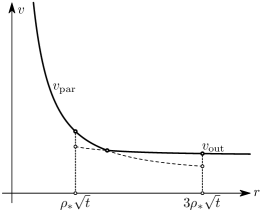
Figure 2. Gluing subsolutions

Lemmas 5 and 6 constitute the second step of the construction. When this step is completed, we will have chosen

(5.2) $$\gamma_{-}=\delta+\frac{(1-\delta)\varepsilon^{2}}{\varepsilon+2A^{2}/(n-1)}\quad\text{and}\quad k_{-}=\frac{1}{n-1}\,\frac{1}{\sqrt{1-\gamma_{-}-\varepsilon/2(n-1)^{2}}}$$

for subsolutions, and

(5.3) $$\gamma_{+}=\delta+\frac{(1+\delta)\varepsilon^{2}}{\varepsilon+2A^{2}/(n-1)}\quad\text{and}\quad k_{+}=\frac{1}{n-1}\,\frac{1}{\sqrt{1+\gamma_{+}-\varepsilon/2(n-1)^{2}}}$$

for supersolutions. Note that for small $\delta,\varepsilon>0$, one has $k_{-}>k_{+}$. Because $\mathfrak{B}(\sigma)$ is decreasing, this implies in particular that $V_{\mathrm{in}}^{-}<V_{\mathrm{in}}^{+}$ holds in the inner region.

5.2. Barriers in the outer region

In Section 4.1, we constructed an approximate solution of the form $v(r,t)=v_{0}(r)+tv_{1}(r)$. It turns out that a slight modification of this approximate solution yields both sub- and super- solutions in the outer region.

Theorem 4 (Outer Region).

There exist positive constants $A=A(n)$, $r_{*}=r_{*}(n)$, and $t_{*}=t_{*}(n,\varepsilon)$ such that for all $|\delta|\leq\frac{1}{2}$ and for all small $\varepsilon>0$, the functions

$$v_{\mathrm{out}}^{\pm}(r,t)=(1\pm\delta)v_{0}(r)+(1\pm\varepsilon)t\mathcal{F}[(1\pm\delta)v_{0}(r)]$$

are sub- $(v_{\mathrm{out}}^{-})$ and super- $(v_{\mathrm{out}}^{+})$ solutions in the region

$$\Omega_{\mathrm{out}}\doteqdot\left\{(r,t):\rho_{*}\sqrt{t}\leq r\leq r_{*},\quad 0<t<t_{*}\right\},$$

where $\rho_{*}=A/\sqrt{\varepsilon}$.

The constant $\delta$ need not be positive in this theorem, however, if one wants a properly ordered pair of sub- and super- solutions, i.e. if one wants $v_{\mathrm{out}}^{-}<v_{\mathrm{out}}^{+}$, then one must choose $\delta>0$.

Proof.

We will show that $v_{\mathrm{out}}^{-}$ is a subsolution in a domain $\rho_{*}\sqrt{t}\leq r\leq r_{*}$, where $r_{*}\leq r_{\#}$ and $\rho_{*}\gg 1$ are to be chosen. The proof that $v_{\mathrm{out}}^{+}$ is a supersolution is entirely analogous.

To simplify notation, we define constants

$$a\doteqdot(1-\delta)\tfrac{n-1}{4},\qquad b\doteqdot 1-\varepsilon,$$

and functions

$$\Lambda(r)\doteqdot\frac{1}{-\log r},\qquad\Gamma(r)\doteqdot\mathcal{F}\left[a\Lambda(r)\right].$$

We henceforth write $v_{\mathrm{out}}^{-}(r,t)$ as

(5.4) $$v_{a,b}(r,t)\doteqdot a\Lambda(r)+bt\Gamma(r).$$

Observe that

$$\Gamma(r)=\frac{a\Lambda}{r^{2}}\left\{2(n-1)+(n-1)(1-2a)\Lambda-2a\Lambda^{2}+\tfrac{3}{2}a\Lambda^{3}\right\}.$$

It follows that there exists $r_{*}>0$ such that

$$\Gamma(r)>C\frac{\Lambda}{r^{2}}\quad\text{for}\quad 0<r\leq r_{*}.$$

Because $\partial_{t}(v_{a,b})=b\Gamma$, we have

$$\partial_{t}(v_{a,b})-\mathcal{F}[v_{a,b}]=(b-1)\Gamma-\left\{\mathcal{F}[a\Lambda+bt\Gamma]-\mathcal{F}[a\Lambda]\right\}.$$

Here the first term $(b-1)\Gamma$ has a sign for $0<r<r_{*}$. The other term vanishes for $t=0$. So for small $t$, continuity of $\partial_{t}(v_{a,b})-\mathcal{F}[v_{a,b}]$ implies that $\partial_{t}(v_{a,b})-\mathcal{F}[v_{a,b}]<0$ if $b<1$. However, the size of the time interval on which this holds will depend on $r$ and, in particular, will shrink to zero as $r\to 0$. We now make this argument quantitative.

Using the splitting of $\mathcal{F}$ into linear and quadratic parts, one finds that

$$\mathcal{F}[a\Lambda+bt\Gamma]-\mathcal{F}[a\Lambda] =bt\mathcal{L}[\Gamma]+\mathcal{Q}(a\Lambda+bt\Gamma)-\mathcal{Q}(a\Lambda)$$

$$=bt\left\{\mathcal{L}[\Gamma]+\mathcal{Q}(2a\Lambda+bt\Gamma,\ \Gamma)\right\}$$

where the bilinear form $\mathcal{Q}(\cdot,\cdot)$ is defined by polarization from the quadratic form $\mathcal{Q}(\cdot)$, i.e. via

$$\mathcal{Q}(f,g)\doteqdot\tfrac{1}{4}\left\{Q(f+g)-Q(f-g)\right\}.$$

Both $\mathcal{L}[f]$ and $\mathcal{Q}(f,g)$ are conveniently estimated in terms of the pointwise semi-norm

$$[f]_{2}(r)\doteqdot\left|f(r)\right|+r\left|f_{r}(r)\right|+r^{2}\left|f_{rr}(r)\right|.$$

Indeed, for $0<r<r_{*}$,

$$\left|\mathcal{L}f\right|\leq\frac{C}{r^{2}}[f]_{2}\qquad\text{and}\qquad\left|\mathcal{Q}(f,g)\right|\leq\frac{C}{r^{2}}[f]_{2}[g]_{2}.$$

So for all $r<r_{*}$, one has

$$[a\Lambda]_{2}\leq C\Lambda\qquad\text{and}\qquad[\Gamma]_{2}\leq C\frac{\Lambda}{r^{2}}.$$

Therefore on the region $\rho_{*}\sqrt{t}\leq r\leq r_{*}$, one has

$$t[\Gamma]_{2}\leq\frac{C}{\rho_{*}^{2}}\Lambda.$$

For $\rho_{*}>1$, this implies that

$$\left|\mathcal{L}[\Gamma]+\mathcal{Q}(2a\Lambda+bt\Gamma,\ \Gamma)\right| \leq C\Lambda r^{-4}+C\Lambda^{2}r^{-4}+C\Lambda^{2}r^{-4}\rho_{*}^{-2}$$

$$\leq C\Lambda r^{-4}.$$

Observing that $\Gamma\geq C\Lambda r^{-2}$ for $0<r<r_{*}$, we thus estimate

$$t\left|\mathcal{L}[\Gamma]+\mathcal{Q}(2a\Lambda+bt\Gamma,\ \Gamma)\right|\leq\frac{C}{\rho_{*}^{2}}\frac{\Lambda}{r^{2}}\leq\frac{C}{\rho_{*}^{2}}\Gamma.$$

Returning to our estimate for $\partial_{t}(v_{a,b})-\mathcal{F}[v_{a,b}]$, we now have

$$\partial_{t}(v_{a,b})-\mathcal{F}[v_{a,b}]\leq(b-1)\Gamma+\frac{C}{\rho_{*}^{2}}\Gamma.$$

Because $\Gamma>0$, we may conclude that $v_{a,b}$ is a subsolution in the outer region $\rho_{*}\sqrt{t}\leq r\leq r_{*}$ provided that

$$\rho_{*}\geq C(1-b)^{-1/2}.$$

Because $1-b=\varepsilon>0$, the theorem follows by taking $A=C$. ∎

5.3. Barriers in the parabolic region

In the parabolic region, we use the similarity variables $\rho$, $\tau$, and $W$ defined in (4.2) and (4.4). According to (4.5) the function $W$ satisfies $\mathcal{D}_{\mathrm{par}}[W]=0$, where

$$\mathcal{D}_{\mathrm{par}}[W]\doteqdot W_{\tau}-\mathcal{L}_{\mathrm{par}}[W]+\frac{1}{-\tau}\{W-\mathcal{Q}_{\mathrm{par}}[W]\}.$$

Here $\mathcal{L}_{\mathrm{par}}$ is as in (4.6) while $\mathcal{Q}_{\mathrm{par}}[W]$ is the same quadratic differential polynomial as $\mathcal{Q}[v]$, but with all $r$-derivatives replaced by $\rho$-derivatives, namely

$$\mathcal{Q}_{\mathrm{par}}[W]\doteqdot\frac{1}{\rho^{2}}\bigl{\{}W\rho^{2}W_{\rho\rho}-\tfrac{1}{2}(\rho W_{\rho})^{2}-\rho W_{\rho}W-2(n-1)W^{2}\bigr{\}}.$$

Theorem 5 (Parabolic region).

Let $\varepsilon>0$, $\rho_{*}=A/\sqrt{\varepsilon}_{*}$ be as in Theorem 4.

There exist $B=B(n,\varepsilon)>1$, and $t_{*}=t_{*}(n,\varepsilon)$ such that for any $\gamma$ with $0\leq\gamma\leq\frac{1}{2}$, the functions

$$v_{\mathrm{par}}^{\pm}(r,t)\doteqdot\frac{W_{\mathrm{par}}^{\pm}(\rho,\tau)}{-\tau}$$

are sub- $(v_{\mathrm{par}}^{-})$ and super- $(v_{\mathrm{par}}^{+})$ solutions in the region

$$\Omega_{\mathrm{par}}\doteqdot\left\{(r,t):\frac{B}{\sqrt{\varepsilon}}\sqrt{\frac{t}{-\log t}}\leq r\leq 3\rho_{*}\sqrt{t},\quad 0<t<t_{\ast}\right\}.$$

Here

$$W_{\mathrm{par}}^{\pm}(\rho,\tau)\doteqdot(1\pm\gamma)W_{0}(\rho)\pm\frac{B^{2}}{-\tau\rho^{4}},$$

where $W_{0}(\rho)$ is as in (4.11).

Proof.

We consider the case of a subsolution. Recall that $cW_{0}$ is the general solution of the first-order ode $\mathcal{L}_{\mathrm{par}}[W]=0$. Moreover,

(5.5) $$\mathcal{L}_{\mathrm{par}}[\rho^{-4}]=-2\rho^{-6}(n-1+\rho^{2})\leq-2(n-1)\rho^{-6}.$$

To show that $W_{\mathrm{par}}^{-}$ is a subsolution, we will verify that $\mathcal{D}_{\mathrm{par}}[W_{\mathrm{par}}^{-}]<0$ on $\Omega_{\mathrm{par}}$. To simplify notation, we write $W\equiv W_{\mathrm{par}}^{-}$ for the remainder of the proof.

Observe that

$$[W]_{2}\doteqdot|W|+\rho|W_{\rho}|+\rho^{2}|W_{\rho\rho}|\leq C\left(\rho^{-2}+B^{2}|\tau|^{-1}\rho^{-4}\right)$$

if $\rho\leq 3\rho_{*}=3A/\sqrt{\varepsilon}$, where $C=C(n,A,\varepsilon)$. In the parabolic region $\Omega_{\mathrm{par}}$ defined above, one has

(5.6) $$0<\frac{B}{(-\tau)\rho^{2}}\leq\varepsilon,$$

whence we get

$$[W]_{2}\leq C\rho^{-2}$$

and also

$$|\mathcal{Q}_{\mathrm{par}}(W)|\leq\frac{C}{\rho^{2}}[W]_{2}^{2}\leq\frac{C^{\prime}}{\rho^{6}}.$$

Now we compute that

$$(-\tau)\mathcal{D}_{\mathrm{par}}[W]=-\frac{2B^{2}}{(-\tau)\rho^{4}}+B^{2}\mathcal{L}_{\mathrm{par}}[\rho^{-4}]+(1-\gamma)W_{0}-\mathcal{Q}_{\mathrm{par}}[W].$$

Assuming that $\tau\leq-1$, we find, using (5.5), (5.6), and also $\rho\leq 3\rho_{*}=3A/\sqrt{\varepsilon}$, that

$$(-\tau)\mathcal{D}_{\mathrm{par}}[W]\leq\frac{C-2(n-1)B^{2}}{\rho^{6}}$$

in the parabolic region. Hence we conclude that the function $W\equiv W_{\mathrm{par}}^{-}$ will indeed be a subsolution provided that $B^{2}\geq\max\{1,C/2(n-1)\}$.

The left- and right- end points of the parabolic region at any time $\tau$ are given by $\rho=B/\sqrt{\varepsilon(-\tau)}$ and $\rho=3\rho_{*}=3A/\sqrt{\varepsilon}$, respectively. So this region will be nonempty if $-\infty<\tau<-B^{2}/(3A)^{2}$. Thus we choose $\tau_{*}=-\max\left\{1,B^{2}/(3A)^{2}\right\}$.

Construction of supersolutions $W_{\mathrm{par}}^{+}$ is similar. ∎

5.4. Barriers in the inner region

In the inner region, we work with the space and time variables $\sigma$, $\theta$ defined in (4.15). We consider $V(\sigma,\theta)=v(r,t)$, as in (4.16). Then, according to (4.17), Ricci flow is equivalent to $\mathcal{D}_{\mathrm{in}}[V]=0$, where

$$\mathcal{D}_{\mathrm{in}}[V] \doteqdot\theta\theta_{t}\left(\theta V_{\theta}-\sigma V_{\sigma}\right)-\mathcal{F}[V]$$

$$=\theta^{2}V_{t}-\theta\theta_{t}\sigma V_{\sigma}-\mathcal{F}[V].$$

The formal solution we found in Section 4.3 is of the form

$$V(\sigma,t)=V_{0}(\sigma)+\lambda\theta\theta_{t}V_{1}(\sigma),$$

where

$$V_{0}(\sigma)=\mathfrak{B}(k\sigma),\text{ and }V_{1}(\sigma)=k^{-2}\mathfrak{C}(k\sigma).$$

In Section 4.3, we chose $\lambda=1$ and $k=1/(n-1)$ in order to match this solution with the formal solution in the parabolic region. Here we will show that small variations in $k$ and $\lambda$ lead to sub- and super- solutions.

Theorem 6 (Inner Region).

Let $\varepsilon$ and $B$ be as before. There exists $t_{*}=t_{*}(n,\varepsilon,B)$ such that for any $k\in[\frac{1}{2(n-1)},\frac{2}{n-1}]$, the functions

$$v_{\mathrm{in}}^{\pm}(r,t)=V_{\mathrm{in}}^{\pm}(\sigma,\theta)\doteqdot\mathfrak{B}(k\sigma)+(1\mp\varepsilon)\theta\theta_{t}k^{-2}\mathfrak{C}(k\sigma)$$

are sub- $(v_{\mathrm{in}}^{-})$ and super- $(v_{\mathrm{in}}^{+})$ solutions in the region

$$\Omega_{\mathrm{in}}\doteqdot\left\{(r,t):0<r\leq 3\frac{B}{\sqrt{\varepsilon}}\sqrt{\frac{t}{-\log t}},\quad 0<t<t_{*}\right\}.$$

We draw the reader’s attention to the fact that $\theta\theta_{t}\mathfrak{C}(k\sigma)>0$. So for fixed $k$, the subsolution $V_{{\mathrm{in}}}^{-}$ is larger than the formal solution (which has $\varepsilon=0$), while the supersolution $V_{\mathrm{in}}^{+}$ is smaller. To get a properly ordered pair of sub- and super- solutions, we must (and can) choose $V_{\mathrm{in}}^{+}$ and $V_{\mathrm{in}}^{-}$ with different values of $k$.

Proof.

We will prove that

$$V_{\mathrm{in}}^{-}=V_{0}(\sigma)+(1+\varepsilon)\theta\theta_{t}V_{1}(\sigma),\text{ with }V_{0}(\sigma)=\mathfrak{B}(k\sigma)\text{ and }V_{1}(\sigma)=k^{2}\mathfrak{C}(k\sigma),$$

is a subsolution in the region $\Omega_{\mathrm{in}}$, i.e. for

$$0<\sigma<3\sigma_{*}=3B/\sqrt{\varepsilon},\qquad 0<t<t_{*},$$

where $t_{*}$ is suitably chosen. The proof that $V_{\mathrm{in}}^{+}$ is a supersolution is similar.

Upon substitution, we find that

(5.7) $$\mathcal{D}_{\mathrm{in}}[V_{\mathrm{in}}^{-}]=\theta^{2}(1+\varepsilon)(\theta\theta_{t})_{t}V_{1}-\theta\theta_{t}\sigma V_{0}^{\prime}-(1+\varepsilon)(\theta\theta_{t})^{2}\sigma V_{1}^{\prime}-\mathcal{F}\bigl{[}V_{0}+(1+\varepsilon)\theta\theta_{t}V_{1}\bigr{]}.$$

We can expand the last term, keeping in mind that $\mathcal{F}[V_{0}]=0$, and that $\mathcal{F}[V]$ is a quadratic polynomial in $V$ and its derivatives. We get

$$\mathcal{F}\bigl{[}V_{0}+(1+\varepsilon)\theta\theta_{t}V_{1}\bigr{]}=(1+\varepsilon)\theta\theta_{t}d\mathcal{F}_{V_{0}}[V_{1}]+(1+\varepsilon)^{2}(\theta\theta_{t})^{2}\mathcal{Q}[V_{1}],$$

where

$$\mathcal{Q}[V]=VV_{\sigma\sigma}-\tfrac{1}{2}(V_{\sigma})^{2}-\tfrac{1}{\sigma}VV_{\sigma}-\tfrac{2(n-1)}{\sigma^{2}}V^{2}$$

is the quadratic part of $\mathcal{F}[V]$. Applying this expansion to (5.7), we find that

(5.8) $$\mathcal{D}_{\mathrm{in}}[V_{\mathrm{in}}^{-}]=\varepsilon\theta\theta_{t}\sigma V_{0}^{\prime}+(1+\varepsilon)\theta^{2}(\theta\theta_{t})_{t}V_{1}-(1+\varepsilon)(\theta\theta_{t})^{2}\sigma V_{1}^{\prime}-(1+\varepsilon)^{2}(\theta\theta_{t})^{2}\mathcal{Q}[V_{1}]$$

The key to our argument is that the first term dominates the others on the interval $0<\sigma<\sigma_{*}=3B/\sqrt{\varepsilon}$.

The facts from Lemma 18 that the Bryant soliton $\mathfrak{B}(\cdot)$ is strictly decreasing, and that it is given by $\mathfrak{B}(\sigma)=1+b_{2}\sigma^{2}+\cdots$ for small $\sigma$, with $b_{2}<0$, tell us that there is a constant $\eta>0$ such that

(5.9) $$-\sigma V_{0}^{\prime}(\sigma)\geq\eta\sigma^{2}\text{ for }\sigma\in(0,3\sigma_{*}).$$

The asymptotics of $\mathfrak{C}(\sigma)$ both at $\sigma=0$ and $\sigma=\infty$ from Lemma 4 tell us that for some $C=C(n,\mathfrak{C})<\infty$, one has

(5.10) $$|V_{1}|+|\sigma V_{1}^{\prime}|+|\mathcal{Q}[V_{1}]|\leq C\sigma^{2}\text{ for all }\sigma\in(0,3\sigma_{*}),$$

provided that $\sigma_{*}>1$. Finally, by direct computation, one finds that

$$\theta\theta_{t}=\tfrac{1}{2}\bigl{(}\frac{1}{-\log t}+\frac{1}{(-\log t)^{2}}\bigr{)},\qquad\theta^{2}(\theta\theta_{t})_{t}=\frac{1+\frac{2}{-\log t}}{2(-\log t)^{3}},$$

so that $|\theta^{2}(\theta\theta_{t})_{t}|\leq C(\theta\theta_{t})^{3}$ for some $C<\infty$, and for small $t$.

Together with (5.9) and (5.10), we find that

(5.11) $$\mathcal{D}[V_{\mathrm{in}}]\leq\left\{-\eta\varepsilon+C\theta\theta_{t}\right\}\theta\theta_{t}\sigma^{2}$$

for all $\sigma\in(0,3\sigma_{*})$. Since $\theta\theta_{t}=o(1)$ as $t\searrow 0$, we find that $V_{\mathrm{in}}^{-}$ is indeed a supersolution for small enough $t$. ∎

5.5. Gluing the outer and parabolic barriers

The barriers $W_{\mathrm{par}}^{\pm}$ constructed in Section 5.3 generate sub- and super- solutions

$$v_{\mathrm{par}}^{\pm}=\frac{W_{\mathrm{par}}^{\pm}}{-\log t}$$

for the original equation $v_{t}=\mathcal{F}[v]$ in the parabolic region.

Lemma 5.

Let $A,\epsilon$ and $\delta$ be as before, and set

(5.12) $$\gamma=\gamma_{-}(\delta,\varepsilon)=\delta+\frac{(1-\delta)\varepsilon^{2}}{\varepsilon+2A^{2}/(n-1)}.$$

If $-\tau_{*}$ is sufficiently large, then the gluing condition (5.1) is satisfied for all $\tau<\tau_{*}$.

Proof.

We will verify the relations

$$v_{\mathrm{par}}(\rho_{*}\sqrt{t},t)>v_{\mathrm{out}}(\rho_{*}\sqrt{t},t)\text{ and }v_{\mathrm{par}}(3\rho_{*}\sqrt{t},t)<v_{\mathrm{out}}(3\rho_{*}\sqrt{t},t)$$

in the $W(\rho,\tau)$ rather than the $v(r,t)$ notation.

When written in the $(\rho,\tau)$ variables, the subsolutions from the outer region take the form

$$W_{\mathrm{out}}^{-}(\rho,\tau)\ =(-\tau)a{\Lambda}\left\{1+(1-\varepsilon)\frac{2(n-1)+\mathcal{O}(\Lambda)}{\rho^{2}}\right\},$$

where

$$a\doteqdot(1-\delta)\frac{n-1}{4}.$$

If $\rho_{*}\leq\rho\leq 3\rho_{*}$, then

$$\Lambda=\frac{1}{-\log r}=\frac{1}{-\log\rho-\frac{1}{2}\log t}=-2\tau^{-1}+\mathcal{O}(\tau^{-2}).$$

Hence

$$W_{\mathrm{out}}^{-}(\rho,\tau)=(1-\delta)\frac{n-1}{2}\left\{1+\frac{2(n-1)(1-\varepsilon)}{\rho^{2}}\right\}+\mathcal{O}(\tau^{-1}),\quad(\tau\to-\infty),$$

uniformly in $\rho_{*}\leq\rho\leq 3\rho_{*}$.

The subsolutions from the parabolic region satisfy

$$W_{\mathrm{par}}^{-}(\rho,\tau)=(1-\gamma)\frac{n-1}{2}\left\{1+\frac{2(n-1)}{\rho^{2}}\right\}+\mathcal{O}(\tau^{-1}),\quad(\tau\to-\infty).$$

The outer and parabolic subsolutions have limits as $\tau\to-\infty$, namely

$$W_{\mathrm{out}}^{-\infty}(\rho) \doteqdot(1-\delta)\frac{n-1}{2}\left\{1+(1-\varepsilon)\frac{2(n-1)}{\rho^{2}}\right\},$$

$$W_{\mathrm{par}}^{-\infty}(\rho) \doteqdot(1-\gamma)\frac{n-1}{2}\left\{1+\frac{2(n-1)}{\rho^{2}}\right\},$$

respectively. At $\rho=0,\infty$, one finds that

(5.13) $$\frac{W_{\mathrm{out}}^{-\infty}(\rho)}{W_{\mathrm{par}}^{-\infty}(\rho)}\longrightarrow\begin{cases}\dfrac{1-\delta}{1-\gamma}&\text{ as $\rho\to\infty$,}\\ (1-\varepsilon)\dfrac{1-\delta}{1-\gamma}&\text{ as $\rho\to 0$.}\end{cases}$$

Requiring $W_{\mathrm{out}}^{-\infty}(2\rho_{*})=W_{{\mathrm{par}}}^{-\infty}(2\rho_{*})$ leads to (5.12). (Use $\rho_{*}=A/\sqrt{\varepsilon}$.) If (5.12) holds, then $\rho=2\rho_{*}$ is the only solution of $W_{\mathrm{out}}^{-\infty}(\rho)=W_{\mathrm{par}}^{-\infty}(\rho)$, and it follows from (5.13) that

$$W_{\mathrm{out}}^{-\infty}(\rho_{*})<W_{\mathrm{par}}^{-\infty}(\rho_{*})\text{ and }W_{\mathrm{out}}^{-\infty}(3\rho_{*})>W_{\mathrm{par}}^{-\infty}(3\rho_{*}).$$

In particular, the gluing condition (5.1) is met.

Because $W_{\mathrm{out}}^{-}$ and $W_{\mathrm{par}}^{-}$ are small ($\mathcal{O}(\tau^{-1})$) perturbations of $W_{\mathrm{out}}^{-\infty}\$ and $W_{\mathrm{par}}^{-\infty}$, respectively, these inequalities will continue to hold for all sufficiently large $-\tau$. ∎

A similar statement holds true for supersolutions.

5.6. Gluing the inner and parabolic barriers

Recall that the inner and parabolic regions are

$$\Omega_{\mathrm{in}} =\left\{0<\sigma\leq 3\sigma_{*},\quad 0<t<t_{*}\right\},$$

$$\Omega_{\mathrm{par}} =\left\{\sigma_{*}\leq\sigma\leq 3A\sqrt{-\tau}/\sqrt{\varepsilon},\quad 0<t<t_{*}\right\},$$

respectively, where

$$\sigma_{*}=B/\sqrt{\varepsilon}.$$

We now verify the “gluing condition” between the inner and parabolic regions.

Lemma 6.

If

(5.14) $$k=k_{-}(\delta,\varepsilon)=\frac{1}{n-1}\,\frac{1}{\sqrt{1-\gamma-\varepsilon/2(n-1)^{2}}}$$

and if $B$ is sufficiently large (depending only on $n$), then the gluing conditions

(5.15) $$V_{\mathrm{in}}^{-}(\sigma_{*},\tau)>V_{\mathrm{par}}^{-}(\sigma_{*},\tau)\text{ and }V_{\mathrm{in}}^{-}(3\sigma_{*},\tau)<V_{\mathrm{par}}^{-}(3\sigma_{*},\tau)$$

are satisfied for all $\tau<\tau_{*}$, provided that $-\tau_{*}$ is sufficiently large.

Proof.

By Theorem 6, the subsolutions in the inner region $\Omega_{\mathrm{in}}$ have a limit as $t\searrow 0$, equivalently, as $\tau\searrow-\infty$. The limit is

(5.16) $$V_{\mathrm{in}}^{-\infty}(\sigma)=\lim_{t\searrow 0}V_{\mathrm{in}}^{-}(\sigma,t)=\mathfrak{B}(k\sigma).$$

Our asymptotic expansion of the Bryant soliton (Lemma 18) implies that

(5.17) $$\mathfrak{B}(k\sigma)=(k\sigma)^{-2}+\mathcal{O}\left((k\sigma)^{-4}\right),\qquad(\sigma\to\infty).$$

By Theorem 5, the subsolutions in the parabolic region $\Omega_{\mathrm{par}}$ also have limits at $t=0,\tau=-\infty$, namely

(5.18) $$V_{\mathrm{par}}^{-\infty}(\sigma)=\lim_{t\searrow 0}v_{\mathrm{par}}^{-}(\sigma\theta,t)=\frac{(1-\gamma)(n-1)^{2}}{\sigma^{2}}-\frac{B^{2}}{\sigma^{4}}$$

Equations (5.16) and (5.18) show that to establish (5.15), it will suffice to prove

(5.19) $$V_{\mathrm{in}}^{-\infty}(\sigma_{*})>V_{\mathrm{par}}^{-\infty}(\sigma_{*})\text{ and }V_{\mathrm{in}}^{-\infty}(3\sigma_{*})<V_{\mathrm{par}}^{-\infty}(3\sigma_{*})$$

and then to choose $-\tau_{*}$ sufficiently large such that $V_{\mathrm{in}}^{-}(\sigma_{*},\tau)>V_{\mathrm{par}}^{-}(\sigma_{*},\tau)$ and $V_{\mathrm{in}}^{-}(3\sigma_{*},\tau)<V_{\mathrm{par}}^{-}(3\sigma_{*},\tau)$ are preserved for all $\tau<\tau_{*}$.

Without loss of generality, we may assume that $\frac{1}{2}(n-1)^{-1}<k<2(n-1)^{-1}$. Then by (5.17), there is a constant $C_{n}<\infty$ such that

(5.20) $$\left|\sigma^{2}V_{\mathrm{in}}^{-\infty}-k^{-2}\right|\leq C_{n}\sigma^{-2}$$

for all $\sigma\geq 1$ and all $k$ under consideration.

Hence we have

$$\sigma^{2}\left(V_{\mathrm{in}}^{-\infty}-V_{\mathrm{par}}^{-\infty}\right)=k^{-2}-(1-\gamma)(n-1)^{2}+(B^{2}+\vartheta C_{n})\sigma^{-2},$$

where $|\vartheta|\leq 1$. In order to verify (5.19), we must find the sign of the lhs for $\sigma=m\sigma_{*}$, with $m=1$ or $m=3$. Using $\sigma_{*}=B\varepsilon^{-1/2}$, we find that when $\sigma=m\sigma_{*}$,

$$\sigma^{2}\bigl{(}V_{\mathrm{in}}^{-\infty}-V_{\mathrm{par}}^{-\infty}\bigr{)}=k^{-2}-(1-\gamma)(n-1)^{2}+\frac{\varepsilon}{m^{2}}(1+\vartheta C_{n}B^{-2}).$$

In particular, (5.19) will hold if this quantity is positive for $m=1$ and negative for $m=3$. We can achieve this by first choosing $B$ so large that we can ignore the term containing $\vartheta$: $B\geq B_{n}\doteqdot\sqrt{100C_{n}}$ will do. Then we choose $k$ so as to satisfy

$$k^{-2}-(1-\gamma)(n-1)^{2}=-\frac{\varepsilon}{2}.$$

Solving this for $k$ leads to the value $k_{-}(\delta,\varepsilon)$ mentioned in the Lemma. Once $k$ is given this value and $B$ is chosen large enough, (5.19) will hold.

∎

A similar statement holds for supersolutions.

6. Subsequential convergence of the regularized solutions

In this section, we prove compactness of the family $\{g_{\omega}(t)\mid 0<t\leq T\}$ for some $0<T<T_{0}$. We find a convergent subsequence $g_{\omega_{j}}(t)\to g_{*}(t)$; we show that $g_{*}(t)$ is a smooth solution on $\mathcal{S}^{n+1}$ for small $t>0$; and we verify that $g_{*}(t)$ is indeed a forward evolution from the singular initial metric $g_{0}$.

We do this directly, rather than by invoking Hamilton’s compactness theorem, which instead gives $\eta_{j}^{*}(g_{\omega_{j}})(t)\to\tilde{g}_{*}(t)$ for some sequence $\{\eta_{j}:\mathcal{S}^{n+1}\to\mathcal{S}^{n+1}\}$ of time-independent diffeomorphisms fixing the north pole $\mathrm{NP}\in\mathcal{S}^{n+1}$ [14].

The main problem in establishing compactness is that, although we have precise control of the $v$ function near the singular point, this information is only valid in a neighborhood of the form $\{P\in\mathcal{S}^{n+1}\mid\psi(P,t)\leq\bar{r}\}$ for some $\bar{r}>0$.

6.1. Splitting $\mathcal{S}^{n+1}$ into regular and singular parts

The following lemma allows us to split the manifold $\mathcal{S}^{n+1}$ into a regular and a singular part.

Lemma 7 (Existence of collars).

For any $0<m<1$ and small enough $\alpha>0$, there exists $T=T(\alpha)\in(0,T_{0})$ such that for $0<t<T(\alpha)$, the function

$${v_{\mathrm{col}}}^{+}(r,t)=\min\left\{1,me^{3t/\alpha^{2}}+\left(\frac{r-\bar{r}}{\alpha}\right)^{2}\right\}$$

is a supersolution of $v_{t}=\mathcal{F}[v]$, while

$${v_{\mathrm{col}}}^{-}(r,t)=\max\left\{0,me^{-t/\alpha^{2}}-\left(\frac{r-\bar{r}}{\alpha}\right)^{2}\right\}$$

is a subsolution.

Proof.

The statements are verified by direct computation. For $G_{\pm}(z)=m\pm z^{2}$ one computes that

$$\mathcal{F}\left[G_{+}\left(\frac{r-\bar{r}}{\alpha}\right)\right]=\alpha^{-2}\left[2m+\mathcal{O}(\alpha)\right],$$

and

$$\mathcal{F}\left[G_{-}\left(\frac{r-\bar{r}}{\alpha}\right)\right]=\alpha^{-2}\left[2m-2\bigl{(}\frac{r-\bar{r}}{\alpha}\bigr{)}^{2}+\mathcal{O}(\alpha)\right],$$

hold when $|r-\bar{r}|\leq\alpha$, and when $\alpha\leq\tfrac{1}{2}\bar{r}$.

If we now let $m$ vary with time, we find that $m(t)-z^{2}$ is a subsolution for small $\alpha$ if $m^{\prime}(t)<cm(t)/\alpha^{2}$ for any constant $c<0$: we choose $c=-1$ to get the subsolution in the Lemma. Similarly, $m(t)+z^{2}$ is a supersolution if $m^{\prime}(t)>cm(t)/\alpha^{2}$ for any constant $c>2$; we choose $c=3$. ∎

In Theorem 3, we saw that a smooth forward evolution (if one exists) must lie between the sub- and super- solutions constructed in Section 5. Now we show, using Lemma 7, that the regularized solutions $g_{\omega}(t)$ obey a similar bound, uniformly for small $\omega>0$.

Lemma 8.

Let $\varepsilon,\delta>0$ be given. Then there exist $\bar{r},\bar{t}>0$ such that for each solution $g_{\omega}(t)$, with $\omega>0$ sufficiently small, one has

(6.1) $$v^{-}_{\varepsilon,\delta}(r,t+\omega)<v_{\omega}(r,t)<v^{+}_{\varepsilon,\delta}(r,t+\omega)$$

for all $r\in(0,\bar{r})$ and $t\in(0,\bar{t})$.

Proof.

To apply our comparison principle, Lemma 3, we need to show that the given solutions $v_{\omega}(r,t)$ cannot cross the barriers $v^{\pm}_{\varepsilon,\delta}(r,t)$ at the right edge $r=\bar{r}$ of their domain. The barriers from Lemma 7 allow us to do this.

We let $\bar{r}$ be as in the construction of the sub- and super- solutions $v^{\pm}_{\varepsilon,\delta}$. Then we choose $m_{\pm}$ and $\alpha>0$ so that the sub- and super- solution from Lemma 7 satisfy

$$v_{\mathrm{col}}^{-}(m_{-},\alpha;r,0)<v_{\mathrm{init}}(r)<v_{\mathrm{col}}^{+}(m_{+},\alpha;r,0)$$

for all $r$, and also so that

$$v^{-}_{\varepsilon,\delta}(\bar{r},0)<v_{\mathrm{col}}^{-}(m_{-},\alpha;\bar{r},0)\text{ and }v^{+}_{\varepsilon,\delta}(\bar{r},0)>v_{\mathrm{col}}^{+}(m_{+},\alpha;\bar{r},0).$$

Finally, we choose $\bar{t}>0$ so small that this last inequality persists for $0<t<\bar{t}$. ∎

6.2. Uniform curvature bounds for $g_{\omega}(t)$ for $t>0$

Lemma 9.

The curvature of the regularized solutions $g_{\omega}(t)$ of Ricci flow constructed in Section 2.1 is bounded uniformly by

(6.2) $$|\mathrm{Rm}|\leq C\frac{-\log t}{t}$$

for $0<t<t_{*}$, where the constant $C$ depends only on the initial metric $g_{0}$ and chosen sub- and super- solutions $v^{\pm}$.

Proof.

For some small enough $\varepsilon,\delta>0$, we consider the sub- and super- solutions $v^{\pm}_{\varepsilon,\delta}$ constructed in Section 5, which are defined in the “singular region” $\psi\leq r_{*}$. Here $r_{*}=r_{*}(\varepsilon,\delta)\ll r_{\#}$. We now choose $m^{\pm}$ and $\alpha<\tfrac{1}{2}r_{*}$ so small that

$$v_{\mathrm{col}}^{+}(r,t)=m^{+}e^{3t/\alpha^{2}}+(r-r_{*})^{2}/\alpha^{2}>v_{\mathrm{init}}(r)$$

and

$$v_{\mathrm{col}}^{-}(r,t)=m^{-}e^{-t/\alpha^{2}}-(r-r_{*})^{2}/\alpha^{2}<v_{\mathrm{init}}(r).$$

In the collar-shaped region $|\psi-r_{*}|\leq\frac{1}{2}\alpha$, the quantity $v$ is now a bounded solution of $v_{t}=\mathcal{F}[v]$ which is bounded away from zero. Interior estimates for quasilinear parabolic pde imply that all higher derivatives will be bounded in an narrower collar $|\psi-r_{*}|\leq\frac{1}{3}\alpha$. In the “regular region” which begins with $\psi\geq r_{*}$ and extends to the south pole $\mathrm{SP}\in\mathcal{S}^{n+1}$, we can now apply the maximum principle to

(6.3) $$\frac{\partial|\mathrm{Rm}|^{2}}{\partial t}\leq\Delta|\mathrm{Rm}|^{2}+c_{n}|\mathrm{Rm}|^{3}$$

to conclude that $|\mathrm{Rm}|$ remains bounded for a short time there. Since all higher derivatives of $\mathrm{Rm}$ can be expressed in terms of $v$ and its derivatives, we find that these too are bounded in the collar, and by inductively applying the maximum principle to equations for $\partial_{t}|\nabla^{\ell}\mathrm{Rm}|^{2}-\Delta|\nabla^{\ell}\mathrm{Rm}|^{2}$, one finds that higher derivatives of $\mathrm{Rm}$ also remain bounded in the regular region.

It remains to prove that (6.2) holds in the singular region, namely the region where $\psi\leq r_{*}$. We do this in the next Lemma. ∎

Lemma 10.

Let $0<v^{-}(r,t)<v^{+}(r,t)$ be sub- and super- solutions of $v_{t}=\mathcal{F}[v]$ which we have constructed on the domain $0<r<r_{*}$, $0<t<t_{*}$, and suppose that $v$ is a solution of this equation which satisfies $v^{-}<v<v^{+}$. Then there is a constant $C$ such that

$$\left|\frac{1-v}{r^{2}}\right|+\left|\frac{v_{r}}{r}\right|\leq C\frac{-\log t}{t}\quad\text{ for }0<r<r_{*}\text{ and }0<t<t_{*}.$$

The constant $C$ depends only on the sub- and super- solutions $v^{\pm}$ and the constant $A$ from (M8) in Table 1.

This Lemma implies that the sectional curvatures $L=(1-v)/r^{2}$ and $K=-v_{r}/2r$ are uniformly bounded by $C(-\log t)/t$ for all solutions caught between our sub- and super- solutions. This completes the proof of Lemma 9 above.

Note that the Lemma predicts that $\sup|\mathrm{Rc}|\sim C(-\log t)/t$, which is not integrable in time. This is consistent with the fact that our initial metric $g_{0}$ is not comparable to the standard metric on $S^{n+1}$. To wit, there is no constant $c>0$ such that $cg_{\mathcal{S}^{n+1}}\leq g_{0}\leq\frac{1}{c}g_{\mathcal{S}^{n+1}}$.

Proof.

The supersolution satisfies $v^{+}\leq 1$, so we immediately get $v\leq 1$. The subsolution is bounded from below by

$$v^{-}\geq 1-C\sigma^{2}=1-C\bigl{(}\frac{-\log t}{t}\bigr{)}^{2}r^{2}$$

for some constant $C$. This implies that

$$\frac{1-v}{r^{2}}\leq\frac{1-v^{-}}{r^{2}}\leq C\frac{-\log t}{t}.$$

To estimate the second derivative, we choose a small constant $\nu>0$ and split the rectangle $\Omega=(0,r_{*})\times(0,t_{*})$ into two pieces,

$$\Omega_{1}=\left\{(r,t)\in\Omega:r^{2}\leq\nu\frac{t}{-\log t}\right\}\text{ and }\Omega_{2}=\left\{(r,t)\in\Omega:r^{2}\geq\nu\frac{t}{-\log t}\right\}.$$

Throughout the whole region $\Omega$, the quantity $a=r^{2}(K-L)$ is bounded by (M8), Table 1, so that we get

$$\left|\frac{v_{r}}{2r}\right|=|K|\leq|L|+|a/r^{2}|\leq C\frac{-\log t}{t}+\frac{A}{r^{2}}.$$

In the region $\Omega_{2}$, the second term is dominated by the first, and we therefore find that $|v_{r}/r|\leq C(-\log t)/t$ on $\Omega_{2}$.

In the first region $\Omega_{1}$, the equation $v_{t}=\mathcal{F}[v]$ is uniformly parabolic, so that standard interior estimates for parabolic equations [20, §V.3, Theorem 3.1] provide an $(r,t)$-dependent bound for $v_{r}$. The following scaling argument shows that this leads to the stated upper bound for $|v_{r}/r|$.

Let $(\bar{r},\bar{t})\in\Omega_{1}$ be given, and consider the rescaled function

$$w(x,y)\doteqdot\frac{1-v(\bar{r}+\bar{r}x,\bar{t}+\bar{r}^{2}y)}{\beta}.$$

Then $w$ satisfies

(6.4) $$\frac{\partial w}{\partial y}=(1-\beta w)w_{xx}+\tfrac{1}{2}\beta w_{x}^{2}+\frac{n-2+\beta w}{1+x}w_{x}+\frac{2(n-1)}{(1+x)^{2}}(1-\beta w)w.$$

In the rectangle $-\tfrac{1}{2}<x<\tfrac{1}{2}$, $-\tfrac{1}{2}<y<0$, we have

$$r=\bar{r}(1+x)\in\left(\tfrac{1}{2}\bar{r},\tfrac{3}{2}\bar{r}\right),$$

and

$$\bar{t}>t=\bar{t}+\bar{r}^{2}y>\bar{t}-\tfrac{1}{2}\bar{r}^{2}\geq\left(1-\frac{C}{-\log t}\right)\bar{t}>\tfrac{1}{2}\bar{t}$$

if $t_{*}$ is small enough.

Hence $w$ will be bounded by

$$0\leq w\leq\frac{C}{\beta}\frac{-\log\bar{t}}{\bar{t}}\bar{r}^{2}.$$

We now choose $\beta=C\frac{-\log\bar{t}}{\bar{t}}\bar{r}^{2}$, which always satisfies $\beta\leq C\nu$, since $(\bar{r},\bar{t})\in\Omega_{1}$.

Our function $w$ is a solution of (6.4) in which $1-\beta w=v\geq v^{-}$ is uniformly bounded from below, $1+x\geq\frac{1}{2}$ is bounded from below, and for which we have found $0\leq w\leq 1$. Standard interior estimates now imply that $|w_{x}(0,0)|\leq C$ for some universal constant. After scaling back, we then find that

$$|v_{r}(\bar{r},\bar{t})|=\left|-\frac{\beta}{\bar{r}}w_{x}(0,0)\right|\leq C\frac{-\log\bar{t}}{\bar{t}}\bar{r},$$

as claimed.

∎

6.3. Uniform curvature bounds at all times, away from the singularity

The initial metric is smooth away from the singularity, and one expects this regularity to persist for short time. Here we prove this.

For $r>0$, we let $\mathcal{K}_{r}$ be the complement in $\mathcal{S}^{n+1}$ of the neighborhood of the North Pole in which $\psi_{\mathrm{init}}<r$.

Lemma 11.

For any $r_{1}>0$ and $t_{1}>0$, there exists $C_{1}$ such that the Riemann tensor of any solution $g_{\omega}(t)$ is bounded by $|\mathrm{Rm}(x,t)|\leq C_{1}$ for all

$$(x,t)\in(\mathcal{S}^{n+1}\times[t_{1},t_{*}])\cup(\mathcal{K}_{r_{1}}\times[0,t_{*}]).$$

Furthermore, all covariant derivatives of the curvature are uniformly bounded: for any $k<\infty$ there is $C_{k}$ such that $|\nabla^{k}\mathrm{Rm}|\leq C_{k}$ on $(\mathcal{S}^{n+1}\times[t_{1},t_{*}])\cup(\mathcal{K}_{r_{1}}\times[0,t_{*}])$ for all $\omega>0$.

Proof.

The curvature bound for $t\geq t_{1}$ was proved in Section 6.2. The derivative bounds for $t\geq t_{1}$ then follow from Shi’s global estimates by taking $g(t_{1}/2)$ as the initial metric [29].

Now we estimate $\mathrm{Rm}$ in $\mathcal{K}_{r_{1}}$ for $0<t<t_{1}$, for sufficiently small $t_{1}$. On $\partial\mathcal{K}_{r_{1}}$ we have $\psi_{\mathrm{init}}=r_{1}$, and thus, for small enough $\omega>0$, $\psi_{\omega}(x,0)=\psi_{\mathrm{init}}=r_{1}$. By (2.5), we therefore have

$$\tfrac{1}{2}r_{1}^{2}\leq\psi_{\omega}^{2}\leq\tfrac{3}{2}r_{1}^{2}\quad\text{ for }\quad 0\leq t\leq\frac{r_{1}^{2}}{4(\mathcal{A}+n)}.$$

We choose $t_{1}<r_{1}^{2}/4(\mathcal{A}+n)$ and estimate $|\mathrm{Rm}|$ on $\partial\mathcal{K}_{r_{1}}$ using the $v=\psi_{s}^{2}$ function. For any $r_{1}>0$, the functions $v_{\omega}(r,t)$ corresponding to the metrics $g_{\omega}(t)$ will be bounded away from zero on the interval $\tfrac{1}{2}r_{1}\leq r\leq\tfrac{3}{2}r_{1}$ and for $0\leq t\leq t_{1}$, if $t_{1}$ is small enough. Being solutions of the nondegenerate quasilinear parabolic equation $v_{t}=\mathcal{F}[v]$, all derivatives of the $v_{\omega}$ are uniformly bounded in the smaller region $\sqrt{1/2}r_{1}<r<\sqrt{3/2}r_{1}$. Hence $K$, $L$ and $|\mathrm{Rm}|$ are bounded on $\partial\mathcal{K}_{r_{1}}$ for $0\leq t\leq t_{1}$. Applying the maximum principle to equation (6.3), and possibly reducing $t_{1}$ one last time, we find that $|\mathrm{Rm}|$ is indeed bounded on $\mathcal{K}_{r_{1}}\times[0,t_{1}]$.

Observe that all derivatives $\nabla^{k}\mathrm{Rm}$ are initially bounded, and also that they are bounded in the collar region, because they can be expressed there in terms of $v_{\omega}(r,t)$ and its derivatives. Thus the derivative estimates follow from a modification of Shi’s local estimates, which allow one to take advantage of bounds on the curvature of the initial metric [10, Theorem 14.16]. ∎

6.4. Constructing the solution

Now we show that a subsequence of our regularized solutions converges to the solution described in our main theorem, i.e. to a smooth forward evolution from a singular initial metric $g_{0}$. We do this in two steps. We first demonstrate subsequential convergence to a limit solution that has all the properties we want, except possibly at the north pole $\mathrm{NP}$. Then we find coordinates in which this limit is smooth at $\mathrm{NP}$ for all $t>0$ that it exists. Together, these results complete the proof of Theorem 1.

Lemma 12.

Any sequence $\omega_{i}\searrow 0$ has a subsequence $\omega_{i_{k}}$ for which the solutions $g_{\omega_{i_{k}}}(t)$ converge in $C^{\infty}_{\rm loc}$ on $\bigl{(}\mathcal{S}^{n+1}\setminus\{\mathrm{NP}\}\bigr{)}\times[0,t_{*}]$.

Proof.

Let $\omega_{i}\searrow 0$ be any given sequence. For arbitrary $r_{1}>0$, we have just shown that the metrics $g_{\omega_{i}}(t)$ have uniformly bounded Riemann curvature tensors on $\mathcal{K}_{r_{1}/2}\times[0,t_{*}]$. Hence there exists a subsequence $\omega_{i_{k}}$ such that the solutions $g_{\omega_{i_{k}}}(\cdot)$ converge in $C^{\infty}$ on $\mathcal{K}_{r_{1}}\times[0,t_{*}]$. For proofs, see Lemma 2.4 and Hamilton’s accompanying arguments in [14], or else Lemma 3.11 and the subsequent discussion in [9, §3.2.1].

A diagonalization argument then provides a further subsequence which converges in $C^{\infty}_{\rm loc}$ on $\bigl{(}\mathcal{S}^{n+1}\setminus\{\mathrm{NP}\}\bigr{)}\times[0,t_{*}]$. ∎

To complete the construction, we show in the next Lemma that the apparent singularity at the north pole is removable.

Lemma 13.

Let $g_{*}(t)$ be the limit of any convergent sequence $g_{\omega_{i}}(t)$. Then there is a homeomorphism $\Phi:\mathcal{S}^{n+1}\to\mathcal{S}^{n+1}$ for which the metrics $\tilde{g}(t)\doteqdot\Phi^{*}[g_{*}(t)]$ extend to a smooth metric on $\mathcal{S}^{n+1}$ for all $t>0$ that they exist.

The homeomorphism is smooth except at the north pole.

Because $g_{*}(t)$ satisfies Ricci flow, the modified family of metrics $\tilde{g}(t)$ also satisfies Ricci flow on the punctured sphere. But since the modified metrics extend to smooth metrics on the whole sphere, they constitute a solution of Ricci flow that is defined everywhere on $\mathcal{S}^{n+1}\times[0,t_{*}]$, except at the north pole $\mathrm{NP}$ at time $t=0$. Its initial value is $\Phi^{*}[g_{0}]$, so it is the solution we seek.

Proof.

Choose any time $t_{1}\in(0,t_{*})$, and let the homeomorphism $\Phi$ be such that

$$\tilde{g}(t_{1})=(dx)^{2}+\tilde{\psi}(x,t_{1})^{2}g_{\mathrm{can}}.$$

Then, since $v(r,t_{1})$ is a smooth function, one finds that $\tilde{g}(t_{1})$ extends to a smooth metric at the north pole.

We write $\nabla$ for the Levi-Civita connection of $\tilde{g}(t)$ at any given time $t\in(0,t_{*})$, and $\bar{\nabla}$ for the connection at the fixed time $t_{1}$.

We will show that the metrics $\tilde{g}(t)$ extend smoothly across the north pole by finding uniform bounds for the derivatives $\bar{\nabla}^{k}\tilde{g}(t)$. These bounds imply that for any pair of smooth vector fields $V,W$ defined near the north pole, the function $\tilde{g}(t)(V,W)$ and its derivatives are uniformly bounded near the north pole, so that $\tilde{g}(t)(V,W)$ extends smoothly. The metric $\tilde{g}(t)$ therefore also extends smoothly.

To estimate the derivatives $\bar{\nabla}^{k}\tilde{g}(t)$, we start with the identity $\nabla^{k}\tilde{g}(t)\equiv 0$ and then estimate the difference between the connections $\bar{\nabla}$ and $\nabla$. This difference is, as always, a tensor field, so that we may write

$$\nabla=\bar{\nabla}+A,\qquad A=A^{i}_{jk}\frac{\partial}{\partial x^{i}}\otimes dx^{j}\otimes dx^{k}.$$

The tensor $A$ vanishes at time $t=t_{1}$, and it evolves by

(6.5) $$\partial_{t}A^{i}_{jk}=-g^{i\ell}\bigl{\{}\nabla_{j}R_{\ell k}+\nabla_{k}R_{j\ell}-\nabla_{\ell}R_{jk}\bigr{\}}.$$

Our construction of $\tilde{g}(t)$ was such that all covariant derivatives of the Riemann curvature of $\tilde{g}(t)$ are bounded on any time interval $\varepsilon\leq t\leq t_{*}$. In particular, the Ricci tensor is uniformly bounded, and hence the metrics $\tilde{g}(t)$ are equivalent, in the sense that

(6.6) $$\frac{1}{C_{1}(t)}\tilde{g}(t_{1})\leq\tilde{g}(t)\leq C_{1}(t)\tilde{g}(t_{1})$$

for some constants $C_{1}(t)$ (which become unbounded as $t\searrow 0$). Because of this, uniform bounds for some tensor with respect to one metric $\tilde{g}(t)$ are equivalent to uniform bounds with respect to any other metric $\tilde{g}(t^{\prime})$, as long as $t,t^{\prime}>0$.

Since $\nabla_{i}R_{jk}$ is bounded, (6.6) and (6.5) imply that $\partial_{t}A$ is uniformly bounded, so that we have

(6.7) $$|A|\leq C(t)|t-t_{1}|,$$

in which the constants $C(t)$ again deteriorate as $t\searrow 0$.

Because $\bar{\nabla}\tilde{g}(t)=(\nabla-A)\tilde{g}(t)=-A*\tilde{g}(t)$ implies that $\bar{\nabla}\tilde{g}(t)$ is bounded, this leads to a Lipschitz estimate for the metric $\tilde{g}(t)$.

Next, we estimate $\bar{\nabla}A$ by applying the time-independent connection $\bar{\nabla}$ to both sides of (6.5). This tells us that

$$\partial_{t}\bar{\nabla}A=\bar{\nabla}\partial_{t}A=\nabla(\partial_{t}A)-A*A.$$

We have just bounded $A$, so the second term is bounded, while the first term must also be bounded since it is given by (6.5). Thus we find that

(6.8) $$|\bar{\nabla}A|\leq C(t)|t-t_{1}|\text{ and }|\nabla A|\leq C(t)|t-t_{1}|.$$

Inductively, one bounds all higher derivatives, $\bar{\nabla}^{k}A$, and $\nabla^{k}A$.

To bound $\bar{\nabla}^{k}F$ for any tensor $F$ we write this derivative as $\bar{\nabla}^{k}F=(\nabla-A)^{k}F$. Expanding this leads to a polynomial in $F,\nabla F,\cdots,\nabla^{k}F$ and $A,\nabla A,\cdots,\nabla^{k-1}A$. The bounds for $\nabla^{j}A$ which we have just established then show that bounds for $F,\nabla F,\cdots,\nabla^{k}F$ imply similar bounds for $F,\bar{\nabla}F,\cdots,\bar{\nabla}^{k}F$.

In the special case where $F=\tilde{g}(t)$, we have the trivial bounds $\nabla^{k}\tilde{g}(t)=0$, so that all derivatives $\bar{\nabla}^{k}\tilde{g}(t)$ are bounded. As stated before, this implies that the metrics $\tilde{g}(t)$ extend smoothly to $\mathcal{S}^{n+1}$. ∎

Appendix A Rotationally symmetric neckpinches

Here we recall relevant notation and results from [1, 2]. Remove the poles $P_{\pm}$ from $\mathcal{S}^{n+1}$ and identify $\mathcal{S}^{n+1}\backslash\{P_{\pm}\}$ with $(-1,1)\times\mathcal{S}^{n}$. In [1], we considered Ricci flow solutions whose initial data are smooth $\mathrm{SO}(n+1)$-invariant metrics of the form

(A.1) $$g=\varphi(x)^{2}\,(dx)^{2}+\psi(x)^{2}\,g_{\mathrm{can}},$$

where $x\in(-1,1)$. Parameterizing by arc length $s(x)\doteqdot\int_{0}^{x}\varphi(y)\,dy$ and abusing notation, we wrote (A.1) in a more geometrically natural form, namely

$$g=(ds)^{2}+\psi(s)^{2}\,g_{\mathrm{can}}.$$

Smoothness at the poles is ensured by the boundary conditions that $\lim_{x\to\pm 1}\psi_{s}=\mp 1$ and that $\psi/(s_{\pm}-s)$ be a smooth even function of $s_{\pm}-s$, where $s_{\pm}\doteqdot s(\pm 1)$.

Metrics of the form (A.1) have two distinguished sectional curvatures: let $K$ denote the curvature of the $n$ $2$-planes perpendicular to a sphere $\{x\}\times\mathcal{S}^{n}$, and let $L$ denote the curvature of the $\binom{n}{2}$ $2$-planes tangential to $\{x\}\times\mathcal{S}^{n}$. These sectional curvatures are given by the formulas

(A.2) $$K\doteqdot-\frac{\psi_{ss}}{\psi}\qquad\text{and}\qquad L\doteqdot\frac{1-\psi_{s}^{2}}{\psi^{2}}.$$

Evolution of the metric (A.1) by Ricci flow is equivalent to the coupled system of equations

(A.3) $$\left\{\begin{aligned} \psi_{t}&=\psi_{ss}-(n-1)\frac{1-\psi_{s}^{2}}{\psi}=-\psi[K+(n-1)L]\\ \varphi_{t}&=\frac{n\psi_{ss}}{\psi}\varphi=-nK\varphi\end{aligned}\right.$$

in which $\partial_{s}$ is to thought of as an abbreviation of $\varphi(x,t)^{-1}\partial_{x}$.

In [1, 2], we called local minima of $\psi$ necks and local maxima bumps. We called the region between a pole and its closest bump a polar cap. In [1], neckpinch singularity formation was established for an open set of initial data of the form (A.1) on $\mathcal{S}^{n+1}$ $(n\geq 2)$ satisfying the following assumptions: (1) The metric has at least one neck and is “sufficiently pinched”, i.e. the value of $\psi$ at the smallest neck is sufficiently small relative to its value at either adjacent bump. (2) The sectional curvature $L$ of planes tangent to each sphere $\{x\}\times\mathcal{S}^{n}$ is positive. (3) The Ricci curvature $\mathrm{Rc}=nK\,ds^{2}+[K+(n-1)L]\psi^{2}\,g_{\mathrm{can}}$ is positive on each polar cap. (4) The scalar curvature $R=2nK+n(n-1)L$ is positive everywhere. In [2], precise asymptotics were derived under the additional hypothesis: (5) The metric is reflection symmetric, i.e. $\psi(s)=\psi(-s)$, and the smallest neck is at $x=0$.

To describe the asymptotic profile derived for such data, let $T_{0}<\infty$ denote the singularity time, let $\Psi(\sigma,\tau)=\psi(s,t)/\sqrt{2(n-1)(T_{0}-t)}$ be the “blown-up” radius, where $\sigma=s/\sqrt{T_{0}-t}$ is the rescaled distance to the neck and $\tau=-\log(T_{0}-t)$ is rescaled time. Then the main results of [2] can be summarized as follows.

Theorem 7.

For an open set of initial metrics satisfying assumptions (1)–(5) above, the solution $(\mathcal{S}^{n+1},g_{t})$ of Ricci flow becomes singular at a time $T_{0}<\infty$ depending continuously on $g_{0}$. The diameter remains uniformly bounded for all $t\in[0,T_{0}]$. The metric becomes singular only on the hypersurface $\left\{0\right\}\times\mathcal{S}^{n}$. The solution satisfies the following asymptotic profile.

Inner region: on any interval $|\sigma|\leq A$, one has

$$\Psi(\sigma,\tau)=1+\frac{\sigma^{2}-2}{8\tau}+o(\frac{1}{\tau})\qquad\text{uniformly as }\tau\to\infty.$$

Intermediate region: on any interval $A\leq|\sigma|\leq B\sqrt{\tau}$, one has

$$\Psi(\sigma,\tau)=\sqrt{1+\left(1+o(1)\right)\frac{\sigma^{2}}{4\tau}}\qquad\text{uniformly as }\tau\to\infty.$$

Outer region: for $0<\left|s\right|\ll 1$, there exists a function $h$ such that

$$\psi(s,t)=\left[1+h(\left|s\right|,T_{0}-t)\right]\frac{\sqrt{n-1}}{2}\frac{\left|s\right|}{\sqrt{-\log|s|}},$$

where $h(a,b)\to 0$ as $a+b\searrow 0$.

To flow forward from a neckpinch singularity, one must show that these asymptotics can be differentiated.

Lemma 14.

Under the hypotheses of Theorem 7, the limit

$$\psi(s)=\lim_{t\nearrow T_{0}}\psi(s(x,t),t)$$

exists and satisfies

(A.4) $$\psi(s)=\left[1+h_{0}(s)\right]\frac{\sqrt{n-1}}{2}\frac{s}{\sqrt{-\log s}}.$$

This asymptotic profile may be differentiated. In particular, one has

(A.5) $$\psi_{s}(s)=\left[1+h_{1}(s)\right]\frac{\sqrt{n-1}}{2}\frac{1}{\sqrt{-\log s}}$$

for $s>0$, where $h_{0}(s)\to 0$ and $h_{1}(s)\to 0$ as $s\searrow 0$.

Proof.

Existence of the limit and equation (A.4) follow directly from the results in Section 2.19 of [2].

Recall that [2] proves there exist $T_{*}<T_{0}$ and $x^{*}>0$ such that $\psi_{s}(s(x,t),t)\geq 0$ and $\psi_{ss}(s(x,t),t)\geq 0$ in the space-time region $[0,x^{*}]\times[T_{*},T_{0})$. Moreover, the limit $s(x,T_{0})$ exists for all $x\in[0,x^{*}]$. Fix any $\underline{x},\overline{x}\in[0,x^{*}]$ with $\underline{x}<\overline{x}$. Then one has

$$\frac{\partial}{\partial t}\left\{s(\overline{x},t)-s(\underline{x},t)\right\}=-n\int_{s(\underline{x},t)}^{s(\overline{x},t)}K(s(x,t),t)\,ds\,=n\int_{s(\underline{x},t)}^{s(\overline{x},t)}\frac{\psi_{ss}(s(x,t),t)}{\psi(s(x,t),t)}\,ds\,\geq 0$$

for all $t\in[T_{*},T_{0})$, and

$$\psi(s(\overline{x},t),t)-\psi(s(\underline{x},t),t)=\int_{s(\underline{x},t)}^{s(\overline{x},t)}\psi_{s}(s(x,t),t)\,ds\,\geq\int_{s(\underline{x},T_{*})}^{s(\overline{x},T_{*})}\psi_{s}(s(x,t),t)\,ds\,\geq 0.$$

Letting $t\nearrow T_{0}$, one sees that $\psi(s)\equiv\psi(s,T_{0})$ is monotone increasing in small $s>0$, hence is differentiable almost everywhere.

In what follows, $h_{i}(s)$ denotes a family of functions with the property that $h_{i}(s)\to 0$ as $s\searrow 0$. First observe that

(A.6) $$\left\{\begin{aligned} \int_{0}^{\hat{s}}(-\log s)^{-1/2}\,ds\,&=\frac{\hat{s}}{\sqrt{-\log\hat{s}}}-\frac{1}{2}\int_{0}^{\hat{s}}(-\log s)^{-3/2}\,ds\,\\ &=\left[1+h_{2}(\hat{s})\right]\frac{\hat{s}}{\sqrt{-\log\hat{s}}}.\end{aligned}\right.$$

Now suppose there exists a fixed $\varepsilon>0$ such that

$$\psi_{s}(s)\geq\left(1+\varepsilon\right)\frac{\sqrt{n-1}}{2}\frac{1}{\sqrt{-\log s}}$$

for a.e. small $s>0$. Then applying (A.4) and (A.6), one obtains

$$\psi(\hat{s})=\int_{0}^{\hat{s}}\psi_{s}(s)\,ds\, \geq\left(1+\varepsilon\right)\left[1+h_{2}(\hat{s})\right]\frac{\sqrt{n-1}}{2}\frac{\hat{s}}{\sqrt{-\log\hat{s}}}$$

$$\geq\left(1+\varepsilon\right)\left[1+h_{3}(\hat{s})\right]\psi\left(\hat{s}\right).$$

Dividing by $\psi(\hat{s})>0$ yields $1\geq\left(1+\varepsilon\right)\left[1+h_{3}(\hat{s})\right]$, which is impossible for small $\hat{s}$. It follows that

$$\psi_{s}(s)\leq\left[1+h_{4}(s)\right]\frac{\sqrt{n-1}}{2}\frac{1}{\sqrt{-\log s}}.$$

The complementary inequality is proved similarly. ∎

Appendix B Expanding Ricci solitons

In this appendix, we prove a pair of lemmas which establish the assertion, made in Section 4, that every complete expanding soliton corresponding to a solution of

(B.1) $$U^{2}U_{\rho\rho}+\left\{\frac{n-1-U^{2}}{\rho}+\frac{\rho}{2}\right\}U_{\rho}+\frac{n-1}{\rho^{2}}\left(1-U^{2}\right)U=0$$

emerges from conical initial data,

$$g=\frac{(dr)^{2}}{U_{\infty}^{2}}+r^{2}g_{\mathrm{can}},$$

with $U_{\infty}>0$.

Lemma 15.

Let $U(\rho)$ be a solution of (4.13) on an interval $a\leq\rho<A\leq\infty$.

If $U^{\prime}<0$ and $0<U<1$, then $\lim_{\rho\to A}U(\rho)>0$.

Proof.

Since $U$ is decreasing, we may assume that $\lim_{\rho\to A}U=0$ in order to reach a contradiction. Assuming, as we may, that $a$ is sufficiently large, we have

$$-\frac{U^{\prime}}{U} \leq-\left[\tfrac{1}{2}\rho-\frac{U^{2}}{\rho}+\frac{n-1}{\rho}\right]\frac{U^{\prime}}{U}$$

$$=UU^{\prime\prime}+\frac{n-1}{\rho^{2}}(1-U^{2})$$

$$\leq UU^{\prime\prime}+\frac{n-1}{\rho^{2}}$$

for all $\rho\geq a$. Integrate from $a$ to $b\in(a,A)$ to obtain

$$\log U(a)-\log U(b) =\int_{a}^{b}\frac{U^{\prime}}{U}\,d\rho\,$$

$$\leq\int_{a}^{b}\left[UU^{\prime\prime}+\frac{n-1}{\rho^{2}}\right]\,d\rho\,$$

$$=[UU^{\prime}]_{a}^{b}-\int_{a}^{b}(U^{\prime})^{2}d\rho+\int_{a}^{b}\frac{n-1}{\rho^{2}}\,d\rho\,$$

$$\leq U(b)U^{\prime}(b)-U(a)U^{\prime}(a)+\int_{a}^{b}\frac{n-1}{\rho^{2}}\,d\rho\,$$

$$\leq-U(a)U^{\prime}(a)+\frac{n-1}{a}.$$

Keeping $a$ fixed, we see that $\log U(b)$ remains bounded from above for all $b\in(a,A)$, and hence that $U(b)$ is bounded away from zero as $b\nearrow A$. ∎

Lemma 16.

Let $U(\rho)$ be a maximal solution of (4.13) defined for $0<\rho<A$. Assume that $0<U(\rho)<1$ for all $\rho\in(0,A)$ and that

$$\lim_{\rho\searrow 0}U(\rho)=1.$$

Then $A=\infty$, while $U$ is strictly decreasing and is bounded from below by the positive quantity $U_{\infty}=\lim_{\rho\to\infty}U(\rho)$.

Proof.

At any point where $U^{\prime}=0$, the differential equation (4.13) forces $U^{\prime\prime}<0$. Thus every critical point of $U$ is a local maximum. Since the solution stays between $0$ and $1$ and starts at $U(0)=1$, it can have no critical points for $0<\rho<A$, hence must be decreasing.

If the maximal solution exists, then either $A<\infty$ and $\lim_{\rho\nearrow A}U(\rho)=0$, or else $A=\infty$. Lemma 15 rules out the possibility that $U$ reaches $0$ at some finite value of $\rho$, so we must have $A=\infty$.

But when $A=\infty$, Lemma 15 still applies and guarantees that $U(\infty)>0$. ∎

Appendix C The Bryant steady soliton

A time-independent solution of the pde (4.17) satisfied by a solution $V(\sigma,t)$ in the inner region is a solution of the ode $\mathcal{F}[V]=0$. In this appendix, we find and describe all complete time-independent solutions.

It is convenient here to consider $U=\sqrt{V}$. It follows from (2.7) that a stationary solution $U$ must satisfy

(C.1) $$\frac{d}{d\sigma}\left[\frac{dU}{d\sigma}-\frac{n-1}{\sigma}\bigl{(}U^{-1}-U\bigr{)}\right]-\frac{n}{\sigma}\frac{dU}{d\sigma}=0.$$

We introduce a new coordinate

(C.2) $$\zeta\doteqdot\log\sigma,$$

in terms of which the metric can be written as

(C.3) $$g=\frac{(d\sigma)^{2}}{U^{2}}+\sigma^{2}g_{\mathrm{can}}=e^{2\zeta}\bigl{[}\frac{(d\zeta)^{2}}{U^{2}}+g_{\mathrm{can}}\bigr{]}.$$

If one writes equation (C.1) in terms of this new coordinate, and defines

$$\Upsilon\doteqdot U_{\zeta}-(n-1)(U^{-1}-U),$$

one sees that solutions of (C.1) correspond to solutions of the autonomous ode system

(C.4) $$\frac{d\Upsilon}{d\zeta}=(n+1)\Upsilon+n(n-1)(U^{-1}-U),\qquad\frac{dU}{d\zeta}=\Upsilon+(n-1)(U^{-1}-U).$$

Observe that $(\Upsilon,U)=(0,1)$ is a saddle point of this system. In fact, the linearization at $(\Upsilon,U)=(0,1)$ is the system

$$\begin{pmatrix}\tilde{\Upsilon}^{\prime}\\ \tilde{U}^{\prime}\end{pmatrix}=\begin{pmatrix}n+1&-2n(n-1)\\ 1&-2(n-1)\end{pmatrix}\begin{pmatrix}\tilde{\Upsilon}\\ \tilde{U}\end{pmatrix}$$

with eigenvalues $-(n-1)$ and $2$. The unstable manifold $W^{u}$ of this fixed point consists of two orbits. One orbit lies in the region $U>1,\Upsilon>0$. As $\zeta\to\infty$ this orbit becomes unbounded, and one finds that $U\to\infty$. One finds that it does not generate a complete metric on $\mathbb{R}^{n+1}$. The other orbit lies in the region $\{(\Upsilon,U):0<U<1,\Upsilon<0\}$.

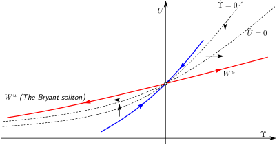
Figure 3. The $(\Upsilon,U)$ phase plane ($n=2$)

Lemma 17.

The Bryant steady soliton is, up to scaling, the unique complete solution of (C.1) satisfying $0<U<1$.

Proof.

It is well known that the Bryant soliton is the unique (up to scaling) complete, rotationally symmetric steady gradient soliton on $\mathbb{R}^{n+1}$, for all $n\geq 2$. The point of the lemma is to exhibit it as a solution of (C.1), i.e. an unstable trajectory of (C.4) emerging from the fixed point $(\Upsilon,U)=(0,1)$.

We write the Bryant soliton $(\mathbb{R}^{n+1},\bar{g},\mathrm{grad}f)$ as it appears in [9, Chapter 1, Section 4], following unpublished work of Robert Bryant. The metric $\bar{g}$ is defined in polar coordinates on $\mathbb{R}^{n+1}\setminus\{0\}\approx(0,\infty)\times\mathcal{S}^{n}$ by

(C.5) $$\bar{g}=ds^{2}+w^{2}(s)\,g_{\mathrm{can}}.$$

The soliton flows along the vector field $\mathrm{grad}f$, where $f$ is the soliton potential function, i.e. the solution of $\mathrm{Rc}(\bar{g})+\bar{\nabla}\bar{\nabla}f=0$. For this to hold, it is necessary and sufficient that $w(s)$ and $f(s)$ satisfy the system

(C.6) $$w_{ss}=w_{s}f_{s}+(n-1)\frac{1-w_{s}^{2}}{w},\qquad f_{ss}=n\frac{w_{ss}}{w}.$$

Because $U>0$ for solutions of interest, we substitute $\sigma=w(s)$ and $U=w_{s}(s)$, thereby transforming (C.3) into (C.5). Then recalling from (C.2) that

$$d\zeta=\,\frac{d\sigma}{\sigma}=\frac{w_{s}}{w}\,ds,$$

one sees that (C.4) becomes

(C.7) $$w_{ss}=w_{s}\frac{\Upsilon}{w}+(n-1)\frac{1-w_{s}^{2}}{w},\qquad\Upsilon_{s}=w_{s}f_{s}+nw_{ss}.$$

The choice $\Upsilon=wf_{s}$ transforms (C.7) into (C.6).

In [9], following Bryant’s work, the Bryant soliton is recovered from a careful analysis of trajectories of the ode system [9, equation (1.48)] corresponding to $x=U$ and $y=nU-\Upsilon$ near the saddle point $(x,y)=(1,n)$ corresponding to $(U,\Upsilon)=(1,0)$. There it is shown that there exists a unique unstable trajectory (corresponding to $U\to 0$ and $\Upsilon\to-\infty$ as $s$ increases) that results in a (non-flat) complete steady gradient soliton. Moreover, this solution is unique up to rescaling. ∎

Let $U:(0,\infty)\to(0,1)$ be a solution of (C.1) which corresponds to the Bryant steady soliton. Every other such solution of (C.1) is given by $U(k\sigma)$ for some $k>0$.

We now note a few simple facts about the behavior of the Bryant steady soliton. Its properties near infinity are well known, but its properties near the origin are not as readily found in the literature.

Lemma 18.

 

1. $U$ is strictly monotone decreasing for all $\sigma>0$.

2. Near $\sigma=0$, $U(\sigma)^{2}$ is a smooth function of $\sigma^{2}$, with the asymptotic expansion

   $$U(\sigma)^{2}=1+b_{2}\sigma^{2}+\frac{n}{n+3}b_{2}^{2}\sigma^{4}+\frac{n(n-1)}{(n+3)(n+5)}b_{2}^{3}\sigma^{6}+\cdots,$$

   where $b_{2}<0$ is arbitrary.

3. Near $\sigma=+\infty$, $U^{2}$ has the asymptotic expansion

   $$U(\sigma)^{2}=c_{2}\sigma^{-2}+\frac{4-n}{n-1}c_{2}^{2}\sigma^{-4}+\frac{(n-4)(n-7)}{(n-1)^{2}}c_{2}^{3}\sigma^{-6}+\cdots,$$

   where $c_{2}>0$ is arbitrary.

Proof.

(1) It is well known (see e.g. [9, Lemma 1.37]) that the sectional curvatures of the Bryant soliton are strictly positive for all $\sigma>0$ and have the same positive limit at the origin. By (A.2), the sectional curvature $K$ of a plane perpendicular to the sphere $\{\sigma\}\times\mathcal{S}^{n}$ and the sectional curvature $L$ of a plane tangent to the sphere $\{\sigma\}\times\mathcal{S}^{n}$ are

$$K=-\frac{UU_{\sigma}}{\sigma}\quad\text{and}\quad L=\frac{1-U^{2}}{\sigma^{2}},$$

respectively. Hence $U^{\prime}(\sigma)<0$ and $U(\sigma)<1$ for all $\sigma>0$.

(2) We showed in Lemma 17 that $U=w^{\prime}$. Because $w$ is an odd function that is smooth at zero [17], $U$ is an even function that is smooth at zero. Thus $U^{2}$ has an asymptotic expansion near $\sigma=0$ of the form

$$U(\sigma)^{2}=1+b_{2}\sigma^{2}+b_{4}\sigma^{4}+b_{6}\sigma^{6}+\cdots.$$

By part (1), we must have $b_{2}<0$. (Arbitrariness of $b_{2}$ corresponds to the invariance of $U$ under the rescaling $\sigma\mapsto k\sigma$.) The remaining coefficients are determined by the equation $\mathcal{F}_{\mathrm{in}}[U^{2}]=0$, which implies that

$$0=\left[2(n+3)b_{4}-2nb_{2}^{2}\right]\sigma^{2}+4\left[(n+5)b_{6}-(n-1)b_{2}b_{4}\right]\sigma^{4}+\cdots.$$

In particular,

$$b_{4}=\frac{n}{n+3}b_{2}^{2}>0\qquad\text{and}\qquad b_{6}=\frac{n-1}{n+5}b_{2}b_{4}<0.$$

The claimed expansion follows.

(3) Let $\xi=\sigma^{-1}$. Then $U$ has an asymptotic expansion near $\xi=0$ of the form

$$U(\sigma)^{2}=c_{0}+c_{2}\xi^{2}+c_{4}\xi^{4}+c_{6}\xi^{6}+\cdots.$$

It is well known (see e.g. [9, Remark 1.36]) that $C^{-1}\sqrt{s}\leq w(s)\leq C\sqrt{s}$ for $s$ bounded away from $0$. This forces $c_{0}=0$. One finds that $\mathcal{F}[U^{2}]=0$ if and only if

$$\xi^{2}U^{2}U_{\xi\xi}^{2}-\frac{1}{2}(\xi U_{\xi}^{2})^{2}-(n-1-3U^{2})\xi U_{\xi}^{2}+2(n-1)(U^{2}-U^{4})=0.$$

This allows $c_{2}>0$ to be arbitrary but forces

$$c_{4}=\frac{4-n}{n-1}c_{2}^{2}\qquad\text{and}\qquad c_{6}=\frac{(n-4)(n-7)}{(n-1)^{2}}c_{2}^{3}.$$

The claimed expansion follows. ∎

In function $\mathfrak{B}$ which we have used extensively in this paper is by definition

(C.8) $$\mathfrak{B}(\sigma)=U(k\sigma)^{2}$$

where $U$ is as above in Lemma 18, and where the constant $k$ is chosen so that

(C.9) $$\mathfrak{B}(\sigma)=\frac{1}{\sigma^{2}}+o(\sigma^{-2}),\qquad(\sigma\to\infty).$$

Lemma 18 implies that such a choice of $k$ exists, and that $\mathfrak{B}$ is thus uniquely defined.

References

- [1] Angenent, Sigurd B.; Knopf, Dan. An example of neck pinching for Ricci flow on . Math. Res. Lett. 11 (2004), no. 4, 493–518.
- [2] Angenent, Sigurd B.; Knopf, Dan. Precise asymptotics of the Ricci flow neckpinch. Comm. Anal. Geom. 15 (2007), no. 4, 773–844.
- [3] Bemelmans, Josef; Min-Oo; Ruh, Ernst A. Smoothing Riemannian metrics. Math. Z. 188 (1984), no. 1, 69–74.
- [4] Bessières, Laurent; Besson, Gerard; Boileau, Michel; Maillot, Sylvain; Porti, Joan. Weak solutions for Ricci flow on compact, irreducible -manifolds. http://www.ihp.jussieu.fr/ceb/Ricci%20T08-2/english_solution.pdf
- [5] Brendle, Simon; Schoen, Richard M. Manifolds with -pinched curvature are space forms. J. Amer. Math. Soc., to appear. (arXiv:0705.0766v3).
- [6] Cao, Huai-Dong; Zhu, Xi-Ping. Hamilton-Perelman’s Proof of the Poincaré Conjecture and the Geometrization Conjecture. arXiv:math/0612069v1. [Authors’ revision of: A complete proof of the Poincaré and geometrization conjectures—application of the Hamilton-Perelman theory of the Ricci flow. Asian J. Math. 10 (2006), no. 2, 165–492.]
- [7] Chen, Xiuxiong; Ding, Weiyue. Ricci flow on surfaces with degenerate initial metrics. J. Partial Differential Equations 20 (2007), no. 3, 193–202.
- [8] Chen, Xiuxiong; Tian, Gang; Zhang, Zhou. On the weak Kähler–Ricci flow. arXiv:0802.0809v1.
- [9] Chow, Bennett; Chu, Sun-Chin; Glickenstein, David; Guenther, Christine; Isenberg, Jim; Ivey, Tom; Knopf, Dan; Lu, Peng; Luo, Feng; Ni, Lei. The Ricci Flow: Techniques and Applications, Part I: Geometric Aspects. Mathematical Surveys and Monographs, Vol. 135. American Mathematical Society, Providence, RI, 2007.
- [10] Chow, Bennett; Chu, Sun-Chin; Glickenstein, David; Guenther, Christine; Isenberg, Jim; Ivey, Tom; Knopf, Dan; Lu, Peng; Luo, Feng; Ni, Lei. The Ricci Flow: Techniques and Applications, Part II: Analtyic Aspects. Mathematical Surveys and Monographs, Vol. 144. American Mathematical Society, Providence, RI, 2008.
- [11] Feldman, Mikhail; Ilmanen, Tom; Knopf, Dan. Rotationally symmetric shrinking and expanding gradient Kähler-Ricci solitons. J. Differential Geom. 65 (2003), no. 2, 169–209.
- [12] Gu, Hui-Ling; Zhu, Xi-Ping. The Existence of Type II Singularities for the Ricci Flow on . Comm. Anal. Geom. 16 (2008), no. 3, 467–494.
- [13] Hamilton, Richard S. The formation of singularities in the Ricci flow. Surveys in differential geometry, Vol. II (Cambridge, MA, 1993), 7–136, Internat. Press, Cambridge, MA, 1995.
- [14] Hamilton, Richard S. A compactness property for solutions of the Ricci flow. Amer. J. Math. 117 (1995), no. 3, 545–572.
- [15] Hamilton, Richard S. Four-manifolds with positive isotropic curvature. Comm. Anal. Geom. 5 (1997), no. 1, 1–92.
- [16] Huisken, Gerhard; Sinestrari, Carlo. Mean curvature flow with surgeries of two–convex hypersurfaces. Invent. Math. 175 (2009), no. 1, 137-221.
- [17] Ivey, Thomas. On solitons for the Ricci Flow. Ph.D. dissertation, Duke University, 1992.
- [18] Kleiner, Bruce; Lott, John. Notes on Perelman’s papers. arXiv:math/0605667.
- [19] Koch, Herbert; Lamm, Tobias. Geometric flows with rough initial data. arXiv:0902.1488v1.
- [20] Ladyženskaja, O.A.; Solonnikov, V.A.; Uralćeva, N. N. Linear and quasilinear equations of parabolic type. (Russian) Translated from the Russian by S. Smith. Translations of Mathematical Monographs, Vol. 23 American Mathematical Society, Providence, R.I. 1967.
- [21] Morgan, John; Tian, Gang. Ricci flow and the Poincaré conjecture. Clay Mathematics Monographs, 3. American Mathematical Society, Providence, RI; Clay Mathematics Institute, Cambridge, MA, 2007.
- [22] Perelman, Grisha. The entropy formula for the Ricci flow and its geometric applications. arXiv:math.DG/0211159.
- [23] Perelman, Grisha. Ricci flow with surgery on three-manifolds. arXiv:math.DG/0303109.
- [24] Perelman, Grisha. Finite extinction time for the solutions to the Ricci flow on certain three-manifolds.
- [25] Schnürer, Oliver C.; Schulze, Felix; Simon, Miles. Stability of Euclidean space under Ricci flow. arXiv:0706.0421.
- [26] Simon, Miles. A class of Riemannian manifolds that pinch when evolved by Ricci flow. Manuscripta Math. 101 (2000), no. 1, 89–114.
- [27] Simon, Miles. Deformation of Riemannian metrics in the direction of their Ricci curvature. Comm. Anal. Geom. 10 (2002), no. 5, 1033–1074.
- [28] Simon, Miles. Ricci flow of almost non-negatively curved three manifolds. arXiv:math/0612095.
- [29] Shi, Wan-Xiong. Deforming the metric on complete Riemannian manifolds. J. Differential Geom. 30 (1989), no. 1, 223–301.
- [30] Tao, Terence. Perelman’s proof of the Poincaré conjecture: a nonlinear PDE perspective. arXiv:math/0610903.
- [31] Topping, Peter. Ricci flow compactness via pseudolocality, and flows with incomplete initial metrics. J. Eur. Math. Soc. (JEMS), to appear. 555http://www.warwick.ac.uk/~maseq/topping_rfse_20071122.pdf