Primitive turbulence: kinetics, Prandtl’s
mixing length, and von Kármán’s constant

Abstract

The paper presents a theory of shear-generated turbulence at asymptotically high Reynolds numbers. It is based on an ensemble of dipole vortex tubes taken as quasi-particles and realized in form of rings, hairpins or filament couples of potentially finite length. In a not necesserily planar cross sectional area through a vortex tangle, taken locally orthogonal through each individual tube, the dipoles are moving with the classical dipole velocity $u=r\cdot\omega$. The vortex radius $r$ is directly related with Prandtl’s classical mixing length. The quasi-particles perform dipol chaos which reminds of molecular chaos in real gases. Collisions between quasi-particles lead either to particle annihilation (turbulent dissipation) or to particle scattering (turbulent diffusion). These ideas suffice to develop a closed theory of shear-generated turbulence without empirical parameters, with analogies to birth and death processes of macromolecules. It coincides almost perfectly with the well-known $K$-$\Omega$ turbulence closure applied in many branches of science and technology. In the case of free homogeneous decay the TKE is shown to follow $t^{-1}$. For an adiabatic condition at a solid wall the theory predicts a logarithmic mean-flow boundary layer with von Kármán’s constant as $(2\,\pi)^{-1/2}\approx 0.399$.

“Everything should be made as simple as possible, but not simpler.”

– Albert Einstein

Keywords: Turbulence, vortex dipoles, vortex gas, dipol chaos, quasi-particles, von Kármán’s constant, law of the wall

Baumert Primitive turbulence H. Z. Baumert, IAMARIS, Bei den Mühren 69A, D-20457 Hamburg, Germany (baumert@iamaris.de)

1 Introduction

"The diversity of problems in turbulence should not obscure the fact that the heart of the subject belongs to physics." (Falkowski and Sreenivasan 2006). Most classical turbulence theories and models rest more or less on the Fridman-Keller (1924) series expansion of the Navier-Stokes equation, the first element of which is the Reynolds (1895) equation. Higher elements are the subject of turbulence closure models (e.g. Wilcox 2006). This approach attracted many researchers, but could not solve most elementary problems of turbulence. On the contrary, it led to more and more ‘universal’ higher-order equations. Although also the writer of this article made his first steps towards turbulence along this path, he became more and more sceptic that it is the right one to proceed. Therefore, with the exception of the mean-flow kinetic energy balance, the following text does not take much advantage from the Fridman-Keller expansion.

Below a new path is testet. It is mathematiclly simple, and for some readers even primitive so that the writer felt obliged to announce this already in the headline. Nevertheless, a primitive model sometimes highlights aspects which are overseen in more elaborate theories (Lorenz 1960).

The following development explores physical analogies between turbulence taken as an ensemble of vortex-dipol tubes and real gases of semi-stable macromolecules. The underlaying non-linear statistical theory of macromolecular gas kinetics is not repeated here and can be found, for example, in textbooks on synergetics (Haken 1978) .

While in ideal gases molecules are point masses with zero cross section and infinite free path, in real gases the cross sections are finite so that molecule-molecule collisions limit the free path. A collision of two molecules (higher-order collisions are neglected here for simplicity) can have one out of two possible results:

• The molecules are spatially scattered, which corresponds to molecular diffusion and mixing.

• The molecules vanish due to their semi-stability, which corresponds to particle annihilation or concentration decay.

The turbulent analogues of the above two processes are (i) turbulent diffusion and (ii) annihilation of vortices or dissipation of turbulent kinetic energy. The particle dynamics (molecules, vortices) can be described by the following equation, which is a special case of the Oregonator (a certain class of diffusion-reaction systems, see e.g. Ch. 9 in Haken, 1978):

$$\frac{\partial n}{\partial t} = \frac{\partial}{\partial\vec{x}}\left(\nu\,\frac{\partial n}{\partial\vec{x}}\right)-\beta\,n^{2}\,.$$ (1)

Here $n$ is the particles’ volume density, $\nu$ is the diffusivity, and $\beta$ is a constant.

Equation (1) describes the joint effect of two irreversible processes: particle diffusion through ${\partial}/{\partial\vec{x}}\left(\nu\,{\partial n}/{\partial\vec{x}}\right)$, and irreversible decay through $-\beta\,n^{2}$. It forms an initial-value problem for $n=n(\vec{x},t)$. The final state is $n(\vec{x},\infty)=0$. Finite molecule numbers can only be kept when new particles are continuously added to the volume under study.

The following theory uses discrete vortex dipoles instead of the a.m. semi-stable macromolecules. They are quasi-particles, i.e. locally excited states of an otherwise homogeneous fluid like phonons in solid-state physics. At very high Reynolds number $Re$ we expect that the fluid contains asymptotically many vortices and exhibits universal behavior in the sense of the Kolmogorov (1941) scaling laws.

2 Vortices

The classical closed vortex line (e.g. the closed centerline of an idealized smoke ring) represents an exact weak solution of the Euler equation, has infinitely thin diameter, infinitely high angular velocity, but finite circulation, $c=\pi\,r^{2}\,\omega<\infty$, where $r$ and $\omega$ are effective radius and vorticity. The fluid outside the vortex line is inviscid and irrotational. The classical vortex is an abstract frictionless object.

The Batchelor couple (Lesieur 1997) is a vortex dipol, consisting of two anti-parallel vortex lines. It is also an idealized frictionless object. When isolated and far from boundaries, in 3D the trajectory of a Batchelor couple is a straight line. The flow field of one vortex moves the other vortex and vice versa. In practice such couples are stable over short to moderate propagation times. They conserve their kinetic energy, circulation (which is zero for this couple by definition), their vortex radii and vorticities (which carry opposite signs). The Batchelor couple propagates into the same direction as the fluid moves between the two vortices forming the couple. In a sufficiently dense ensemble of Batchelor couples their trajectories are no longer straight lines due to mutual interactions.

The counterpart of the Batchelor couple will be called below a von-Kármán couple. It is a pair of parallel vortex lines of non-zero total circulation. In an initial phase of their evolution they rotate around their common center of gravity, which remains in rest. Such a couple is known since long to be fundamentally unstable. Its kinetic energy is dissipated into heat (e.g. Lamb 1932) .

2.1 Vortex dipoles $vs.$ vorticons

A vorticon is a narrow relative of the Batchelor couple, with the following differences: the effective radius $r$ and its kinetic energy $u^{2}/2=r^{2}\omega^{2}/2$ are finite. These conditions are well realized in practice, at best in quantum turbulence (cf. Vinen and Donelly 2007) .

Vorticon generation = turbulence production: Due to the conservation principle for circulation in ideal fluids (Helmholtz 1858), in a circulation-free volume vortices can be generated (and annihilated) only in form of anti-parallel vortex pairs with vanishing circulation. I.e. turbulence kinetic energy (TKE) generation by shear is generation of quasi-particles in the above sense.

Vorticon annihilation = TKE dissipation: Vorticons can be annihilated in collisions if the two collision partners are reorganized into von-Kármán couples. Consider two initial vorticons, $(+\Uparrow-)^{1}$ and $(-\Downarrow+)^{2}$, which reorganize during collision into the following von-Kármán couples: ($+^{1}\;\|\;+^{2}$) and ($-^{1}\;\|\;-^{2}$), where the numbers ¹ and ² refer to the numbered particles. In both new ‘particles’ the non-zero molecular viscosity of a real fluid leads to kinetic energy dissipation and finally to a merger of the like-signed vortices on a lower energy level (see also Klein & Majda 1993). This ‘inelastic’ collision happens when the angle $\varphi$ between the propagation directions of the two colliding vorticons belongs to the interval $\frac{1}{2}\,\pi\leq\varphi<\frac{3}{2}\,\pi$ (forward facing half sphere).

In the initial definition of our quasi-particles we have neglected viscosity. We re-introduce this important property by assuming that von-Kármán couples are absolutely instable and instantaneously converted into heat.

Vorticon scattering = turbulent diffusion: Vorticons are scattered in collisions between two vorticons if the two are reorganized into two new Batchelor couples with new propagation angles. Consider again two initial vorticons, $(+\Uparrow-)^{1}$ and $(-\Downarrow+)^{2}$. After a collision they may form a new quasi-particle with a new propagation velocity vector: ($+^{1}\;\|\;-^{2}$) and ($-^{1}\;\|\;+^{2}$). This ‘elastic’ collistion happens when the angle $\varphi$ between the propagation directions of the two colliding vorticons belongs to the backward facing half sphere.

2.2 Vorticon tangle

At high $Re$ vorticons are assumed to form a dense three-dimensional tangle. As already found for 2D trajectories (Aref 1983, Eckhardt and Aref 1988) , in 3D vorticons as elements of a tangle propagate along complex non-linear trajectories until collision with other vorticons. But we expect that the tangle is so dense that the effective trajectories are short and can be treated as straight lines. Frisch (1995) suggested that “The idea of conservative dynamics punctuated by dissipative events could be directly relevant in three dimensions.” This is exactly what is elaborated here. Our form of ‘conservative dynamics’ is chaotic dipol motion which conserves energy until particle annihilation. The trajectories are ‘punctuated’ by dissipative collisions which lead to vorticon conversion into heat.

Figure 1 exhibits a cross section through vorticons. The arrows denote the propagation direction. A plus sign indicates rotation against the clock.

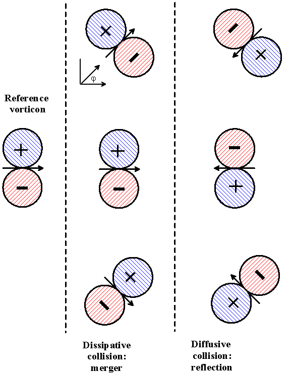
Figure 1: Two elementary vorticon-vorticon interactions. On the very left the reference vorticon is shown which is assumed to move to the right. The middle column shows different orientations of the target vorticon which all lead to a dissipative (inelastic) collision, i.e. to annihilation of a quasi-prarticle. The right column shows potential target vorticons in elastic scatter position corresponding to turbulent diffusion. A collision with these targets conserves energy.

2.3 Historical notes

Whereas the present approach to turbulence is based on ensembles of $discrete$ quasi-particles, most turbulence closures of the past take the fluid as a $continuum$. Both concepts are old. James Clerk Maxwell (1867) gave a detailed discussion of this dichotomy in connection with his kinetic theory of gases and traced it back to Democrit and Lucretius. René Descartes (1596 – 1650) spoke about ‘tourbillons’ forming the universe; based on the results of Herrmann von Helmholtz (1858) Lord Kelvin (1867a, b) coined the notion ‘vortex atoms’; for a comprehensive overview see (Saffman 1992) .

Most of later analytic efforts towards a kinetic theory of vortices were restricted to spatially two-dimensional cases wherein the Hamilton formalism is applicable (Onsager 1949) . Exceptions are vortex-based numerical simulation receipes and rules.

Marmanis (1998) was the first who proposed the vortex dipole as $the$ fundamental quasi-particle of turbulence. He wrote: "The introduction of the vortex dipole chaos assumption permits one to derive a kinetic equation for a ‘gas’ of vortex dipoles." He presented a methodical mixture of Onsager’s theory with Bogoljubov’s perturbation-kinetic approach with application to 2D inviscid turbulence. Dissipative 3D turbulence has not been treated by this author.

Lions and Majda (2000) tried to develop a kinetic theory of 3D turbulence at high $Re$. They used systematic asymptotic expansions of the Navier-Stokes equation in the Fridman-Keller sense. On the one hand they tried to overcome limitations of the Klein-Majda theory (Klein and Majda 1993) , on the other hand they limited themselves to the quasi-parallel case where the Klein-Majda theory is constructively applicable through a rigorous equilibrium statistical formalism.

Chen et al. 2004 also aimed at the development of a physico-kinetic turbulence theory. They explicitely envisaged Boltzmann’s approach and developed a complex formalism, but still without practically applicable predictions.

Despite high efforts, these works did not yet lead to unique and constructive rules for the practical computation of the eddy viscosity from mean flow data. Unfortunately, with a few exceptions eddy viscosity is the most important turbulence parameter in computational aero-, hydro- and thermo-dynamics.

Below turbulence balance equations are derived which describe the local-average dynamics of turbulence kinetic energy, $K$, mean vorticity, $\omega$, and eventually eddy viscosity, $\nu$. These equations are only a specific format or a specific implementation of the primitive theory. In special cases they can be solved analytically.

In more general cases one would try to solve them using finite-difference or finite-volume etc. methods. If the solution shall be approximated by the Monte-Carlo method then the writer recommends to start not from the continuum equations derived below, but better directly from the mechanical picture of the vorticon ensemble, preferably using the already existing eddy-collision methods where various vortex-filament primitives are already avaialable (Cottet and Koumoutsakos 2000, Andeme 2008).

3 Primary variables in primitive turbulence

3.1 TKE and vorticity

For the construction of the eddy viscosity, which is proportional to TKE $times$ unit time, and of the TKE dissipation rate, which is TKE $per$ unit time, two constituing variables are necessary: TKE and a measure of time. Here the below-defined quantities $K$ and $\omega$ are chosen. They are introduced now.

Consider a small volume element $\delta V$ populated by an ensemble of $j=1\dots n$ dipoles with individual effective vortex radii $r_{j}$ and vorticities $\omega_{j}$. During the free flight time $\tau_{j}$ the properties of the quasi-particle $j$ are conserved. The particle’s volume density is $n/\delta\cal V$. The total TKE within $\delta\cal V$ is the sum of the kinetic energies of the individual vorticons:

$$K_{\delta\cal V} = \frac{1}{\delta\cal V}\sum_{j\epsilon\delta\cal V}\frac{1}{2}\,r_{j}^{2}\,\omega_{j}^{2}\;=\;\frac{n}{\delta\cal V}\;\bar{k}\;,$$ (2)

$$\omega_{\delta\cal V} = \frac{1}{\delta\cal V}\sum_{j\epsilon\delta\cal V}|\omega_{j}|\;=\;\frac{n}{\delta\cal V}\;\bar{\omega}\,.$$ (3)

Multiplication of (2, 3) with $\delta\cal V$ gives

$$K\;=\;\delta\cal V\cdot K_{\delta\cal V} = \sum_{j\epsilon\delta\cal V}\frac{1}{2}\,r_{j}^{2}\,\omega_{j}^{2}\;=\;n\;\bar{k}\;,$$ (4)

$$\omega\;=\;\delta\cal V\cdot\omega_{\delta\cal V} = \sum_{j\epsilon\delta\cal V}|\omega_{j}|\;=\;{n}\;\bar{\omega}\,.$$ (5)

$K_{\delta\cal V}$, $\omega_{\delta\cal V}$ are local volume densities of TKE and vorticity magnitude, respectively. They and $K,$ $\omega$ are extensive variables by definition, i.e. they change when new particles with average properties $\bar{k}$, $\bar{\omega}$ are added to $\delta\cal V$, as then $K\rightarrow(n+1)\,\bar{k}$ and $\omega\rightarrow(n+1)\,\bar{\omega}$.

$\bar{k}$ and $\bar{\omega}$ are ensemble averages and as such intensive variables which do not change when new particles with average properties are added to the ensemble in $\delta\cal V$:

$$\bar{k} = \frac{1}{n}\sum_{j\epsilon\delta\cal V}\frac{1}{2}\,r_{j}^{2}\,\omega_{j}^{2}\,,$$ (6)

$$\bar{\omega} = \frac{1}{n}\sum_{j\epsilon\delta\cal V}|\omega_{j}|\,.$$ (7)

3.2 Auxiliary quantities

We introduce useful auxiliary quantities: the ordinary vorticity frequency, $\Omega=1/T$ and the often used constant $\kappa$:

$$\omega = 2\,\pi\,\Omega\;=\;\Omega/\kappa^{2}\,,$$ (8)

$$\kappa = (2\,\pi)^{-1/2}\approx\,0.399\,\,.$$ (9)

Further below, $\kappa$ appears to be von Kármán’s constant. While $|\omega_{j}|=2\pi/T_{j}$ is an angular frequency, $\Omega$ is an ordinary frequency.

3.3 Derived variables

Effective radius $R$. $R^{2}$ is defined here as the weighted ensemble mean:

$$R^{2} = \frac{\sum_{j\epsilon\delta\cal V}\;r_{j}^{2}\,\omega_{j}^{2}}{(\sum_{j\epsilon\delta\cal V}\;|\omega_{j}|)^{2}}\;=\;\frac{2\,K}{\omega^{2}}\;=\;\frac{2\,\bar{k}}{\bar{\omega}^{2}}\;n^{-1}\,.$$ (10)

It depends (inversely) on $n$ and is thus an extensive variable. In freely decaying homogeneous turbulence (Section 4) only the particle number decreases while the ensemble mean properties $\bar{k}$ and $\bar{\omega}$ remain constant in time such that

$$n\,\pi\,R^{2} =$$ const. (11)

This reminds of a 2D version of the equation of state of a real gas telling us that the (planarized) locally orthogonal cross sectional area through a dense vorticon tangle is compactly filled with dipoles.

Dissipation rate. The rate of TKE dissipation, $\varepsilon$, has the units of TKE per time [m² s^-3]. Up to a factor $\zeta$ it is governed by the product $K\cdot\Omega$, :

$$\varepsilon = \zeta\,\frac{K\,\Omega}{\pi}\;=\;\zeta\,\frac{\bar{k}\,\bar{\omega}}{\pi}\,n^{2}\,.$$ (12)

$\varepsilon$ is an extensive variable. Below we show that $\zeta\equiv 1$. In freely decaying homogeneous turbulence (12) is identical with the quadratic term in (1) such that in this case

$$\beta=\zeta\,\bar{k}\,\bar{\omega}/\pi\;=\;\mbox{const.}$$ (13)

Eddy viscosity. Ludwig Prandtl (1925) noticed two simultaneous properties of his mixing length, namely that it (a) “…may be considered as the diameter of the masses of fluid moving as a whole in each individual case; or again, as the distance traversed by a mass of this type before it becomes blended in with neighboring masses …”; and also that it is (b) “…somewhat similar, as regards effect, to the mean free path in the kinetic theory of gases …” (Bradshaw 1974).

We interpret Prandtl’s mxing length in terms of ‘our’ $R$ in (10) because it is proportional to (a) the local mean radius of vorticons and, simultaneously, (b) to the free path.

To explore this idea further we follow Albert Einstein’s (1905) theory of molecular diffusion in fluids and use his expression for the coefficient of diffusion now for our coefficient of turbulent diffusion, or eddy viscosity $\nu$, in terms of a mean free path, $\lambda$, and a mean free flight time, $\tau$:

$$\nu = {\lambda^{2}}/{2\,\tau}\,\,.$$ (14)

For a vortex dipole these parameters can directly be given as follows wherein $u$ is the mean (linear) advection velocity of a vortex dipole:

$$\tau = {\lambda}/{u}\,,$$ (15)

$$u = \sqrt{2\,K}\,.$$ (16)

For a quasi-steady turbulent vorticon tangle at $Re=\infty$ and far from solid boundaries the mean free path will clearly be very limited but it cannot vanish. The packing density should be dense but small enough that during a flight a particle can be replaced by a newly generated. This implies that (Baumert 2005b)

$$\lambda = 2\,R\,.$$ (17)

The free area of a free vorticon far from boundaries is (Fig. 2)

$${\cal A}_{free} = (4\,R)^{2}\,.$$ (18)

We finally get the eddy viscosity as an intensive variable as follows:

$$\nu = K/\pi\,\Omega\;=\;2\,K/\omega\;=\;\omega\;R^{2}\,,$$ (19)

This equation is called the Prandtl-Kolmogorov relation.

4 Free homogeneous decay of turbulence

For constant properties $\bar{k}$, $\bar{\omega}$ of our quasi-particles, following (6, 7) the variables $K$ and $\Omega$ are proportional to the vorticon density $n$ and have therefore to satisfy the same diffusion-reaction equation (1) like $n$, because these properties are ‘solidly mounted’ at the dipoles. In the case of decay we have thus the following:

$$n\;=\;\frac{K}{\bar{k}}\;=\;\frac{\omega}{\bar{\omega}}\,.$$ (20)

In analogy to (1) it holds that

$$\frac{dK}{dt}+\beta_{K}\,K^{2} = 0\;,$$ (21)

$$\frac{d\Omega}{dt}+\beta_{\Omega}\,\Omega^{2} = 0\;.$$ (22)

The reader easily sees that at large $t$

$$K(t) = (\beta_{K}\,t)^{-1}\;,$$ (23)

$$\Omega(t) = (\beta_{\Omega}\,t)^{-1}\;,$$ (24)

and

$$\nu(t) = \frac{K(t)}{\pi\,\Omega(t)}\;=\;\frac{\beta_{\Omega}}{\pi\,\beta_{K}}\;=\;\mbox{const.}$$ (25)

Equation (23) coincides with the results of a fairly general similarity analyses of the Navier-Stokes equations by Oberlack (2002) and with the experimental results of Dickey and Mellor (1980).

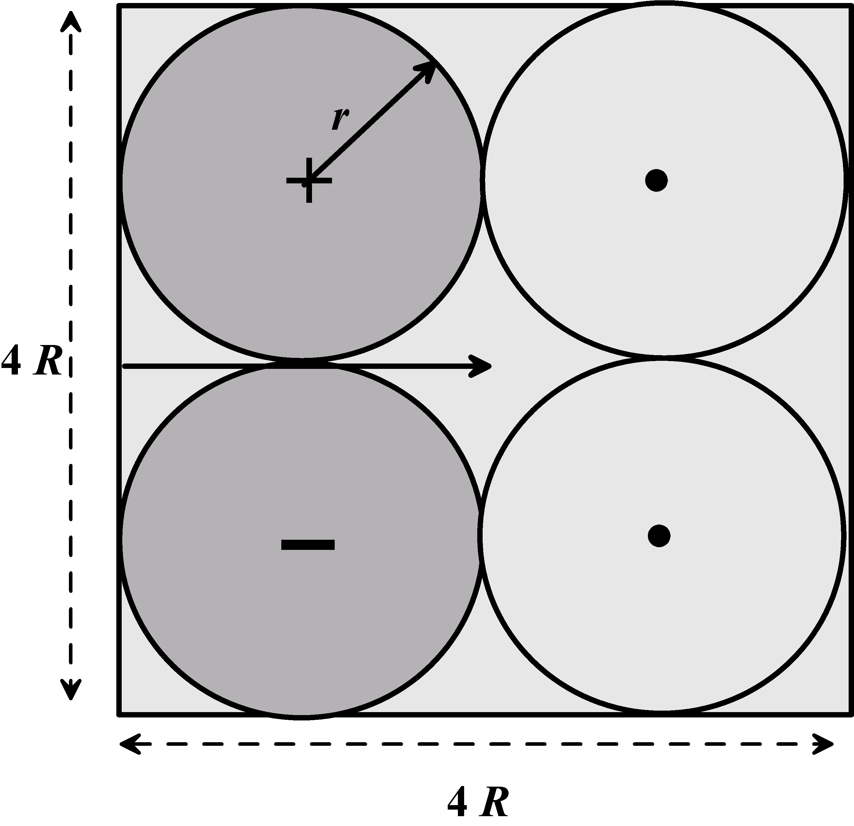
Figure 2: Local cross section through a dipol tangle far from boundaries with maximum possible density at $Re\rightarrow\infty$. The dark grey vorticon in the left half square labelles the instantaneous situation, the ‘empty vorticon’ in the right half square indicates the vorticon after its free flight from the left to the right into its collision position, where it is either annihilated or scattered. Far from boundaries a vorticon obviously ‘needs’ a cross sectional area of ${\cal A}_{free}=(4\,R)^{2}$).

5 Forced inhomogeneous turbulence

In contrast to Section 4 now the assumptions of free decay and spatial homogeneity are given up. This implies that we need to add source ($F_{K}$ and $F_{\Omega}$) and diffusion terms to the right-hand sides of equations (21, 22):

$$\frac{\partial K}{\partial t}+\beta_{K}\,K^{2} = F_{K}+\frac{\partial}{\partial\vec{x}}\left(\nu\,\frac{\partial K}{\partial\vec{x}}\right),$$ (26)

$$\frac{\partial\Omega}{\partial t}+\;\beta_{\Omega}\,\Omega^{2} = F_{\Omega}+\frac{\partial}{\partial\vec{x}}\left(\nu\,\frac{\partial\Omega}{\partial\vec{x}}\right)\,.$$ (27)

The factors $\beta_{K}$ and $\beta_{\Omega}$ are not longer expected to be constants.

5.1 TKE production by mean-flow shear: $F_{K}$

The specification of the TKE production term $F_{K}$ for a shear flow can be obtained from textbooks (Wilcox 2006, Schlichting and Gersten 2000),

$$F_{K}\;=\;\nu\,S^{2}\;=\;\frac{K}{\pi\,\Omega}\,S^{2}\,,$$ (28)

where $S^{2}$ is the total instantaneous shear, squared,

$$S^{2}\;=\;\sum_{i,j=1}^{3}\left(\frac{\partial U_{j}}{\partial x_{i}}+\frac{\partial U_{i}}{\partial x_{j}}\right)\;\frac{\partial U_{i}}{\partial x_{j}}\,,$$ (29)

and $U_{i}$ is the $i^{th}$ component of the mean flow velocity vector $(U_{1},U_{2},U_{3})^{T}$.

5.2 Vorticity generation by mean-flow shear: $F_{\Omega}$

The above formula (28) for $dK/dt=F_{K}$ is classical hydrodynamic knowledge. However, the specification of the vorticity generation term $F_{\Omega}$ is less trivial. Here one has to consider a fundamental argument of Henry Tennekes. It has been carefully discussed in the past, see Tennekes 1989; Baumert and Peters 2000, 2004; Kantha 2004, 2005; Kantha et al. 2005; Kantha and Clayson 2007. We cast Tennekes’ argument into mathematical form. He hypothesized that, on dimensional grounds, the length scale (here: $L$ or $R$) cannot depend on the ambient shear for a neutrally stratified homogeneous shear flow. Since shear production $F_{K}$ involves shear, $F_{\Omega}$ needs to be constructed such that the role of shear vanishes in the evolution equation for the length scale. The latter is generally derived from equation (10) as

$$\frac{1}{R^{2}}\,\frac{dR^{2}}{dt}\;=\;\frac{1}{K}\,\frac{dK}{dt}-2\,\frac{1}{\omega}\,\frac{d\omega}{dt}\,.$$ (30)

We insert $dK/dt$ from (28) in (30) and find

$$\frac{1}{R^{2}}\,\frac{dR^{2}}{dt}\;=\;\frac{S^{2}}{\pi\,\Omega}-2\,\frac{1}{\omega}\,\frac{d\omega}{dt}\,.$$ (31)

In terms of the present theory, Tennekes’ hypothesis means $dR^{2}/dt=0$, which implies that

$$\frac{S^{2}}{\pi\,\Omega}\;=\;2\,\frac{1}{\omega}\,\frac{d\omega}{dt}\,.$$ (32)

It is left to the reader to see that (32) gives

$$\frac{d\Omega}{dt} = \frac{S^{2}}{2\,\pi}\,.$$ (33)

As far as (10) is a pure ensemble-mean definition which considers neither diffusion nor annihilation of particles, the time derivative in (33) needs to be understood as the pure generation term in (27), $F_{\Omega}$:

$$F_{\Omega} = \frac{S^{2}}{2\,\pi}\,.$$ (34)

5.3 The multipliers $\beta_{K}$ and $\beta_{\Omega}$

Let us summarize (26, 27) and (28, 34) as follows,

$$\frac{\partial K}{\partial t}-\frac{\partial}{\partial\vec{x}}\left(\nu\,\frac{\partial K}{\partial\vec{x}}\right) = \frac{K}{\pi\,\Omega}\,S^{2}-\beta_{K}\,K^{2}\,,$$ (35)

$$\frac{\partial\Omega}{\partial t}-\frac{\partial}{\partial\vec{x}}\left(\nu\,\frac{\partial\Omega}{\partial\vec{x}}\right) = \frac{S^{2}}{2\pi}-\beta_{\Omega}\,\Omega^{2}\,.$$ (36)

where $\nu$ is known as function of $K$ and $\Omega$ through (19). It remains to determine the still unknown multipliers $\beta_{K}$ and $\beta_{\Omega}$. This can be accomplished as follows.

We note that the term $\beta_{K}\,K^{2}$ in (35) is identical with the dissipation rate (12) of TKE:

$$\varepsilon = \zeta\,\frac{K\,\Omega}{\pi}\;=\;\beta_{K}\,K^{2}\,.$$ (37)

From the second equation in (37) we conclude with (19) that

$$\beta_{K}\;=\;\frac{\zeta}{\nu\,\pi^{2}}\,,$$ (38)

while from (25) it follows that

$$\beta_{\Omega}\;=\;\nu\,\pi\,\beta_{K}\,.$$ (39)

We insert (38) into (39) and see that

$$\beta_{\Omega}\;=\;\frac{\zeta}{\pi}\,.$$ (40)

Inserting (38, 40) in (35, 36) we get, after some algebra using (19), an almost complete system wherein only $\zeta$ is still to be specified:

$$\frac{\partial K}{\partial t}-\frac{\partial}{\partial\vec{x}}\left(\nu\,\frac{\partial K}{\partial\vec{x}}\right) = \nu\left(S^{2}-\zeta\,\Omega^{2}\right),$$ (41)

$$\frac{\partial\Omega}{\partial t}\;-\frac{\partial}{\partial\vec{x}}\left(\nu\,\frac{\partial\Omega}{\partial\vec{x}}\right) = \frac{1}{\pi}\left(\frac{1}{2}\,S^{2}-\zeta\,\Omega^{2}\right).$$ (42)

6 Turbulent boundary layer

Consider a stationary boundary layer close to a plane solid wall at $z=0$ where $z$ is the only coordinate of interest here. It points orthogonal from the wall into the fluid. The mean flow is parallel to the wall, i.e. $U_{1}=U>0$ and $U_{2}=U_{3}=0$. Consequently with (29) we have to write

$$S\;=\;\left|dU/dz\right|.$$ (43)

The diffusive TKE flux into the viscous sublayer at $z=z_{0}\rightarrow 0$ has to vanish,

$$\left(\nu\,dK/dz\right)_{z=z_{0}}\;=\;0\,,$$ (44)

or

$$K(z)\;=\;K_{0}\;=\;\mbox{const.}$$ (45)

such that in the stationary case (41) gives

$$\Omega\;=\;S/\sqrt{\zeta}\,.$$ (46)

6.1 Logarithmic law of the wall

We insert (46) into the stationary form of (42) so that we have to solve the following equation for $S=S(z)$:

$$\frac{2\,K_{0}}{2\,\zeta-1}\,\frac{d}{dz}\left(\frac{1}{S}\,\frac{dS}{dz}\right)\;=\;S^{2}\,.$$ (47)

The solution is

$$S(z)\;=\;\frac{dU}{dz}\;=\;\frac{\sqrt{2\,K_{0}/(2\,\zeta-1)}}{z}\,.$$ (48)

Integration of (48) gives the logarithmic law of the wall. In boundary layer theory the bottom shear stress is mostly defined in terms of the squared friction velocity, $u_{f}^{2}$,

$$u_{f}^{2}\;=\;\nu\,\frac{dU}{dz}\;=\;\frac{K_{0}}{\pi\,\Omega}\,S\,,$$ (49)

and with (46) it follows that

$$K_{0}\;=\;\pi\,u_{f}^{2}/\sqrt{\zeta}\,.$$ (50)

This allows to rewrite (48) as follows,

$$S(z)\;=\;\frac{dU}{dz}\;=\;\frac{u_{f}}{\tilde{\kappa}\,z}\,,$$ (51)

with $\tilde{\kappa}$ defined through

$$\tilde{\kappa}\;=\;\kappa\,\sqrt{(2\zeta-1)\sqrt{\zeta}}\,.$$ (52)

Integration of (51) provides us with

$$U(z)\;=\;\frac{u_{f}}{\tilde{\kappa}}\,\ln\left(\frac{z}{z_{0}}\right).$$ (53)

6.2 Mixing length $L$

Consider the definition of the effective vorticon radius through (10). We solve this equation for $K$ and express the TKE in terms of $R$ and $\Omega$ as follows:

$$K\;=\;2\,\pi^{2}\,R^{2}\,\Omega^{2}\,.$$ (54)

In practical analyses of boundary layer turbulence, Prandtl’s (1925) concept of mixing length is still often applied. It relates the eddy viscosity to the shear. Following Hinze (1959, p. 279, eq. 5-2) in present notation, Prandtl defined his mixing length $L$ as follows:

$$\nu\;=\;L^{2}\,\left|\frac{dU}{dz}\right|\;=\;L^{2}\,S\,.$$ (55)

Due to our eddy viscosity formula (19) relation (55) gives

$$L^{2}\;=\;\frac{K}{\pi\,\Omega\,S}\,,$$ (56)

so that in the neighborhood of a solid wall we get with (46) the following result:

$$K\;=\;\pi\,L^{2}\,\Omega^{2}\,\sqrt{\zeta}\,.$$ (57)

Equating (54) with (57) gives

$$L\;=\;\frac{R}{\kappa}\,\zeta^{\,-1/4}\,.$$ (58)

The physical meaning of $L$ is easily understood by a glance at Fig. 3. If we may set $\zeta=1$ then (58) gives together with the definition of $\kappa$ in (9) the following,

$$L^{2}=2\,(\pi\,R^{2})\,,$$ (59)

which is the area of a vorticon, fully compressed into the form of a square of side length $L$. This is the asymptotically maximum deformation which justifies to set $\zeta\equiv 1$.

While Prandtl’s mixing-length concept was applicable only in the vicinity of solid boundaries so that it attracted respectful criticism (e.g. Kundu 1990, p. 457; Wilcox 2006), our concept is a generalization of Prandtl’s concept and works also far from boundaries, even in the free stream of stratified fluids where $L$ may approach the Thorpe scale and/or the Ozmidov scale, depending on the conditions (Baumert and Peters 2004).

This section shall be closed with a summary of formulae relevant at solid boundaries, where $z$ the distance from the wall:

$$\nu = u_{f}\,L\,,$$ (60)

$$L = \kappa\,z\,,$$ (61)

$$z = L/\kappa\;=\;R/\kappa^{2}\,.$$ (62)

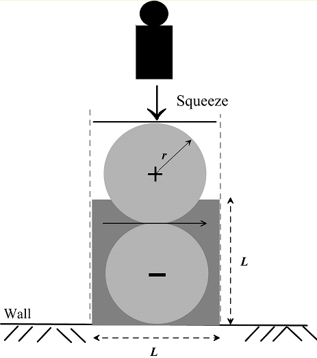
Figure 3: Cross section through a vorticon sheet at a solid boundary. In this Figure we have $r=R$, i.e. the sketched quasi-particle is to be understood as an ensemble average.

6.3 Boundary compression

Far from boundaries the dipole chaos is isotropic and a vorticon’s cross section exhibits circles (Fig. 1). Closer to a solid wall symmetry is increasingly broken and we see ellipses instead. Right at the boundary the ellipses are even deformed to an equivalent square (the asymptotic case) with side length $L=(2\,\pi\,R^{2})^{1/2}$, Fig. 3. This is the minimum area a vorticon can asymptotically attain:

$${\cal A}_{bound}=L^{2}=2\,\pi\,R^{2}\,.$$ (63)

Notice that the fluid within the vorticon is free of friction so that circle, ellipse and square are energetically identical.

To estimate the degree of boundary compression of vorticons quantitatively we compare area (18) ‘occupied’ by a free vorticon far from boundaries with the corresponding area (63) for a compressed vorticon at the very boundary:

$$\frac{{\cal A}_{free}}{{\cal A}_{bound}}\;=\;\frac{(4\,R)^{2}}{2\,L^{2}}\;=\;\frac{16\,R^{2}}{4\,\pi\,R^{2}}\;=\;\frac{4}{\pi}\,\approx 1.27\,.$$ (64)

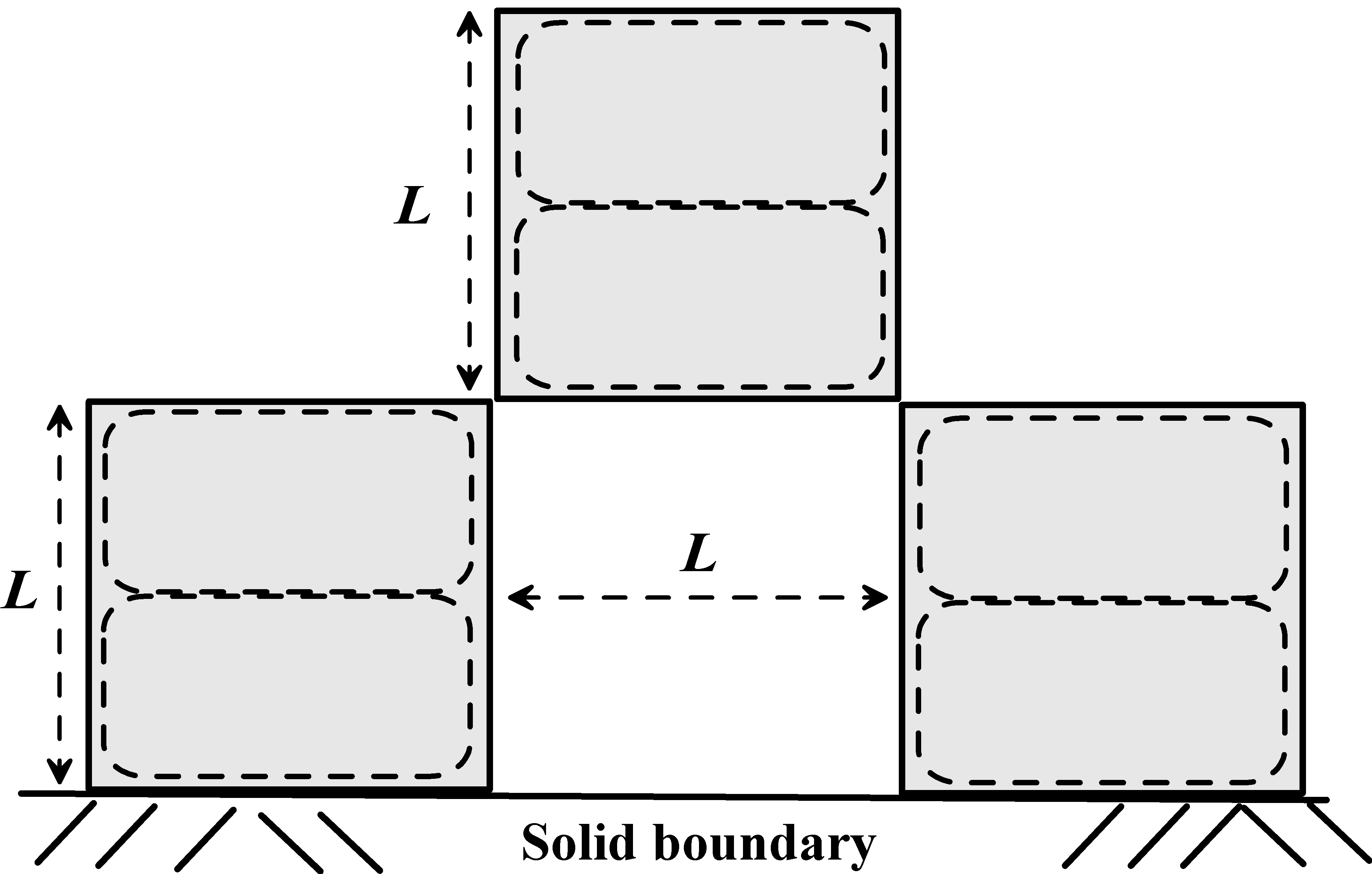
Figure 4: Squeezed vorticons like in the dark-grey square of Fig. 3. The dotted lines symbolize the circulation pattern within the squeezed quasi-particles.

7 Discussion

7.1 Kinetic theory and the $k$-$\omega$ closure of Wilcox

The specification $\zeta\equiv 1$ closes the primitive turbulence theory. In compact form it reads as follows:

$$\frac{\partial K}{\partial t}-\frac{\partial}{\partial\vec{x}}\left(\nu\,\frac{\partial K}{\partial\vec{x}}\right) = \nu\left(S^{2}-\Omega^{2}\right),$$ (65)

$$\frac{\partial\Omega}{\partial t}\;-\frac{\partial}{\partial\vec{x}}\left(\nu\,\frac{\partial\Omega}{\partial\vec{x}}\right) = \frac{1}{\pi}\left(\frac{1}{2}\,S^{2}-\Omega^{2}\right),$$ (66)

$$\nu = \frac{K}{\pi\,\Omega}\,.$$ (67)

These equations are structurally fully identical with the $k$-$\omega$ closure model discussed by Wilcox (2006) , which is in many aspects the best out of more than 10 other semi-empirical two-equation models. ‘His’ $k$ and our $K$ are equivalent. The eddy viscosity definitions of Wilcox and the present paper agree effectively up to a factor of ${\cal O}(1)$.

However, ‘his’ $\omega$ (he calls it somewhat uncertain a ‘specific dissipation rate’) differs significantly from our $\Omega$,

$$\omega=\Omega/\sqrt{\beta^{*}}\approx 3.3\bar{3}\cdot\Omega\,,$$ (68)

where $\beta^{*}=0.09$ is one out of 6 empirical parameters of the Wilcox model. It reproduces the logarithmic boundary layer and implies $\kappa=0.41$.

A major quantitative difference between the two models lays in the free homogenous decay. While both exhibit $K\sim t^{-m}$, we have $m=1$, which agrees with Dickey and Mellor’s (1980) high-$Re$ laboratory experiments and with Oberlack’s (2002) theoretical result for the free decay in the Navier-Stokes equation. Wilcox’ model is tuned to $m=6/5=1.2$, which agrees with a number of other laboratory results and with Oberlack’s (2002) result for the free decay in the Euler equation.

Today it is not clear why many decay experiments lead to $m>1$. Possibly it is a matter of initial conditions, see e.g. Hurst and Vassilicos (2007): at high $Re$ viscosity is comparatively small so that its regularizing effect on the initial spectrum towards a fully self-similar decay spectrum will take more time than at lower $Re$. In some cases this time may exceed the lifetime of turbulence.

7.2 Von Kármán’s number

The primitive theory makes a quantitative prediction of von Kármán’s constant. This allows a comparison with observations, experiments and competing other theories. While the latter are rare, there is a substantial literature discussing the precise value of $\kappa$ and its error bounds. The controversy whether the logarithmic or the power law is applicable to boundary layers (Barenblatt) shall not be picked up here. The controversy on the universality of $\kappa$ (Chauhan et al. 2005) is possibly only a matter of proper definition. If we restrict the definition of $\kappa$ to the case of $favorable$ pressure gradients only (cf. Chauhan et al.) then we would get a unique solution which is supported also by the Chauhan et al. data: $\kappa=0.40$.

A theoretical effort by Telford (1982) shall be mentioned, who derived a formula which connects $\kappa$ with two semi-empirical parameters, the entrainment and the decay constants. He predicts $\kappa=0.37$. Further theoretical work has been done by Yakhot and Orszag (1986) who found $\kappa=0.372$ based on renormalization-group approximations. Bergmann (1998) claimes that $\kappa=1/{\bf\it\bf e}\approx 0.368$, based on a new physical interpretation resting on semi-empirical considerations.

From an analysis of observational data Högström (1985) concludes $0.40\pm 0.01$, which is still accepted today among most practitioners. But Telford and Businger (1986) draw his analysis into question and underline the enormous methodical problems in connection with the evaluation of the experimental data.

Another group of authors supports the lower values, e.g. Jinyin et al. (2002). They report many different $\kappa$ values obtained in the past from different experiments and simulations, e.g. back to Nikuradse, Laufer, Lawn, Perry and Abell, Long et al., Millikan, and Zagarola and Smits (loc. cit. Jinyin et al.). They summarize that the lower and upper bounds of $\kappa$ are 0.36 and 0.45, respectively, whereby the range of experimental Reynolds numbers involved is also quite broad. In this sense Zanoun et al. (2003) support $\kappa=0.37$ while Nagib et al. (2004) prefer 0.38, underlining the influence of non-stationary conditions. Andreas et al. (2006) report a somewhat higher 0.387 $\pm\,0.003$ based on experimental material from the atmospheric boundary layer. However, in the Princeton superpipe a value of 0.421 has been found for smooth flow at $Re\approx 3\cdot 10^{7}$ (Smits 2007), too.

Summarizing the hot debates of the past, a review by Jimenez and Moser (2007) on wall turbulence states boldly: “The Kármán constant $\kappa\approx$ 0.4 is approximately universal.” In practice this can hardly be distinguished from our primitive-theoretical value 0.399 for $Re\rightarrow\infty$.

Nevertheless, doubts remain and the discussion by Talamelli et al. (2009) is justified. They underline the limitations of the various existing superpipe facilities and propose a new one that will allow good spatial resolution even at very high Reynolds number. The new facility is the international effort CICLoPE and under construction in North Italy.

7.3 Kinetic theory and spectra of turbulence

The above theory makes a precise prediction of von Kármán’s constant $\kappa$. Would it be possible to use the present kinetic picture of turbulence also to determine asymptotic values for the Kolmogorov constants $C_{K}$ and $C_{\omega}$ in the spectral energy distributions over frequency and wave number? With great probability the answer is no. Such an approach would demand that the lower bounds $\lambda_{u}$ and $\omega_{u}$ in the energy integrals could be specified:

$$K\;=\;C_{K}\,\varepsilon^{2/3}\int_{\lambda_{u}}^{\infty}k^{-5/3}\,dk\;=\;C_{\omega}\,\varepsilon\int_{\omega_{u}}^{\infty}\omega^{-2}\,d\omega\,.$$ (69)

These bounds are not simply connected with the ensemble-mean values of vorticity and length scale.

But it cannot be excluded that a dissipation theory of quasi-particles can be developed in analogy to a radioactive decay chain, where large quasi-particles are broken by a collision into smaller ones etc. down to the (infinitely small) Kolmogorov scale where they are annihilated. This could be imagined as a cup with a tiny whole. It would keep all quasi-particles of size $>0$ in and let only those out which have zero size. Possibly this approach could find some attention.

7.4 Conclusions

The primitive picture of turbulence makes a minimum use of the Navier-Stokes equation. Vortex properties are derived from the Euler equation and dissipaton is introduced through an analogy to a birth and death process. Methodically our position is a neighbor of Maxwell’s kinetic theory of real gases:

• Real gas: Free molecule flights and their collisions are strictly governed by inertia and short-range forces of a non-stationary Coulomb field with moving point sources. Maxwell neglected the details of these interactions. He replaced them with geometrical and probability considerations and a statistical equilibrium assumption. He got the probability distribution of the molecular energies whereby advective, rotational and potential energy of the molecules could be treated as statistically independent. In an isolated real gas total energy and molecule number are conservation quantities.

• Turbulence: Here neither energy nor particle number are conserved, but the flux of mechanical energy into a volume element is in quasi-equilibrium with the heat flux across the boundaries. In vortex dipoles translation and rotation are coupled and statistically $not$ independent. Nevertheless one may apply Maxwell’s central idea here as well. Although the movements of our quasi-particles are strictly governed by well-known rules (Navier and Stokes), we take them as unpredictable and replace them with geometry and probability arguments. Following Eward Lorenz (1960), such an approach stands today on much harder theoretical grounds than in Maxwell’s times.

We used only the following assumptions:

1. A turbulent fluid at $Re=\infty$ is a volume saturated with chaotically moving vortex-dipol tubes which are treated as quasi-particles.

2. A new-born quasi-particle is equipped with energy lost in from the mean flow formulated with the eddy-viscosity hypothesis, $-\langle u^{\prime}\,w^{\prime}\rangle=\nu\,S$. Its vorticity is governed by Tennekes’ hypothesis.

3. Advection of dipol tubes as quasi-particles follows simplest classical laws.

4. If quasi-particles collide they are either scattered (50 %) or annihilated/converted to heat (50 %).

5. If scattered they perform a Brownian motion with Einstein’s diffusivity in Prandtl-Kolmogorov formulation.

Acknowledgments. The author thanks Hartmut Peters in Seattle, Eckard Kleine in Hamburg and Michael Wilczek in Münster for their patience during turbulent discussions. He further thanks Rupert Klein in Berlin for still more patience, enduring interest, and substantial support.

References

- [Andeme(2008)] Andeme, R. A., 2008: Development of an oriented-eddy collision model for turbulence.. Ph.D. thesis, University of Massachusetts.
- [Andreas et al.(2006)Andreas, Claffey, Jordan, Fairall, Guest, Persson, and Grachev] Andreas, E. L., K. J. Claffey, R. E. Jordan, C. W. Fairall, P. S. Guest, P. O. G. Persson, and A. A. Grachev, 2006: Evaluation of the von-Kármán constant in the atmospheric boundary layer. J. Fluid Mech., 559, 117 – 149.
- [Aref(1983)] Aref, H., 1983: Integrable, chaotic and turbulent vortex motion in two-dimensional flows. Ann. Rev. Fluid Mech., 25, 345 – 389.
- [Barenblatt(1997)] Barenblatt, G. I., 1997: Scaling, self-similarity, and intermediate asymptotics.. Cambridge Texts in Applied Mathematics, Cambridge University Press, 386 pp.
- [Baumert(2005a)] Baumert, H. Z.: 2005a, A novel two-equation turbulence closure for high Reynolds numbers. Part B: Spatially non-uniform conditions. Marine Turbulence: Theories, Observations and Models, H. Z. Baumert, J. H. Simpson, and J. Sündermann, eds., Cambridge University Press, Chapter 4, 31 – 43.
- [Baumert(2005b)] — 2005b, On some analogies between high-Reynolds number turbulence and a vortex gas for a simple flow configuration. ibid. Chapter 5, 44 – 52.
- [Baumert and Peters(2004)] Baumert, H. Z. and H. Peters, 2004: Turbulence closure, steady state, and collapse into waves. J. Phys. Oceanography, 34, 505 – 512.
- [Bradshaw(1974)] Bradshaw, P., 1974: Possible origin of Prandt’s mixing-length theory. Nature, 249, 135 – 136.
- [Chauhan et al.(2005)Chauhan, Nagib, and Monkewitz] Chauhan, K. A., H. M. Nagib, and P. A. Monkewitz: 2005, Evidence on non-universality of Karman constant. Proc. iTi Conf. on Turbulence, 25 – 28 Sept, 4.
- [Chen et al.(2004)Chen, Orszag, Staroselsky, and Succi] Chen, H., S. Orszag, I. Staroselsky, and S. Succi, 2004: Expanded analogy between Boltzmann kinetic theory of fluids and turbulence. J. Fluid Mech., 519, 301 – 314.
- [Cottet and Koumoutsakos(2000)] Cottet, H.-H. and P. Koumoutsakos, 2000: Vortex Methods: Theory and Practice. Cambridge University Press, 311 pp.
- [Descartes(1644)] Descartes, R.: 1644, De mundo adspectabili. Principia philosophiae. Pars Tertia., A. L. Elzevirium, 334 pp., 70 – 190.
- [Dickey and Mellor(1980)] Dickey, T. D. and G. L. Mellor, 1980: Decaying turbulence in neutral and strati ed uids. J. Fluid Mech., 99, 37 – 48.
- [Eckhardt and Aref(1988)] Eckhardt, B. and H. Aref, 1988: Integrable and chaotic motions of four vortices II: collision dynamics of vortex pairs. Phil. Trans. R. Soc. Lond. A, 326, 655 – 696.
- [Einstein(1905)] Einstein, A., 1905: Über die von der molekularkinetischen Theorie der Wärme geforderte Bewegung von in ruhenden Fl ssigkeiten suspendierten Teilchen. Annalen der Physik, 17, 549 – 560.
- [Falkovich and Sreenivasan(2006)] Falkovich, G. and K. Sreenivasan, 2006: Lessons from hydrodynamic turbulence. Physics Today, 43 – 49.
- [Frenzen and Vogel(1994)] Frenzen, P. and C. A. Vogel, 1994: On the magnitude and apparent range of variation of the von Karman constant in the atmospheric surface layer. Boundary-Layer Meteorology, 72, 371 – 392.
- [Frisch(1995)] Frisch, U., 1995: Turbulence - the Legacy of A. N. Kolmogorov. Cambridge University Press, Cambridge, MA, 296 pp.
- [Haken(1978)] Haken, H., 1978: Synergetics. Springer-Verlag, 2 edition, 355 pp.
- [Haken(1983)] — 1983: Advanced Synergetics. Springer-Verlag, 355 pp.
- [Högström(1985)] Högström, U., 1985: Von Kármán’s constant in atmospheric boundary layer flow: reevaluated. J. Atmos. Sci., 42, 263 – 270.
- [Hurst and Vassilicos(2007)] Hurst, D. and J. C. Vassilicos, 2007: Scaling and decay of fractal-generated turbulence. Physics of Fluids, 19, 035103.1 – 035103.31.
- [Jimenez and Moser(2007)] Jimenez, J. and R. D. Moser, 2007: What are we learning from simulating wall turbulence? Phil. Trans. R. Soc. A, 365, 715 – 732.
- [Jinyin et al.(2002)Jinyin, Maozhao, and Durst] Jinyin, Z., X. Maozhao, and F. Durst, 2002: On the effect of Reynolds number on von Karman’s constant. Acta Mechanica Sinica (English Series), 18, 350 – 355.
- [Keller and Fridman(1924)] Keller, L. W. and A. A. Fridman: 1924, Differentialgleichung für die turbulente Bewegung einer kompressiblen Flüssigkeit. Proc. 1st Int. Congr. Appl. Mech., C. Biezeno and J. Burgers, eds., Technische Boekhandel en Drukkerij J. Waltman Jr., 22 – 24 April, 395 – 405.
- [Klein and Majda(1993)] Klein, R. and A. Majda, 1993: An asymptotic theory for the nonlinear instability of antiparallel pairs of vortex filaments. Phys. Fluids A, 5, 369 – 379.
- [Kolmogorov(1941)] Kolmogorov, A. N., 1941: The local structure of turbulence in incompressible viscous fluids for very large Reynolds numbers. Dokl. Akad. Nauk SSSR, 30, 299 – 302.
- [Kundu(1990)] Kundu, P. K., 1990: Fluid Mechanics. Academic Press, 638 pp.
- [Lamb(1932)] Lamb, H., 1932: Hydrodynamics. Cambridge University Press, 6 edition, 738 pp.
- [Lesieur(1997)] Lesieur, M., 1997: Turbulence in Fluids.. Kluwer Ac. Publ., 3 edition, 515 pp.
- [Lions and Majda(2000)] Lions, P.-L. and A. Majda, 2000: Equilibrium statistical theory for nearly parallel vortex filaments. Comm. Pure Appl. Math., Vol. LIII, 76 – 142.
- [Lorenz(1960)] Lorenz, E. N., 1960: Maximum simplification of the dynamic equations. Tellus, 12, 243 – 254.
- [Marmanis(1998)] Marmanis, H., 1998: The kinetic theory of point vortices. Proc. R. Soc. London A, 454, 587 – 606.
- [Maxwell(1867)] Maxwell, J. C., 1867: On the dynamic theory of gases. Phil. Trans. R. Soc. London, 157, 49 – 88.
- [Nagib et al.(2004)Nagib, Christophorou, and Monkewitz] Nagib, H., C. Christophorou, and P. Monkewitz: 2004, Impact of pressure-gradient conditions on high Reynolds number turbulent boundary layers. Abstracts Proc. XXI ICTAM, 15-21 August 2004, 2.
- [Oberlack(2002)] Oberlack, M., 2002: On the decay exponent of isotropic turbulence. Proc. Appl. Math. Mech. (PAMM), 1, 294 – 297.
- [Onsager(1949)] Onsager, L., 1949: Statistical hydrodynamics. Nuovo Cimento, 6, (Suppl.), 279 – 287.
- [Prandtl(1925)] Prandtl, L., 1925: Bericht über Untersuchungen zur ausgebildeten Turbulenz. Ztschr. angew. Math. Mech. (ZAMM), 5, 136 – 139.
- [Reynolds(1895)] Reynolds, O., 1895: On the dynamical theory of incompressible viscous fluids and the determination of the criterion. Phil. Trans. R. Soc. London A, 186, 123 – 164.
- [Saffman(1992)] Saffman, P.-G., 1992: Vortex Dynamics.. Cambridge University Press, 308 pp.
- [Schlichting and Gersten(2000)] Schlichting, H. and K. Gersten, 2000: Boundary Layers. Springer, 799 pp.
- [Smits(2007)] Smits, A.: 2007, Turbulence in Pipes: The Moody Diagram and Moore Moore s Law. Proc. ASME Fluids Engineering Conference, 57.
- [Telford(1982)] Telford, J. W., 1982: A theoretical value for von Karman’s constant. Pure and Appl. Geophysics, 120, 648 – 661.
- [Telford and Businger(1986)] Telford, J. W. and J. A. Businger, 1986: Comments on ‘Von Kármán’s constant in atmospheric boundary layer flow: reevaluated.’. J. Atmos. Sci., 43, 2127 – 2130.
- [Vinen and Donnelly(2007)] Vinen, W. F. and R. J. Donnelly, 2007: Quantum turbulence. Physics Today, 43 – 48.
- [Wilcox(2006)] Wilcox, D. C., 2006: Turbulence Modeling for CFD. DCW Industries, Inc., 3rd edition, 522 pp.
- [Yakhot and Orszag(1986)] Yakhot, V. and S. A. Orszag, 1986: Renormalization-group analysis of turbulence. Phys. Rev. Lett., 57, 1722 – 1724.
- [Zanoun et al.(2003)Zanoun, Durst, and Nagib] Zanoun, E. S., F. Durst, and H. Nagib, 2003: Evaluating the law of the wall in two-dimensional fully developed turbulent channel. Phys. Fluids, 15, 1 – 11.