$K\pi$ form factors and final state interactions in $D^{+}\to K^{-}\pi^{+}\pi^{+}$ decays

Abstract

We present a model for the decay $D^{+}\to K^{-}\pi^{+}\pi^{+}$. The weak interaction part of this reaction is described using the effective weak Hamiltonian in the factorisation approach. Hadronic final state interactions are taken into account through the $K\pi$ scalar and vector form factors fulfilling analyticity, unitarity and chiral symmetry constraints. The model has only two free parameters that are fixed from experimental branching ratios. We show that the modulus and phase of the $S$ wave thus obtained agree nicely with experiment up to 1.55 GeV. We perform Monte Carlo simulations to compare the predicted Dalitz plot with experimental analyses. Allowing for a global phase difference between the $S$ and $P$ waves of $-65^{\circ}$, the Dalitz plot of the $D^{+}\to K^{-}\pi^{+}\pi^{+}$ decay, the $K\pi$ invariant mass spectra and the total branching ratio due to $S$-wave interactions are well reproduced.

I Introduction

In 2002, the analysis of $D^{+}\to K^{-}\pi^{+}\pi^{+}$ decays performed by the E791 collaboration revealed that approximately 50% of these decays proceed through a low-mass scalar resonance with isospin $1/2$: the $K_{0}^{*}(800)$, also called the $\kappa$ Aitala:2002kr . As a matter of fact, the $\kappa$ was the second elusive scalar to be firmly detected in $D^{+}$ decays since the scalar-isoscalar $f_{0}(600)$, or $\sigma$, had been detected by the same collaboration in $D^{+}\to\pi^{+}\pi^{-}\pi^{+}$ E791sigma . More recently, the $D^{+}\to K^{-}\pi^{+}\pi^{+}$ decay was revisited by E791 Aitala:2005yh and two other experiments produced analyses based on larger data samples, namely FOCUS Pennington:2007se ; Focus2009 and CLEO Bonvicini:2008jw . The main conclusions of the pioneering E791 work have been confirmed in both cases.

In the past, many analyses of $K\pi$ scattering data had already claimed the presence of the $\kappa$ pole in the scattering amplitude kappapoles1 ; kappapoles2 ; kappapoles3 ; JOPscatt . The most precise and model independent determination of its position in the second Riemann sheet was produced in Ref. MoussallamKappa , following the method put forward for the $\sigma$ in Ref. CCL . Using Roy’s equations for $K\pi$ scattering Roy and Chiral Perturbation Theory (ChPT) ChPT Descotes-Genon and Moussallam found $m_{\kappa}=658\pm 13$ MeV and $\Gamma_{\kappa}=557\pm 24$ MeV MoussallamKappa .

Although the experimental results are sound and the $\kappa$ pole is at present theoretically well known, a comprehensive and successful description of the reaction $D^{+}\to K^{-}\pi^{+}\pi^{+}$ is still not available (for a recent review see Ref. Reviews ). Experimentalists, for the want of a better framework, commonly fit their data with the isobar model which consists of a weighted sum of Breit-Wigner-like propagators. Often, a complex constant is added to the amplitude in order to account for the non-resonant decays. It is known, nevertheless, that the adoption of Breit-Wigner functions to describe the effect of scalar resonances is problematic. Some of the deficiencies of this approach are discussed in Ref. Oller:2004xm where Oller proposed the substitution of these functions in the $S$ wave by expressions based on unitarised ChPT UniChPT . This model provides a good description of the data but, since the weak part of the decay was not tackled, the relative weight of the amplitudes remain arbitrary complex parameters to be determined from the fit.

Little progress has been achieved in the treatment of weak decays of charmed mesons since the seminal papers by Bauer, Stech and Wirbel Wirbel:1985ji ; Bauer:1986bm . This fact stems from the mass of the $c$-quark that lies between the heavy and the light domains, rendering heavy-quark approaches or the use of chiral symmetry less trustworthy. A first attempt to describe the decay $D^{+}\to K^{-}\pi^{+}\pi^{+}$ from first principles was made by Diakonou and Diakonos in Ref. Diakonou:1989sf . In their work, the weak amplitude was described within naïve factorisation with the weak Hamiltonian of Refs. Wirbel:1985ji ; Bauer:1986bm and the final state interactions (FSIs) were implemented by means of Breit-Wigner type $K\pi$ form factors. They considered the contribution of two resonances, namely the $K^{*}(892)$ and the $K_{0}^{*}(1430)$. In the light of the present empirical data it is clear that this model cannot provide a good description of the decay. In Ref. Diakonou:1989sf , the decay is mainly driven by the $K^{*}(892)$ whereas the analyses of Refs. Aitala:2002kr ; Aitala:2005yh ; Pennington:2007se ; Focus2009 ; Bonvicini:2008jw show that the decay is largely dominated by $K\pi$ pairs in an $S$-wave state. On average, the total scalar signal amounts to 82% Amsler:2008zzb . Hence, a more comprehensive model for the whole scalar contribution is needed to provide a good description of the data. A first step in this direction was taken in Refs. Gardner:2001gc ; Gardner2 where the $\pi\pi$ scalar signal in $B\to\pi\pi\pi$ decays was considered. In this framework, factorisation is assumed for the weak amplitude and the $\pi\pi$ scalar form factor, constrained by chiral dynamics and unitarity, provides the description of FSIs Meissner:2000bc . In Refs. Furman:2005xp ; ElBennich:2006yi , a similar description was utilised to describe the $S$ wave in $B\to\pi\pi K$ and $B\to K\bar{K}K$ decays. Using the same method, $S$-wave FSIs have also been considered in the decay $D^{+}\to\pi^{+}\pi^{-}\pi^{+}$ Boito:2008zk . More recently, $K\pi$ form factors have been employed in the description of FSIs in $B^{\pm}\to K^{\pm}\pi^{\mp}\pi^{\pm}$ decays BenoitBKpipi . In the present work, we follow the same general scheme where a factorised weak decay amplitude is dressed with FSIs by means of non-perturbative $K\pi$ form factors.

For the weak vertex, we employ the effective weak Hamiltonian of Refs. Wirbel:1985ji ; Bauer:1986bm within naïve factorisation. Although the assumption of factorisation is less reliable for the $c$-quark mass scale, it has been successfully applied to $D$ decays in several recent papers Boito:2008zk ; Bediaga:1996ue ; Bediagaetal2 ; Rosenfeld ; Cheng:2002ai ; f0 . However, one should consider the Wilson coefficients as phenomenological parameters to compensate for the deficiencies of factorisation Buras:1994ij . The phenomenological values are close to the calculated ones Heff but have larger errors than in applications to $B$ decays. The weak amplitude thus obtained receives contributions from colour-allowed and colour-suppressed topologies. In the latter, the $K\pi$ form factors appear manifestly and the construction of the final state is straightforward. The colour-allowed topology is more involved but, assuming the decay to be mediated by resonances as suggested by the experimental results, the FSIs in this case can also be written in terms of $K\pi$ form factors Gardner:2001gc ; Boito:2008zk . Therefore, in our description the hadronic FSIs are fully taken into account by the $K\pi$ scalar and vector form factors.

Both form factors have received attention in recent years and are now well known in the energy regime relevant to $D^{+}\to K^{-}\pi^{+}\pi^{+}$ decays. The scalar component was studied in a framework that incorporates all the known theoretical constraints in Refs. Jamin:2001zq ; JOP2 ; JOP3 . Analyticity, unitarity, chiral symmetry, the large-$N_{c}$ limit of QCD, and the coupling to $K\eta$ and $K\eta^{\prime}$ channels were taken into account. The results were subsequently updated and we employ in this work the state-of-the-art version given in Ref. Jamin:2006tj . The vector form factor, in its turn, can be studied in $\tau^{-}\to K\pi\nu_{\tau}$ decays Jamin:2006tk ; JPP2 ; Moussallam ; Boito:2008fq , where the kinematical range is very similar to the one considered in this paper. A prediction for this form factor within Resonance Chiral Theory (RChT) RChT was presented in Ref. Jamin:2006tk and, after the appearance of the detailed spectrum measured by the Belle collaboration Belle , a fit was performed in Ref. JPP2 . Here we employ a slightly different description which fulfils analyticity constraints and that was successfully fitted to the Belle spectrum in Ref. Boito:2008fq .

Our paper is organised as follows. In Section II we present our model and discuss previous treatments of the same decay found in the literature. The numerical results are worked out in Section III. Finally, we give a summary and discuss the results in Section IV. Details about the construction of the $K\pi$ form factors employed in this work are relegated to the Appendix.

II Theoretical framework

Our phenomenological description of the weak process $D^{+}\to K^{-}\pi^{+}\pi^{+}$ is based on the effective Hamiltonian

$${\cal H}_{\rm eff}=\frac{G_{F}}{\sqrt{2}}V_{cs}V_{ud}^{\ast}[C_{1}(\mu)O_{1}+C_{2}(\mu)O_{2}]+\mbox{h.c.}\ ,$$ (1)

where $G_{F}=1.16637\times 10^{-5}\ \mbox{GeV}^{-2}$ is the Fermi decay constant Amsler:2008zzb , $V_{cs}V_{ud}^{\ast}=1-\lambda^{2}$, in the Wolfenstein parametrisation Wolfenstein:1983yz with $\lambda\equiv\sin\theta_{C}=0.2257$ Amsler:2008zzb , $C_{1,2}(\mu)$ are short distance Wilson coefficients computed at the renormalisation scale $\mu={\cal O}(m_{c})$, and $O_{1,2}$ are the local four-quark operators

$$\begin{array}[]{c}O_{1}=[\bar{c}_{i}\gamma^{\mu}(1-\gamma_{5})s_{i}][\bar{d}_{j}\gamma_{\mu}(1-\gamma_{5})u_{j}]\ ,\\ O_{2}=[\bar{c}_{i}\gamma^{\mu}(1-\gamma_{5})s_{j}][\bar{d}_{j}\gamma_{\mu}(1-\gamma_{5})u_{i}]\ ,\end{array}$$ (2)

with $(i,j=1,2,3)$ denoting colour indices. At the quark level, the decay $D^{+}\to K^{-}\pi^{+}\pi^{+}$ is driven by the transition $c\to su\bar{d}$, i.e. four different quark flavours are involved. In this case, only the two tree operators in Eq. (2) have to be taken into account.

The amplitude for $D^{+}\to K^{-}\pi^{+}\pi^{+}$ is given by the matrix element $\langle K^{-}\pi^{+}\pi^{+}|{\cal H}_{\rm eff}|D^{+}\rangle$. We assume the factorisation approach to hold at leading order (in $\Lambda_{\rm QCD}/m_{c}$ and $\alpha_{s}$) and as a consequence the amplitude is written in terms of colour allowed and suppressed contributions, ${\cal A}_{1}$ and ${\cal A}_{2}$ respectively, as

$${\begin{array}[]{rcl}{\cal A}(D^{+}\to K^{-}\pi^{+}\pi^{+})&=&\displaystyle\frac{G_{F}}{\sqrt{2}}\cos^{2}\theta_{C}(a_{1}{\cal A}_{1}+a_{2}{\cal A}_{2})+(\pi^{+}_{1}\leftrightarrow\pi^{+}_{2})\\[8.61108pt] &=&\displaystyle\frac{G_{F}}{\sqrt{2}}\cos^{2}\theta_{C}[a_{1}\langle K^{-}\pi^{+}_{1}|\bar{s}\gamma^{\mu}(1-\gamma_{5})c|D^{+}\rangle\langle\pi^{+}_{2}|\bar{u}\gamma_{\mu}(1-\gamma_{5})d|0\rangle\\[8.61108pt] &&+a_{2}\langle K^{-}\pi^{+}_{1}|\bar{s}\gamma^{\mu}(1-\gamma_{5})d|0\rangle\langle\pi^{+}_{2}|\bar{u}\gamma_{\mu}(1-\gamma_{5})c|D^{+}\rangle]+(\pi^{+}_{1}\leftrightarrow\pi^{+}_{2})\ ,\end{array}}$$ (3)

where the last term accounts for the presence of two identical pions in the final state. The QCD factors $a_{1,2}(\mu)$ are related to $C_{1,2}(\mu)$ as follows:

$$a_{1}(\mu)=C_{1}(\mu)+\frac{1}{N_{c}}C_{2}(\mu)\ ,\quad a_{2}(\mu)=C_{2}(\mu)+\frac{1}{N_{c}}C_{1}(\mu)\ ,$$ (4)

where $N_{c}=3$ is the number of colours. For these factors we use the phenomenological values

$$a_{1}=1.2\pm 0.1\ ,\qquad a_{2}=-0.5\pm 0.1\ ,$$ (5)

obtained from different analyses of two-body $D$ meson decays Buras:1994ij .

The non-perturbative hadronic matrix elements in Eq. (3) involve several Lorentz invariant form factors. We first consider those related to the ${\cal A}_{2}$ contribution. The transition $D^{+}\to K^{-}\pi^{+}$ appearing in ${\cal A}_{1}$ is more involved and requires a separate analysis. The matrix element from the vacuum to the $K\pi$ final state is given by

$$\langle K^{-}\pi^{+}_{1}|\bar{s}\gamma^{\mu}d|0\rangle=\left[(p_{K}-p_{\pi_{1}})^{\mu}-\frac{m_{K}^{2}-m_{\pi}^{2}}{q^{2}}q^{\mu}\right]F_{+}^{K\pi}(q^{2})+\frac{m_{K}^{2}-m_{\pi}^{2}}{q^{2}}q^{\mu}F_{0}^{K\pi}(q^{2})\ ,$$ (6)

where $q=p_{K}+p_{\pi_{1}}$ and $F_{+,0}^{K\pi}(q^{2})$ are the $K\pi$ vector and scalar form factors. Analogously, the transition $D^{+}\to\pi^{+}$ is given by

$$\langle\pi^{+}_{2}|\bar{u}\gamma^{\mu}c|D^{+}\rangle=\left[(p_{D}+p_{\pi_{2}})^{\mu}-\frac{m_{D}^{2}-m_{\pi}^{2}}{q^{2}}q^{\mu}\right]F_{+}^{D\pi}(q^{2})+\frac{m_{D}^{2}-m_{\pi}^{2}}{q^{2}}q^{\mu}F_{0}^{D\pi}(q^{2})\ ,$$ (7)

where now $q=p_{D}-p_{\pi_{2}}$ and $F_{+,0}^{D\pi}(q^{2})$ are the $D\pi$ vector and scalar transition form factors, respectively. The amplitude ${\cal A}_{2}$ then reads

$${\begin{array}[]{rcl}{\cal A}_{2}&=&\left[m_{K\pi_{2}}^{2}-m_{\pi_{1}\pi_{2}}^{2}-\displaystyle\frac{(m_{K}^{2}-m_{\pi}^{2})(m_{D}^{2}-m_{\pi}^{2})}{m_{K\pi_{1}}^{2}}\right]F_{+}^{K\pi}(m_{K\pi_{1}}^{2})F_{+}^{D\pi}(m_{K\pi_{1}}^{2})\\[8.61108pt] &&+\displaystyle\frac{(m_{K}^{2}-m_{\pi}^{2})(m_{D}^{2}-m_{\pi}^{2})}{m_{K\pi_{1}}^{2}}F_{0}^{K\pi}(m_{K\pi_{1}}^{2})F_{0}^{D\pi}(m_{K\pi_{1}}^{2})\ ,\end{array}}$$ (8)

where the Mandelstam variables are defined as

$$m_{K\pi_{1}}^{2}\equiv(p_{K}+p_{\pi_{1}})^{2}\ ,\qquad m_{K\pi_{2}}^{2}\equiv(p_{K}+p_{\pi_{2}})^{2}\ ,\qquad m_{\pi_{1}\pi_{2}}^{2}\equiv(p_{\pi_{1}}+p_{\pi_{2}})^{2}\ ,$$ (9)

with $m_{K\pi_{1}}^{2}+m_{K\pi_{2}}^{2}+m_{\pi_{1}\pi_{2}}^{2}=m_{D}^{2}+m_{K}^{2}+2m_{\pi}^{2}$.

In our analysis, we use a simple pole prescription for the $D\pi$ transition form factors,

$$F_{+,0}^{D\pi}(q^{2})=\frac{F_{+,0}^{D\pi}(0)}{1-q^{2}/m_{\rm pole}^{2}}\ ,$$ (10)

with $m_{\rm pole}=m_{D^{\ast 0}}$ for the vector case and $m_{\rm pole}=m_{D^{\ast 0}_{0}}$ for the scalar one. The normalisation constant is by construction the same in both cases $F_{+}^{D\pi}(0)=F_{0}^{D\pi}(0)$. This parametrisation agrees with experiment. The analysis performed by the Belle Coll. on $D^{0}\to\pi^{-}l^{+}\nu$ data gives for the simple pole model $m_{\rm pole}(1^{--})=1.97\pm 0.09$ Widhalm:2006wz , which is compatible with the PDG value $m_{D^{\ast\pm}}=2.01\ \mbox{GeV}$ Amsler:2008zzb . Then, in Eq. (10) we take $F_{+}^{D\pi}(0)=0.624$ from Ref. Widhalm:2006wz and $m_{D^{\ast 0}}=2007\ \mbox{MeV}$ and $m_{D^{\ast 0}_{0}}=2.352\pm 0.050\ \mbox{GeV}$ from Ref. Amsler:2008zzb .

For the $K\pi$ vector and scalar form factors, we employ the same expressions that were used in the successful reanalysis of $\tau^{-}\to K\pi\nu_{\tau}$ decays performed in Ref. Boito:2008fq . Since the kinematical region for the $K\pi$ system available in $D\to K\pi\pi$ decays, $m_{K}+m_{\pi}\leq m_{K\pi}\leq m_{D}-m_{\pi}$, is very similar to that of $\tau^{-}\to K\pi\nu_{\tau}$ decays, $m_{K}+m_{\pi}\leq m_{K\pi}\leq m_{\tau}$, we consider this choice appropriate. Both form factors are constructed such that they fulfil constraints posed by analyticity and unitarity. Because of these properties, the form factors satisfy an $n$-subtracted dispersion relation, which in the elastic region admit the well-known Omnès solution Omnes:1958hv . For the $K\pi$ vector form factor $F_{+}^{K\pi}(s)$, a good description of the experimental measurement of $\tau^{-}\to K\pi\nu_{\tau}$ was achieved by incorporating two vector resonances and working with a three-times-subtracted dispersion relation in order to suppress higher-energy contributions Boito:2008fq . The additionally required scalar $K\pi$ form factor $F_{0}^{K\pi}(s)$ had been calculated in the framework of RChT and solving dispersion relations for a three-body coupled-channel problem in Ref. Jamin:2001zq . Here, we use the recent numerical update of Ref. Jamin:2006tj . The details of the form factors used in this work can be found in Appendix A.

Now, we turn our attention to the form factors associated with the ${\cal A}_{1}$ contribution. The form factor denoting the transition from the vacuum to a pion final state is nothing else than

$$\langle\pi^{+}_{2}|\bar{u}\gamma_{\mu}(1-\gamma_{5})d|0\rangle=ifp_{\pi_{2}}\ ,$$ (11)

where the constant $f$ equals at lowest order in the chiral expansion the pion decay constant $f=f_{\pi}=\sqrt{2}F_{\pi}=130.5$ MeV. The form factors related to the transition $D^{+}\to K^{-}\pi^{+}$ are more complicated. On general grounds, the matrix element $\langle K^{-}\pi^{+}_{1}|\bar{s}\gamma^{\mu}(1-\gamma_{5})c|D^{+}\rangle$ can be written in terms of four different form factors Kuhn:1992nz . But, when saturated with $\langle\pi^{+}_{2}|\bar{u}\gamma_{\mu}(1-\gamma_{5})d|0\rangle$ only one of those form factors survives, $F_{4}$, and the amplitude ${\cal A}_{1}$ becomes

$${\cal A}_{1}=-if_{\pi}m_{\pi}^{2}F_{4}(m_{K\pi_{1}}^{2},m_{K\pi_{2}}^{2})\ .$$ (12)

Since this amplitude is proportional to $m_{\pi}^{2}$ one would expect it is negligible, as presumed in Ref. Bediaga:1996ue . If this were the case, however, the decay $D^{+}\to K^{-}\pi^{+}\pi^{+}$ would be dominated by the $P$-wave contribution (as demonstrated in Table 3 of Section III) in contradiction with experiment Amsler:2008zzb . This fact forces one to consider the ${\cal A}_{1}$ contribution in detail. Unfortunately, the contribution of $F_{4}$ to semileptonic decays, $D^{+}\to K^{-}\pi^{+}l^{+}\nu_{l}$ ($l=e,\mu$), is proportional to the lepton masses and neglected Bajc:1997nx . Consequently, one has to resort to theoretical models.

Several methods have been considered in the literature. Most of them are based on the assumption that the $D^{+}\to K^{-}\pi^{+}$ transition is driven by intermediate resonances, mainly vectors and scalars in this case. We will not take into account the contribution of tensor resonances. In the simplest case, one can consider the exchange of a single vector and scalar resonance using a Breit-Wigner parametrisation. For instance, in the paper by Diakonou and Diakonos Diakonou:1989sf the colour allowed contribution is written via the exchange of $K^{\ast}(892)$ and $K^{\ast}_{0}(1430)$ resonances as

$${\begin{array}[]{rcl}{\cal A}_{1}&=&\left[\displaystyle\sum_{\rm pol}\frac{\langle K^{-}\pi_{1}^{+}|\bar{K}^{\ast}\rangle\langle\bar{K}^{\ast}|\bar{s}\gamma^{\mu}(1-\gamma_{5})c|D^{+}\rangle}{m_{\bar{K}^{\ast}}^{2}-m_{K\pi_{1}}^{2}}+\frac{\langle K^{-}\pi_{1}^{+}|\bar{K}^{\ast}_{0}\rangle\langle\bar{K}^{\ast}_{0}|\bar{s}\gamma^{\mu}(1-\gamma_{5})c|D^{+}\rangle}{m_{\bar{K}^{\ast}_{0}}^{2}-m_{K\pi_{1}}^{2}}\right]\\[8.61108pt] &&\times\langle\pi^{+}_{2}|\bar{u}\gamma_{\mu}(1-\gamma_{5})d|0\rangle\ ,\end{array}}$$ (13)

while the colour suppressed contribution is given by Eq. (8) but with monopole $K\pi$ form factors, $F_{+,0}^{K\pi}(q^{2})=F_{+,0}^{K\pi}(0)/(1-q^{2}/m_{\rm pole}^{2})$, with $m_{\rm pole}=m_{\bar{K}^{\ast}(892)}$ for the vector and $m_{\rm pole}=m_{\bar{K}^{\ast}_{0}(1430)}$ for the scalar. Taking the matrix elements from Refs. Wirbel:1985ji ; Bauer:1986bm one gets

$${\cal A}_{1}=\frac{f_{\pi}g_{\bar{K}^{\ast}K\pi}m_{\bar{K}^{\ast}}N(m_{\bar{K}^{\ast}}^{2})F_{+}^{D\bar{K}^{\ast}}(m_{\pi}^{2})}{m_{\bar{K}^{\ast}}^{2}-m_{K\pi_{1}}^{2}-im_{\bar{K}^{\ast}}\Gamma_{\bar{K}^{\ast}}}+\frac{f_{\pi}g_{\bar{K}^{\ast}_{0}K\pi}m_{\bar{K}^{\ast}_{0}}(m_{D}^{2}-m_{\bar{K}^{\ast}_{0}}^{2})F_{0}^{D\bar{K}^{\ast}_{0}}(m_{\pi}^{2})}{m_{\bar{K}^{\ast}_{0}}^{2}-m_{K\pi_{1}}^{2}-im_{\bar{K}^{\ast}_{0}}\Gamma_{\bar{K}^{\ast}_{0}}}\ ,$$ (14)

where $N(q^{2})=m_{D}^{2}+m_{K}^{2}+2m_{\pi}^{2}-2m_{\pi_{1}\pi_{2}}^{2}-q^{2}-M(q^{2})$, $M(q^{2})=(m_{K}^{2}-m_{\pi}^{2})(m_{D}^{2}-m_{\pi}^{2})/q^{2}$, $g_{\bar{K}^{\ast}K\pi}(g_{\bar{K}^{\ast}_{0}K\pi})$ are dimensionless couplings associated to $\langle K^{-}\pi_{1}^{+}|\bar{K}^{\ast}(\bar{K}^{\ast}_{0})\rangle$, and $F_{+}^{D\bar{K}^{\ast}}(m_{\pi}^{2})$ and $F_{0}^{D\bar{K}^{\ast}_{0}}(m_{\pi}^{2})$ are pertinent vector and scalar transition form factors evaluated at $q^{2}=m_{\pi}^{2}$. Again, a monopole form is assumed,

$$F_{+}^{D\bar{K}^{\ast}}(q^{2})=\frac{F_{+}^{D\bar{K}^{\ast}}(0)}{1-q^{2}/m_{\rm pole}^{2}}\ ,\qquad F_{0}^{D\bar{K}^{\ast}_{0}}(q^{2})=\frac{F_{0}^{D\bar{K}^{\ast}_{0}}(0)}{1-q^{2}/m_{\rm pole}^{2}}\ ,$$ (15)

with $m_{\rm pole}=m_{D_{s}^{\pm}}$ in both cases Wirbel:1985ji ; Bauer:1986bm .

Experimental data collected in Tables 1 and 2 indicate that the vector contribution to the total signal is largely dominated by the exchange of $K^{\ast}(892)$. Hence, a Breit-Wigner parametrisation with a single vector resonance, as considered in Ref. Diakonou:1989sf , should be a reasonable approximation to the vector induced signal. This is not the case for the scalar one, where the contribution of $K^{\ast}_{0}(1430)$ is marginal. Besides, the possible $K^{\ast}_{0}(800)$ or $\kappa$ and non-resonant contributions are not accounted for in Eq. (14). Therefore, a more elaborated prescription taking into account the whole scalar contribution is mandatory. Here, we follow Ref. Gardner:2001gc and write the colour allowed amplitude ${\cal A}_{1}$ in terms of the scalar and vector $K\pi$ form factors. We briefly summarise the method applied to our case. The $D^{+}\to K^{-}\pi^{+}$ matrix element is written as

$$\langle K^{-}\pi^{+}|\bar{s}\gamma^{\mu}(1-\gamma_{5})c|D^{+}\rangle=\sum_{R=S,V}\langle K^{-}\pi^{+}|R\rangle P_{R}\langle R|\bar{s}\gamma^{\mu}(1-\gamma_{5})c|D^{+}\rangle\ ,$$ (16)

where we assumed that only scalar and vector intermediate resonances propagate. Tensor resonances are not included in the sum since the $K_{2}^{\ast}(1430)$ is seen to contribute less than 1% Amsler:2008zzb . In Eq. (16), $\langle K^{-}\pi^{+}|R\rangle$ is the coupling of $K\pi$ to the resonance and $P_{R}$ stands for the propagation of that resonance. The same decomposition is possible for the matrix element which define the scalar and vector form factors. Our aim is to substitute the products $\langle K^{-}\pi^{+}|R\rangle P_{R}$, usually involving Breit-Wigner parametrisations, by expressions based on the relevant form factors.

For the scalar case, let us take for instance the contribution of $K^{\ast}_{0}(1430)$ alone and write

$$\langle K^{-}\pi^{+}|\bar{s}d|0\rangle=\frac{m_{K}^{2}-m_{\pi}^{2}}{m_{s}-m_{d}}F_{0}^{K\pi}(q^{2})=\langle K^{-}\pi^{+}|\bar{K}^{\ast}_{0}\rangle P_{\bar{K}^{\ast}_{0}}(q^{2})\langle\bar{K}^{\ast}_{0}|\bar{s}d|0\rangle\ ,$$ (17)

where the matrix element $\langle\bar{K}^{\ast}_{0}|\bar{s}d|0\rangle$ defines the scalar decay constant. Then,

$$\Pi_{\bar{K}^{\ast}_{0}K\pi}(q^{2})\equiv\langle K^{-}\pi^{+}|\bar{K}^{\ast}_{0}\rangle P_{\bar{K}^{\ast}_{0}}(q^{2})=\frac{1}{\langle\bar{K}^{\ast}_{0}|\bar{s}d|0\rangle}\frac{m_{K}^{2}-m_{\pi}^{2}}{m_{s}-m_{d}}F_{0}^{K\pi}(q^{2})\equiv\chi_{\bar{K}^{\ast}_{0}}F_{0}^{K\pi}(q^{2})\ ,$$ (18)

with $\chi_{\bar{K}^{\ast}_{0}}$ a pure number understood as a normalisation. Hence, the contribution to the matrix element in Eq. (16) is

$$\langle K^{-}\pi^{+}|\bar{s}\gamma^{\mu}(1-\gamma_{5})c|D^{+}\rangle\Big{|}_{\bar{K}^{\ast}_{0}}=\chi_{\bar{K}^{\ast}_{0}}F_{0}^{K\pi}(q^{2})\langle\bar{K}^{\ast}_{0}|\bar{s}\gamma^{\mu}(1-\gamma_{5})c|D^{+}\rangle\ .$$ (19)

In order to make contact with Ref. Diakonou:1989sf one can consider the function $\Pi_{\bar{K}^{\ast}_{0}K\pi}$ in a Breit-Wigner parametrisation,

$$\Pi_{\bar{K}^{\ast}_{0}K\pi}^{\rm BW}(q^{2})=\frac{g_{\bar{K}^{\ast}_{0}K\pi}m_{\bar{K}^{\ast}_{0}}}{m_{\bar{K}^{\ast}_{0}}^{2}-q^{2}-im_{\bar{K}^{\ast}_{0}}\Gamma_{\bar{K}^{\ast}_{0}}}\ ,$$ (20)

recovering the scalar contribution in Eq. (14). For the remaining matrix element we use

$${\begin{array}[]{rcl}\langle\bar{K}^{\ast}_{0}|\bar{s}\gamma^{\mu}(1-\gamma_{5})c|D^{+}\rangle&=&-i\left\{\displaystyle\left[(p_{D}+p_{\bar{K}^{\ast}_{0}})^{\mu}-\frac{m_{D}^{2}-m_{\bar{K}^{\ast}_{0}}^{2}}{q^{2}}q^{\mu}\right]F_{+}^{D\bar{K}^{\ast}_{0}}(q^{2})\right.\\[8.61108pt] &&\displaystyle\left.+\frac{m_{D}^{2}-m_{\bar{K}^{\ast}_{0}}^{2}}{q^{2}}q^{\mu}F_{0}^{D\bar{K}^{\ast}_{0}}(q^{2})\right\}\ ,\end{array}}$$ (21)

with $q=p_{D}-p_{\bar{K}^{\ast}_{0}}$. Finally, we get the $K^{\ast}_{0}(1430)$ contribution to ${\cal A}_{1}$,

$${\begin{array}[]{l}\langle K^{-}\pi^{+}_{1}|\bar{s}\gamma^{\mu}(1-\gamma_{5})c|D^{+}\rangle\Big{|}_{\bar{K}^{\ast}_{0}}\langle\pi^{+}_{2}|\bar{u}\gamma_{\mu}(1-\gamma_{5})d|0\rangle\\[4.30554pt] \hskip 80.00012pt=f_{\pi}\chi_{\bar{K}^{\ast}_{0}}(m_{D}^{2}-m_{\bar{K}^{\ast}_{0}}^{2})F_{0}^{D\bar{K}^{\ast}_{0}}(m_{\pi}^{2})F_{0}^{K\pi}(m_{K\pi_{1}}^{2})\ .\end{array}}$$ (22)

From Eqs. (18) and (20), one can get an estimate of the absolute value of $\chi_{\bar{K}^{\ast}_{0}}$,

$$\chi_{\bar{K}^{\ast}_{0}}=\left|\frac{\Pi_{\bar{K}^{\ast}_{0}K\pi}^{\rm BW}(m_{\bar{K}^{\ast}_{0}}^{2})}{F_{0}^{K\pi}(m_{\bar{K}^{\ast}_{0}}^{2})}\right|=\frac{g_{\bar{K}^{\ast}_{0}K\pi}}{\Gamma_{\bar{K}^{\ast}_{0}}(m_{\bar{K}^{\ast}_{0}}^{2})}\frac{1}{|F_{0}^{K\pi}(m_{\bar{K}^{\ast}_{0}}^{2})|}=(4.4\pm 2.8)\ \mbox{GeV}^{-1}\ ,$$ (23)

where the error includes only the uncertainty in $g_{\bar{K}^{\ast}_{0}K\pi}$ and $\Gamma_{\bar{K}^{\ast}_{0}}$. For the numerical values we have used $g_{\bar{K}^{\ast}_{0}K\pi}=3.4\pm 1.9$, obtained from ${\cal B}(K^{\ast}_{0}\to K\pi)=(93\pm 10)\%$, $\Gamma_{\bar{K}^{\ast}_{0}}=270\pm 80$ MeV Amsler:2008zzb , and $|F_{0}^{K\pi}(m_{\bar{K}^{\ast}_{0}}^{2})|=2.89$ from Ref. Jamin:2006tj .

If more than one scalar resonance is exchanged then

$${\begin{array}[]{l}\displaystyle\langle K^{-}\pi^{+}_{1}|\bar{s}\gamma^{\mu}(1-\gamma_{5})c|D^{+}\rangle\Big{|}_{S}\langle\pi^{+}_{2}|\bar{u}\gamma_{\mu}(1-\gamma_{5})d|0\rangle\\[4.30554pt] \hskip 80.00012pt\displaystyle=f_{\pi}\sum_{S}\left[\chi_{S}(m_{D}^{2}-m_{S}^{2})F_{0}^{DS}(m_{\pi}^{2})\right]F_{0}^{K\pi}(m_{K\pi_{1}}^{2})\ .\end{array}}$$ (24)

In Eqs. (22) and (24), the scalar resonances are taken on-shell since it is assumed we are in the vicinity of these resonances and hence only small energy regions around the resonance poles are considered. However, we want to describe the whole $K\pi$ invariant mass range. For such a description, we propose the following ansatz for the scalar contribution to ${\cal A}_{1}$,

$${\begin{array}[]{rcl}\displaystyle{\cal A}_{1}^{S}&=&\langle K^{-}\pi^{+}_{1}|\bar{s}\gamma^{\mu}(1-\gamma_{5})c|D^{+}\rangle\Big{|}_{S}\langle\pi^{+}_{2}|\bar{u}\gamma_{\mu}(1-\gamma_{5})d|0\rangle\\[4.30554pt] &=&\displaystyle f_{\pi}\sum_{S}\left[\chi_{S}F_{0}^{DS}(m_{\pi}^{2})\right](m_{D}^{2}-m_{K\pi_{1}}^{2})F_{0}^{K\pi}(m_{K\pi_{1}}^{2})\\[4.30554pt] &\equiv&f_{\pi}\chi_{S}^{\rm eff}(m_{D}^{2}-m_{K\pi_{1}}^{2})F_{0}^{K\pi}(m_{K\pi_{1}}^{2})\ ,\end{array}}$$ (25)

where $\chi_{S}^{\rm eff}$ is a new normalisation constant that contains all the form factors and normalisations for the scalar resonances. An estimate for $\chi_{S}^{\rm eff}$ is given by

$$\chi_{S}^{\rm eff}\geq\chi_{\bar{K}^{\ast}_{0}}F_{0}^{D\bar{K}^{\ast}_{0}}(m_{\pi}^{2})=(5.5\pm 3.5)\ \mbox{GeV}^{-1}\ ,$$ (26)

where the value $F_{0}^{D\bar{K}^{\ast}_{0}}(m_{\pi}^{2})=1.24\pm 0.07$ is taken from Ref. Cheng:2002ai . This value, obtained assuming that the form factor is saturated by the $D_{s}^{+}$ pole, is consistent with $1.20\pm 0.07$ extracted directly from $D^{+}\to\bar{K}^{\ast 0}_{0}\pi^{+}$ Cheng:2002ai . Since the estimate in Eq. (26) is a lower bound, we prefer to leave $\chi_{S}^{\rm eff}$ as a free parameter of our analysis to be determined from the reported value of ${\cal B}(D^{+}\to K^{-}\pi^{+}\pi^{+})$ Amsler:2008zzb .

For the vector case, let us discuss in some detail the contribution of $K^{\ast}(892)$. On one side, one takes the vector current matrix element in Eq. (6) and writes

$${\begin{array}[]{rcl}\langle K^{-}\pi^{+}|\bar{s}\gamma^{\mu}d|0\rangle\Big{|}_{\bar{K}^{\ast}}&=&\displaystyle\sum_{\rm pol.}\langle K^{-}\pi^{+}|\bar{K}^{\ast}\rangle P_{\bar{K}^{\ast}}(q^{2})\langle\bar{K}^{\ast}|\bar{s}\gamma^{\mu}d|0\rangle\\ &=&\displaystyle g_{\bar{K}^{\ast}K\pi}m_{\bar{K}^{\ast}}f_{\bar{K}^{\ast}}P_{\bar{K}^{\ast}}(q^{2})[(p_{K}-p_{\pi})^{\mu}+\cdots]\ ,\end{array}}$$ (27)

where $\langle K^{-}\pi^{+}|\bar{K}^{\ast}\rangle=g_{\bar{K}^{\ast}K\pi}\,\epsilon(q)\cdot(p_{K}-p_{\pi})$, $\langle\bar{K}^{\ast}|\bar{s}\gamma^{\mu}d|0\rangle=-m_{\bar{K}^{\ast}}f_{\bar{K}^{\ast}}\epsilon^{\mu\ast}(q)$, with $q=p_{K}+p_{\pi}$, and $\sum_{\rm pol.}\epsilon_{\mu}(q)\epsilon^{\ast}_{\nu}(q)=-g_{\mu\nu}+q_{\mu}q_{\nu}/m_{\bar{K}^{\ast}}^{2}$. We have made explicit only the contribution of the vector transverse degrees of freedom. The dots stand for the longitudinal degrees of freedom which can be shown to contribute to both the scalar and vector form factors. However, for the sake of comparison, it is enough to consider the transverse part. Comparing Eqs. (6) and (27), one finds the equality

$$\Pi_{\bar{K}^{\ast}K\pi}(q^{2})\equiv g_{\bar{K}^{\ast}K\pi}m_{\bar{K}^{\ast}}P_{\bar{K}^{\ast}}(q^{2})=\frac{F_{+}^{K\pi}(q^{2})}{f_{\bar{K}^{\ast}}}\equiv\chi_{\bar{K}^{\ast}}F_{+}^{K\pi}(q^{2})\ .$$ (28)

The former equality must be understood as a replacement of the $K^{\ast}(892)$ contribution by the vector form factor. This replacement should be valid at least in the region around the resonance. A direct estimate of $\chi_{\bar{K}^{\ast}}=(4.9\pm 0.2)\ \mbox{GeV}^{-1}$ is obtained using $f_{\bar{K}^{\ast}}=(205\pm 6)$ MeV from $B(\tau^{-}\to K^{\ast}(892)^{-}\nu_{\tau})=(1.20\pm 0.07)\%$ Amsler:2008zzb . On the other side, one has

$$q_{\mu}\langle\bar{K}^{\ast}|\bar{s}\gamma^{\mu}(1-\gamma_{5})c|D^{+}\rangle=i(\epsilon^{\ast}\cdot q)2m_{\bar{K}^{\ast}}F_{+}^{D\bar{K}^{\ast}}(q^{2})\ ,$$ (29)

where the matrix element $\langle\bar{K}^{\ast}|\bar{s}\gamma^{\mu}(1-\gamma_{5})c|D^{+}\rangle$ is written in general in terms of four different form factors Wirbel:1985ji . However, after contraction with $q=p_{D}-p_{\bar{K}^{\ast}}$ only the scalar form factor $F_{+}^{D\bar{K}^{\ast}}$ remains. Finally, the $K^{\ast}(892)$ contribution to ${\cal A}_{1}$ is written as

$${\begin{array}[]{l}\langle K^{-}\pi^{+}_{1}|\bar{s}\gamma^{\mu}(1-\gamma_{5})c|D^{+}\rangle\Big{|}_{\bar{K}^{\ast}}\langle\pi^{+}_{2}|\bar{u}\gamma_{\mu}(1-\gamma_{5})d|0\rangle\\[4.30554pt] \hskip 10.00002pt\displaystyle=\sum_{\rm pol.}\langle K^{-}\pi^{+}_{1}|\bar{K}^{\ast}\rangle P_{\bar{K}^{\ast}}(m_{K\pi_{1}}^{2})\langle\bar{K}^{\ast}|\bar{s}\gamma^{\mu}(1-\gamma_{5})c|D^{+}\rangle\langle\pi^{+}_{2}|\bar{u}\gamma_{\mu}(1-\gamma_{5})d|0\rangle\\[4.30554pt] \hskip 10.00002pt=f_{\pi}\Pi_{\bar{K}^{\ast}K\pi}(m_{K\pi_{1}}^{2})N(m_{\bar{K}^{\ast}}^{2})F_{+}^{D\bar{K}^{\ast}}(m_{\pi}^{2})=f_{\pi}\chi_{\bar{K}^{\ast}}N(m_{\bar{K}^{\ast}}^{2})F_{+}^{D\bar{K}^{\ast}}(m_{\pi}^{2})F_{+}^{K\pi}(m_{K\pi_{1}}^{2})\ .\\[4.30554pt] \end{array}}$$ (30)

In the Breit-Wigner parametrisation, the function $\Pi_{\bar{K}^{\ast}K\pi}$ corresponds to

$$\Pi_{\bar{K}^{\ast}K\pi}^{\rm BW}(m_{K\pi_{1}}^{2})=\frac{m_{\bar{K}^{\ast}}g_{\bar{K}^{\ast}K\pi}}{m_{\bar{K}^{\ast}}^{2}-m_{K\pi_{1}}^{2}-im_{\bar{K}^{\ast}}\Gamma_{\bar{K}^{\ast}}}\ ,$$ (31)

again recovering the vector contribution in Eq. (14).

Considering the exchange of more than one vector resonance Eq. (30) turns into

$${\begin{array}[]{l}\displaystyle\langle K^{-}\pi^{+}_{1}|\bar{s}\gamma^{\mu}(1-\gamma_{5})c|D^{+}\rangle\Big{|}_{V}\langle\pi^{+}_{2}|\bar{u}\gamma_{\mu}(1-\gamma_{5})d|0\rangle\\[4.30554pt] \hskip 80.00012pt\displaystyle=f_{\pi}\sum_{V}\left[\chi_{V}N(m_{V}^{2})F_{+}^{DV}(m_{\pi}^{2})\right]F_{+}^{K\pi}(m_{K\pi_{1}}^{2})\ .\end{array}}$$ (32)

Analogously to the scalar case, we propose to take for the vector contribution to ${\cal A}_{1}$,

$${\begin{array}[]{rcl}\displaystyle{\cal A}_{1}^{V}&=&\langle K^{-}\pi^{+}_{1}|\bar{s}\gamma^{\mu}(1-\gamma_{5})c|D^{+}\rangle\Big{|}_{V}\langle\pi^{+}_{2}|\bar{u}\gamma_{\mu}(1-\gamma_{5})d|0\rangle\\[4.30554pt] &=&f_{\pi}\displaystyle\sum_{V}\left[\chi_{V}F_{+}^{DV}(m_{\pi}^{2})\right]N(m_{K\pi_{1}}^{2})F_{+}^{K\pi}(m_{K\pi_{1}}^{2})\\[4.30554pt] &\equiv&f_{\pi}\chi_{V}^{\rm eff}N(m_{K\pi_{1}}^{2})F_{+}^{K\pi}(m_{K\pi_{1}}^{2})\ .\end{array}}$$ (33)

A lower bound for $\chi_{V}^{\rm eff}$ is obtained as

$$\chi_{V}^{\rm eff}\geq\chi_{\bar{K}^{\ast}}F_{+}^{D\bar{K}^{\ast}}(m_{\pi}^{2})=(4.6\pm 0.9)\ \mbox{GeV}^{-1}\ ,$$ (34)

where the error takes into account the different results for $F_{+}^{D\bar{K}^{\ast}}(m_{\pi}^{2})\simeq F_{+}^{D\bar{K}^{\ast}}(0)$ extracted from recent analyses. The value $F_{+}^{D\bar{K}^{\ast}}(0)=0.76$ is found in a quark model calculation Melikhov:2000yu and a lattice simulation Abada:2002ie . This value contrasts with $F_{+}^{D\bar{K}^{\ast}}(0)=1.12$ found in Ref. Fajfer:2005ug using limits of large energy effective theory and heavy quark effective theory. In any case, we like better to leave $\chi_{V}^{\rm eff}$ as a second free parameter to be fixed from the experimental value of ${\cal B}(D^{+}\to\bar{K}^{\ast}_{0}(892)\pi^{+})+{\cal B}(D^{+}\to\bar{K}^{\ast}_{0}(1680)\pi^{+})$ Amsler:2008zzb .

In Section. III, we perform a rather exhaustive numerical analysis of our model and the models of Refs. Bediaga:1996ue ; Diakonou:1989sf . For the sake of clarity, our model is defined by the amplitude in Eq. (3) resulting from the sum of colour-allowed scalar and vector contributions, Eqs. (25) and (33) respectively,

$${\cal A}_{1}=f_{\pi}\chi_{S}^{\rm eff}(m_{D}^{2}-m_{K\pi_{1}}^{2})F_{0}^{K\pi}(m_{K\pi_{1}}^{2})+f_{\pi}\chi_{V}^{\rm eff}N(m_{K\pi_{1}}^{2})F_{+}^{K\pi}(m_{K\pi_{1}}^{2})\ ,$$ (35)

and the colour suppressed contribution ${\cal A}_{2}$ in Eq. (8). It is worth mentioning, however, that the total scalar amplitude of our model must be re-phased by some amount in order to carry out a fair comparison with experimental results, see Eq. (37) for details. We denote this model as our final model.

III Numerical Results

In this section we shall collect all the numerical results arising from the models discussed in the previous section and compare them with the experimental results available. Concerning the branching ratios, we shall take the PDG averages Amsler:2008zzb shown as the second column of Table 1. From this table we learn that (i) the contribution of the $K^{-}\pi^{+}\pi^{+}$ mode to $D^{+}$ decays is important and accounts for about 10% of these decays, (ii) the decay is strongly dominated by $(K^{-}\pi^{+})$ pairs in the $S$ wave, (iii) although less important the vector $K^{*}(892)$ also gives a sizable contribution, and (iv) the branching ratios of submodes containing the next vector and the tensor resonances are fairly small.

Table 1: World average for the relevant branching ratios as reported by the Particle Data Group Amsler:2008zzb and results for the three models discussed in Section II. $(K^{-}\pi^{+})_{S,P}$ denote $K^{-}\pi^{+}$ pairs in $S$ or $P$ wave.

Mode	World Average Amsler:2008zzb	Model from Ref. Diakonou:1989sf	$\mathcal{A}_{2}$ only	Our Model
$D^{+}\to K^{-}\pi^{+}\pi^{+}$	(9.22 $\pm$ 0.21) %	0.63%	$3.17\,$ %	Fixed
$D^{+}\to(K^{-}\pi^{+})_{S}\,\pi^{+}$	(7.54 $\pm$ 0.26) %	$\cdots$	$0.27$ %	$(7.6\pm 0.2)$ %
$D^{+}\to(K^{-}\pi^{+})_{P}\,\pi^{+}$	$\cdots$	$\cdots$	$2.84$ %	Fixed
$D^{+}\to K_{0}^{*}(1430)\,\pi^{+}$	$\cdots$	$0.016\%$	$\cdots$	$\cdots$
$D^{+}\to K^{*}(892)\,\pi^{+}$	(1.22 $\pm$ 0.09) %	$0.5\%$	$\cdots$	$\cdots$
$D^{+}\to K^{*}(1680)\,\pi^{+}$	(0.16 $\pm$ 0.06) %	$\cdots$	$\cdots$	$\cdots$
$D^{+}\to K_{2}^{*}(1430)\,\pi^{+}$	(0.030 $\pm$ 0.008) %	$\cdots$	$\cdots$	$\cdots$

Often, the branching ratios for the submodes are estimated from the experimental fit to the Dalitz plot through fit fractions. These fractions quantify the weight of the $i$-th component of the amplitude to the final result as

$$f_{i}=\frac{\int_{\mathcal{D}}\,dm_{K\pi_{1}}^{2}dm_{K\pi_{2}}^{2}\,|\mathcal{A}_{i}|^{2}}{\int_{\mathcal{D}}\,dm_{K\pi_{1}}^{2}dm_{K\pi_{2}}^{2}\,|\sum_{j}\mathcal{A}_{j}|^{2}}\ .$$ (36)

In this formula $i$ represents a submode that can be a resonance or the sum of an entire partial wave and $\mathcal{D}$ denotes that the integrals are to be evaluated over the whole Dalitz plot (see Ref. Amsler:2008zzb ). The fit fractions from the analyses of Refs. Aitala:2002kr ; Aitala:2005yh ; Pennington:2007se ; Focus2009 ; Bonvicini:2008jw are shown in Table 2 along with the results of our model, discussed in the remainder of this section. Experimental groups have used different models to fit the Dalitz plot. In Ref. Aitala:2002kr the isobar model was employed and the contribution from the $\kappa$ was included as a Breit-Wigner function. In Ref. Pennington:2007se a $K$-matrix model was used for the $S$ wave. The results from Refs. Aitala:2005yh ; Bonvicini:2008jw ; Focus2009 are obtained using a quasi-model-independent bin-by-bin analysis for the $S$ wave introduced in Ref. Aitala:2005yh . In Ref. Bonvicini:2008jw , a $(\pi^{+}\pi^{+})_{I=2}$ amplitude is also included in the model and is found to give a sizable contribution.

Finally, a comprehensive account of the decay should be able to reproduce not only the known branching ratios and fit fractions but also the detailed shape of the Dalitz plot. This is discussed for our final model at the end of this section.

Table 2: Fit fractions (in $\%$) for the different submodes of the decay $D^{+}\to K^{-}\pi^{+}\pi^{+}$. From Ref. Bonvicini:2008jw we quote the values for the quasi-model-independent analysis given in their Table VII. Results marked with an asterisk are the sum of all contributions to a given partial wave. They do not take into account interference effects and were not quoted in the original works. The errors in the results of our model take into account the uncertainties in $a_{1}$ and $a_{2}$, Eq. (4).

	E791 (’02) Aitala:2002kr	E791 (’06) Aitala:2005yh	FOCUS (’07) Pennington:2007se	FOCUS (’09) Focus2009	CLEO Bonvicini:2008jw	Our Model
NR	$13\pm 7$	$\cdots$	$\cdots$	$\cdots$	$\cdots$	$\cdots$
$\kappa$	$48\pm 13$	$\cdots$	$\cdots$	$\cdots$	$\cdots$	$\cdots$
$K_{0}^{*}(1430)$	$12.5\pm 1.5$	$\cdots$	$\cdots$	$\cdots$	$13.3\pm 0.6$	$\cdots$
$K^{*}(892)$	$12.3\pm 1.3$	$11.9\pm 2.0$	$13.6\pm 1.0$	$12.4\pm 0.5$	$9.8\pm 0.5$	$\cdots$
$K^{*}(1410)$	$\cdots$	$\cdots$	$0.48\pm 0.27$	$\cdots$	$\cdots$	$\cdots$
$K^{*}(1680)$	$2.5\pm 0.8$	$1.2\pm 1.3$	$1.9\pm 0.8$	$1.8\pm 0.8$	$0.20\pm 0.12$	$\cdots$
$K_{2}^{*}(1430)$	$0.5\pm 0.2$	$0.2\pm 0.1$	$0.39\pm 0.10$	$0.58\pm 0.12$	$0.20\pm 0.04$	$\cdots$
$(K^{-}\pi^{+})_{S}$	$(73\pm 15)^{*}$	$78.6\pm 2.3$	$83.2\pm 1.5$	$80.2\pm 1.4$	$83.8\pm 3.8$	$82.0\pm 0.3$
$(K^{-}\pi^{+})_{P}$	$(14.8\pm 1.5)^{*}$	$(13.1\pm 2.4)^{*}$	$(16.0\pm 1.3)^{*}$	$(14.2\pm 0.9)^{*}$	$(10.0\pm 0.5)^{*}$	$15.0\pm 0.2$
$(\pi^{+}\pi^{+})_{I=2}$	$\cdots$	$\cdots$	$\cdots$	$\cdots$	$15.5\pm 2.8$	$\cdots$
$\sum_{i}f_{i}$	88.6	91.9	99.57	94.93	$122.8$	97.0

III.1 Previous models in the literature

Here, we update the results of two models found in the literature for the decay under study Diakonou:1989sf ; Bediaga:1996ue . In both cases the description of the weak decay is based on the effective weak Hamiltonian and therefore it is simple to make contact with our model. We begin considering the model presented in Ref. Diakonou:1989sf where $\mathcal{A}_{1}$ is described by Eq. (14) and $\mathcal{A}_{2}$ is given by Eq. (8). We have updated the values of the relevant constants for the form factors and for the Breit-Wigner parameters as compared with the original work and calculated branching ratios and fit fractions from this model. The outcome of this exercise is shown in Tables 1 and 3. The total branching ratio obtained is about a factor of 15 smaller than the world average. Moreover, in Table 3 we show that this result is largely dominated by the $K^{*}(892)$ with a fraction of 86.1% of the total result. The $S$-wave component is represented by the $K_{0}^{*}(1430)$ alone and accounts for $10.7\%$ of the result. Therefore, the model fails to reproduce the absolute branching fractions of Table 1 and the strong dominance of the $S$ wave that is evident from Tables 1 and 2. As a last comment, note that we employed the central values for $a_{1}$ and $a_{2}$ given in Eq. (4). Shifts within uncertainties in these values could produce sizable changes in the branching fractions. However, since the general picture of this model does not agree with the known $S$-wave dominance, we do not attempt to fine-tune these values in the case at hand.

Before turning to our final model it is worth investigating the suggestion of Ref. Bediaga:1996ue . In this work, the authors advocated that $\mathcal{A}_{2}$ should give the dominant contribution since the colour-allowed topology appears multiplied by a factor of $f_{\pi}m_{\pi}^{2}$. Following this suggestion, we ignore for the moment the colour-allowed topology. In the amplitude $\mathcal{A}_{2}$ the $K\pi$ form factors enter manifestly and it is straightforward to introduce the ones from Refs. Jamin:2006tj ; Boito:2008fq , as shown in Eq. (8). The use of these form factors improves the description of FSIs as compared with Ref. Diakonou:1989sf incorporating constraints from analyticity and unitarity. The numerical results from this model are shown Tables 1 and 3. The total branching ratio is now about a factor of 3 smaller than the experimental average. Nevertheless, the dominant contribution is again given by the $P$ wave that accounts for $89.6\%$ of the total result. Since the result for $\mathcal{A}_{2}$ is unambiguous and we employed state-of-the-art form factors we are led to the conclusion that $\mathcal{A}_{1}$ must be taken into account. As a matter of fact, it is now transparent that the large $S$-wave contribution originates precisely in the colour-allowed topology.

Table 3: Results for the fit fractions (in %) arising from the three models described in the text.

Mode	Model from Ref. Diakonou:1989sf	$\mathcal{A}_{2}$ only	Our Model
NR	$\cdots$	$\cdots$	$\cdots$
$K_{0}^{*}(1430)$	$10.7$	$\cdots$	$\cdots$
$K^{*}(892)$	$86.1$	$\cdots$	$\cdots$
$(K^{-}\pi^{+})_{S}$	$\cdots$	$8.5$	$82.0\pm 0.3$
$(K^{-}\pi^{+})_{P}$	$\cdots$	$89.6$	$15.0\pm 0.2$
$\sum_{i}f_{i}$	96.8	98.1	97.0

III.2 Our model

Let us now investigate in detail the numerical results for our final model which includes the contribution of both $\mathcal{A}_{1}$ and $\mathcal{A}_{2}$ topologies. The corresponding expressions are given in Eqs. (8) and (35). We begin by considering the $S$-wave description which is, in our opinion, the main aspect of the problem. On the experimental side, in 2006, E791 introduced a new type of Dalitz plot analysis Aitala:2005yh where, instead of modelling the $K\pi$ $S$ wave, its absolute value and phase are determined in a bin-by-bin basis directly from data. This is done assuming a reference amplitude, customarily that of the $K^{*}(892)$. The analysis was repeated by CLEO Bonvicini:2008jw and FOCUS Focus2009 with similar results. It is important to remark that this framework can only be considered as $quasi$-model-independent (QMI) since the $P$ and $D$ waves are still described by their isobar expressions. Nevertheless, since the isobar prescription seems to be more accurate for these latter waves, one can expect that the results have little model dependence. Therefore, the results of the QMI analyses of Refs. Aitala:2005yh ; Focus2009 ; Bonvicini:2008jw are the better source of empirical information about the $K\pi$ $S$-wave amplitude in $D^{+}\to K^{-}\pi^{+}\pi^{+}$.

The QMI measurement of the $S$-wave phase can be used to test whether Watson’s theorem Watson holds for the three-body decay in question. The theorem states that, in the elastic domain, the $K\pi$ $S$ wave would exhibit the corresponding $K\pi$ scattering phase shift. However, this is valid only in the absence of genuine three-body effects. Therefore, in $D^{+}\to K^{-}\pi^{+}\pi^{+}$, the empirical $S$-wave phase could be distorted as compared with the scattering one due to interactions of the resonant $K\pi$ pair with the bachelor pion. In our model, the $S$-wave FSIs are described by the $K\pi$ scalar form factor of Ref. Jamin:2006tj in a quasi two-body approach, i.e., we assume that the $K\pi$ pairs in Eq. (3) form an isolated system and do not interact with the bachelor pion. Moreover, the form factor of Ref. Jamin:2006tj is obtained from dispersion relations that fix its phase to be the scattering one within the elastic region Jamin:2001zq . Consequently, our $S$-wave amplitude has the $K\pi$ $I=1/2$ scattering phase up to roughly 1.45 GeV where the $K\eta^{\prime}$ channel starts playing a role. We compare in Fig. 1 the experimental results from Refs. Aitala:2005yh ; Bonvicini:2008jw ; Focus2009 with the phase of our $S$ wave. The high-statistics results of CLEO collaboration have the smallest errors. One observes from Fig. 1 that the QMI phases start at negative values ranging from -60^∘ Bonvicini:2008jw to -145^∘ Focus2009 whereas our phase evolves from $0^{\circ}$ up to about $200^{\circ}$ (modulo $\pi$) in the allowed phase space. Since we are dealing with a production experiment, a global phase difference is expected as compared with scattering results Pennington:2007se . Therefore, we allow for a global phase shift $\alpha$ in our $S$-wave amplitude:

$$\mathcal{A}_{S}(m_{K\pi_{1}}^{2},m_{K\pi_{2}}^{2})\rightarrow e^{i\alpha}\,\mathcal{A}_{S}(m_{K\pi_{1}}^{2},m_{K\pi_{2}}^{2})\ .$$ (37)

In Fig. 1, we also plot as the dot-dashed line the phase of our amplitude shifted by $\alpha=-65^{\circ}$. With this shift, we see that up to 1.5 GeV CLEO’s results and ours share a remarkably similar dependence on energy. The results of E791 and FOCUS seem to have a somewhat different energy dependence, although they have larger error bars due to smaller statistics. Inspired by the inspection of Fig. 1, we consider as our final model the one given by Eqs. (8) and (35) with a shift of $\alpha=-65^{\circ}$ in the $S$-wave phase as defined in Eq. (37). We will discuss further consequences of this shift below.

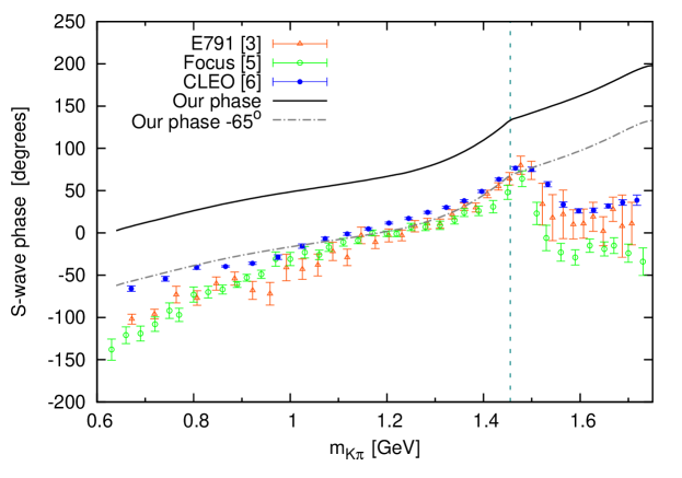
Figure 1: (colour online). $S$-wave phases from the QMI analyses of Refs. Aitala:2005yh ; Bonvicini:2008jw ; Focus2009 . The solid line is the phase of our $S$-wave amplitude with $\alpha=0^{\circ}$ in Eq. (37), whereas the dot-dashed line is the $S$-wave phase with $\alpha=-65^{\circ}$. The dashed line delimits the $K\eta^{\prime}$ threshold.

In order to compare the absolute value of our $S$ wave amplitude with experimental data, we need fix the only two free parameters that occur in our model, namely the normalisation constants $\chi_{S}^{\rm eff}$ and $\chi_{V}^{\rm eff}$. Estimates for the normalisations were given in Eqs. (26) and (34) but in order to perform a careful comparison with experimental results we choose to refine these values. With that aim, we employ the following strategy. The constant $\chi_{V}^{\rm eff}$ is fixed in order to reproduce the value of the sum of all vector submodes in the second column of Table 1. Then, we fix the scalar normalisation $\chi_{S}^{\rm eff}$ requiring the total branching ratio from our model to match the world average of Table 1. Taking the central values for $a_{1}$ and $a_{2}$ given in Eq. (4) this procedure gives

$$\chi_{S}^{\rm eff}=4.9\pm 0.4\,\,\,\mbox{GeV}^{-1}\ ,\qquad\chi_{V}^{\rm eff}=4.4\pm 0.6\,\,\,\mbox{GeV}^{-1}\ ,$$ (38)

in good agreement with our estimates in Eqs. (26) and (34). The uncertainties take into account the error in $a_{1}$ and $a_{2}$ which dominate by far as compared to the relatively small errors of the world averages of Table 1. We are now in a position to compute the scalar branching ratio, shown in Table 1, as well as the fit fractions of the total vector and scalar contributions which are shown in Tables 2 and 3. The model reproduces the dominant $S$-wave contribution and gives fit fractions in fair agreement with the experimental results.

We can now compare the absolute value of our $S$-wave amplitude with experimental results from the QMI analyses. However, since in isobar-like analyses the fit is sensitive only to the relative weights of the amplitudes, in order to compare the measurements with our result we need perform a normalisation. We define a normalised $S$-wave amplitude by

$$\mathcal{A}_{S}^{\mbox{\tiny Norm}}(m_{K\pi_{1}}^{2},m_{K\pi_{2}}^{2})=\frac{\mathcal{A}_{S}}{\left(\int_{\mathcal{D}}\,dm_{K\pi_{1}}^{2}dm_{K\pi_{2}}^{2}\,|\mathcal{A}_{S}|^{2}\right)^{1/2}}\ .$$ (39)

This amplitude, by construction, is free of any global constants that appear in $\mathcal{A}_{S}$ and has dimension of [Energy]^-2. Interpolating the results from the tables found in Refs. Aitala:2005yh ; Bonvicini:2008jw ; Focus2009 we can calculate the normalised $S$ wave for each experiment. We repeated the same procedure for our total $S$-wave amplitude. The QMI results for the $S$ wave are compared with our model in Fig. 2. Up to $1.55$ GeV the agreement of our results with the experimental ones is remarkable.

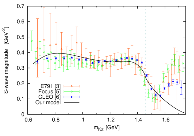
Figure 2: (colour online). Absolute value of the $S$ wave measured in Refs. Aitala:2005yh ; Bonvicini:2008jw ; Focus2009 compared with our model. The amplitudes are normalised according to Eq. (39). The dashed line delimits the $K\eta^{\prime}$ threshold.

Finally, we can perform a Monte Carlo (MC) simulation to obtain a Dalitz plot from our model and compare the diagram and its projections with experimental results. For the lack of a true data set, we resort to a MC simulation of the original E791 data Aitala:2002kr . Reproducing their fit function, we generated a symmetrised Dalitz plot with 14185 independent signal events which corresponds to $6\%$ of background contamination in the total sample Aitala:2002kr . The obtained diagram is shown in Fig. 3a. Then we performed the same exercise for our model and the result is shown in Fig. 3b. It is important to remark that the shape of the Dalitz plot is related to the global phase shift of Eq. (37). In the words of Ref. Aitala:2005yh , the asymmetry in the $K\pi$ $P$-wave bands reflects the value of $\alpha$. We have checked that taking $\alpha=0^{\circ}$ in Eq. (37) reverses the observed asymmetry, i.e., the high-energy part of the Dalitz is more populated than the low-energy corner. Consequently, we confirm the finding of Ref. Aitala:2005yh : the asymmetry pattern in the Dalitz plot is a direct consequence of the global phase difference between the $S$- and $P$-wave phases. Finally, in Fig. 4 we show the projections of the diagrams of Figs. 3a and 3b. The results for our model with $\alpha=-65^{\circ}$ and the simulated E791 data agree quite well. The discrepancy in Fig. 4a around 1 GeV² is due to the interference pattern between the $S$ and $P$ waves. This could be fixed through a fit to real data, which would give a refined value for $\alpha$. One also sees around 2.5 GeV² a second discrepancy, seen in both Figs. 4a and 4c, that is a consequence of the disagreement of our $S$ wave with respect to the experimental ones for $m_{K\pi}>1.45$ GeV, as shown in Fig. 2. Small isospin-breaking effects in the $P$-wave are to be expected as well, since the vector $K\pi$ form factor employed here was obtained from $\tau^{-}\to K\pi\,\nu_{\tau}$ decay data Boito:2008fq where the charged vector resonances intervene.

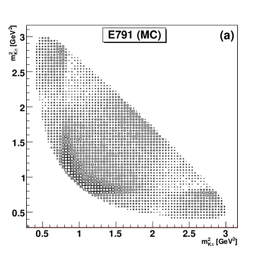
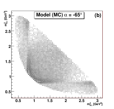
Figure 3: (a) Monte Carlo simulation for the Dalitz plot of the E791 original analysis Aitala:2002kr (b) Same for our model with a global shift of $-65^{\circ}$ degrees in the $S$-wave phase (see text and Fig. 1). The number of independent events is 14185, which correspond to the estimate of the signal events in Ref. Aitala:2002kr .

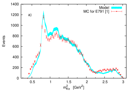
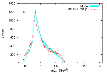
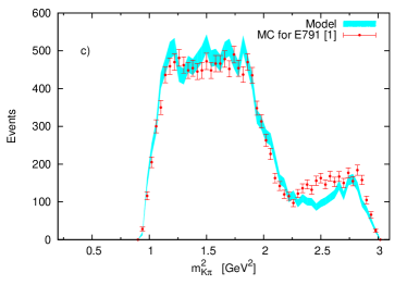
Figure 4: (colour online). Projections from the MC generated Dalitz plots of Figs. 3a and 3b. The error bars and the bands represent solely statistical fluctuations. (a) Total projection, (b) high-energy projection, (c) low-energy projection.

As a final comment, we remark that we do not include $(\pi^{+}\pi^{+})_{I=2}$ interactions in our model. Within the framework employed here this contribution does not appear. Since the inclusion of an ad-hoc $I=2$ amplitude would downgrade the model, we prefer to consider only the $I=1/2$ FSIs. Additionally, $(\pi^{+}\pi^{+})_{I=2}$ scattering is entirely non-resonant Amsler:2008zzb with a slow variation of the corresponding phase shift I2 , indicating that interactions in this channel are weak. Furthermore, from an experimental point of view, the need for the $I=2$ amplitude is not well established and requires further confirmation (see Table 2).

IV Summary and discussion

We have presented a model aimed at describing the decay $D^{+}\to K^{-}\pi^{+}\pi^{+}$. The weak amplitude is described within the effective Hamiltonian framework with the hypothesis of factorisation. The $K\pi$ hadronic FSIs are treated in a quasi two-body approach by means of the well defined scalar and vector $K\pi$ form factors, thereby imposing analyticity, unitarity and chiral symmetry constraints. We used the experimental values for the total and $P$-wave branching ratios to fix the two free parameters in the model. The relative global phase difference between the $S$ and $P$ waves was fixed phenomenologically using the experimental results of Ref. Bonvicini:2008jw .

The use of the $K\pi$ scalar form factor is shown to provide a good description of the $S$-wave FSIs. Both the modulus and the phase of our $S$ wave compare well with experimental data up to $m_{K\pi}\lesssim 1.5$ GeV. It is worth mentioning that the form factor we used has a pole that can be identified with the $\kappa$. Furthermore, the model is able to reproduce the experimental fit fractions and the total $S$-wave branching ratio. Finally, the Dalitz plot arising from the model agrees with a MC simulated data set.

The main hypotheses of our model are the factorisation of the weak decay amplitude and the quasi two-body nature of the FSIs. Therefore, the success of our description for $m_{K\pi}\lesssim 1.5$ GeV suggests that, in this domain, the physics of the decay is dominated by two-body $K\pi$ interactions. We are led to conclude that effects not included in our model such as the $I=3/2$ non-resonant $K\pi$ $S$ wave, the non-resonant $I=2$ $\pi^{+}\pi^{+}$ interactions and genuine three-body interactions, could be considered as corrections to the general picture described here.

Part of the discrepancy observed in our Dalitz plot is due to the disaccord of our $S$-wave amplitude for $m_{K\pi}\gtrsim 1.5$ GeV. A possible cause for this disagreement is the fact that factorisation in a three-body decay is expected to break down close to the edges of the Dalitz plot BenoitBKpipi ; Beneke . Furthermore, in this region, the kinematical configuration of the final state momenta renders the quasi two-body treatment less trustworthy as well. Finally, our model does not include the tensor component. Although marginal, this amplitude has a non-trivial distribution in the phase space and could induce sizable interference effects in our plots. In the vector channel, we find puzzling that the $K^{*}(1410)$, which gives a sizable contribution for $\tau^{-}\to K\pi\nu_{\tau}$ JPP2 ; Boito:2008fq , is hardly seen in experimental analyses of $D^{+}\to K^{-}\pi^{+}\pi^{+}$.

In conclusion, since we do not fit the Dalitz plot we think that the agreement between the model and the experimental data is satisfactory.

Appendix A $K\pi$ form factors

The scalar and vector $K\pi$ form factors employed in this work were obtained respectively in Ref. Jamin:2006tj and Ref. Boito:2008fq . The details can be found in the original references but for the sake of completeness we briefly summarise here how they are obtained.

A.1 Scalar $K\pi$ form factor

The framework for the determination of the scalar $K\pi$ form factor, $F_{0}^{K\pi}(s)$, is described in detail in Ref. Jamin:2001zq . The results were numerically updated later and we employed in our numerical analysis the latest version given in Ref. Jamin:2006tj . In Ref. Jamin:2001zq , the authors solved a generalised Omnès problem where three channels, namely $K\pi$, $K\eta$ and $K\eta^{\prime}$, are taken into account. In this framework, the scalar form factor for channel $k$, $F_{0}^{k}(s)$ (where $1\equiv K\pi$, $2\equiv K\eta$ and $3\equiv K\eta^{\prime}$), can be cast as a sum over the three channels as

$$F_{0}^{k}(s)=\frac{1}{\pi}\sum_{j=1}^{3}\,\int\limits_{s_{j}}^{\infty}ds^{\prime}\,\frac{\sigma_{j}(s^{\prime})F_{0}^{j}(s^{\prime})t_{0}^{{k\to j}}(s^{\prime})^{*}}{(s^{\prime}-s-i\epsilon)}\ .$$ (40)

In the last equation, $s_{j}$ is the threshold for channel $j$, $\sigma_{j}(s)$ are two-body phase-space factors and $t_{0}^{k\to j}$ are partial wave $T$-matrix elements for the scattering $k\to j$. The form factors are obtained solving the coupled dispersion relations arising from Eq. (40). This is done imposing chiral symmetry constraints and using $T$-matrix elements from Ref. JOPscatt that provide a good description of scattering data. One recovers the elastic approximation by considering solely the contribution of the channel $k$ to the right-hand side of Eq. (40), which is then reduced to the usual Omnès equation Omnes:1958hv .

A.2 Vector $K\pi$ form factor

The vector $K\pi$ form factor, $F_{+}^{K\pi}(s)$, employed in this work was obtained in Ref. Boito:2008fq within a dispersive representation from fits to $\tau^{-}\to K\pi\nu_{\tau}$ data obtained by the Belle collaboration Belle . The reduced vector form factor $\tilde{F}_{+}^{K\pi}(s)\equiv F_{+}^{K\pi}(s)/F_{+}^{K\pi}(0)$ is written in terms of a three-times-subtracted dispersion relation that takes the form

$$\tilde{F}_{+}^{K\pi}(s)=\exp\left[\alpha_{1}\frac{s}{m_{\pi}^{2}}+\frac{1}{2}\alpha_{2}\frac{s^{2}}{m_{\pi}^{4}}+\frac{s^{3}}{\pi}\int\limits_{s_{K\pi}}^{s_{\rm cut}}ds^{\prime}\frac{\delta_{1}^{K\pi}(s^{\prime})}{(s^{\prime})^{3}(s^{\prime}-s-i0)}\right]\ ,$$ (41)

where $s_{K\pi}$ is the $K\pi$ threshold and $\delta_{1}^{K\pi}$ is the form-factor phase. The subtraction constants $\alpha_{1}$ and $\alpha_{2}$ can easily be related to the slope parameters $\lambda_{+}^{(n)}$, which appear in the Taylor expansion of $\tilde{F}_{+}^{K\pi}(s)$ around $s=0$,

$$\tilde{F}_{+}^{K\pi}(s)=1+\lambda^{\prime}_{+}\frac{s}{m_{\pi}^{2}}+\frac{1}{2}\lambda^{\prime\prime}_{+}\frac{s^{2}}{m_{\pi}^{4}}+\cdots\ ,$$ (42)

as $\lambda^{\prime}_{+}=\alpha_{1}$ and $\lambda^{\prime\prime}_{+}=\alpha_{2}+\alpha_{1}^{2}$. The cutoff $s_{\rm cut}$ is introduced as the upper limit of the Omnès integral to study the importance of the high-energy region which is strongly suppressed by the factor $s^{\prime 3}$ in the denominator of the integrand of Eq. (41). Furthermore, within the elastic region, $\delta_{1}^{K\pi}$ is the $P$-wave $I=1/2$ $K\pi$ scattering phase shift. An advantage of the three-times-subtracted form of $\tilde{F}_{+}^{K\pi}(s)$ is to make the results less sensitive to deficiencies of the phase shift in the higher-energy region. Then, the integral in Eq. (41) emphasises the lower-energy domain (elastic domain), for which one can provide a reliable model for the phase shift. The description of $\delta_{1}^{K\pi}$ we used is inspired by RChT and includes the contribution of two vector resonances namely the $K^{*}(892)$ and the $K^{*}(1410)$. The detailed expressions can be found in Ref. Boito:2008fq .

References

- (1) E. M. Aitala et al. [E791 Collaboration], Phys. Rev. Lett. 89 121801 (2002) [arXiv:hep-ex/0204018].
- (2) E. M. Aitala et al. [E791 Collaboration], Phys. Rev. Lett. 86, 770 (2001) [arXiv:hep-ex/0007028].
- (3) E. M. Aitala et al. [E791 Collaboration], Phys. Rev. D 73, 032004 (2006) [Erratum-ibid. D 74, 059901 (2006)] [arXiv:hep-ex/0507099].
- (4) J. M. Link et al. [FOCUS Collaboration] and M. Pennington, Phys. Lett. B 653, 1 (2007) [arXiv:0705.2248 [hep-ex]].
- (5) J. M. Link et al. [FOCUS Collaboration], arXiv:0905.4846 [hep-ex].
- (6) G. Bonvicini et al. [CLEO Collaboration], Phys. Rev. D 78, 052001 (2008) [arXiv:0802.4214 [hep-ex]].
- (7) E. van Beveren, T. A. Rijken, K. Metzger, C. Dullemond, G. Rupp and J. E. Ribeiro, Z. Phys. C 30, 615 (1986) [arXiv:0710.4067 [hep-ph]].
- (8) D. Black, A. H. Fariborz, F. Sannino and J. Schechter, Phys. Rev. D 58, 054012 (1998) [arXiv:hep-ph/9804273].
- (9) J. A. Oller and E. Oset, Phys. Rev. D 60, 074023 (1999) [arXiv:hep-ph/9809337].
- (10) M. Jamin, J. A. Oller and A. Pich, Nucl. Phys. B 587, 331 (2000) [arXiv:hep-ph/0006045].
- (11) S. Descotes-Genon and B. Moussallam, Eur. Phys. J. C 48, 553 (2006) [arXiv:hep-ph/0607133].
- (12) I. Caprini, G. Colangelo and H. Leutwyler, Phys. Rev. Lett. 96, 132001 (2006) [arXiv:hep-ph/0512364].
- (13) S. M. Roy, Phys. Lett. B 36, 353 (1971).
- (14) J. Gasser and H. Leutwyler, Nucl. Phys. B 250, 465 (1985).
- (15) M. Artuso, B. Meadows and A. A. Petrov, Ann. Rev. Nucl. Part. Sci. 58, 249 (2008) [arXiv:0802.2934 [hep-ph]].
- (16) J. A. Oller, Phys. Rev. D 71, 054030 (2005) [arXiv:hep-ph/0411105].
- (17) J. A. Oller, E. Oset and J. R. Pelaez Phys. Rev. Lett. 80, 3452 (1998) [arXiv:hep-ph/9803242].
- (18) M. Wirbel, B. Stech and M. Bauer, Z. Phys. C 29, 637 (1985).
- (19) M. Bauer, B. Stech and M. Wirbel, Z. Phys. C 34, 103 (1987).
- (20) M. Diakonou and F. Diakonos, Phys. Lett. B216 436 (1989).
- (21) C. Amsler et al. [Particle Data Group], Phys. Lett. B 667, 1 (2008).
- (22) S. Gardner and U.-G. Meißner, Phys. Rev. D 65, 094004 (2002) [arXiv:hep-ph/0112281].
- (23) S. Gardner and J. Tandean, Phys. Rev. D 69, 034011 (2004) [arXiv:hep-ph/0308228].
- (24) U.-G. Meißner and J. A. Oller, Nucl. Phys. A 679, 671 (2001) [arXiv:hep-ph/0005253].
- (25) A. Furman, R. Kamiński, L. Leśniak and B. Loiseau, Phys. Lett. B 622, 207 (2005) [arXiv:hep-ph/0504116].
- (26) B. El-Bennich, A. Furman, R. Kamiński, L. Leśniak and B. Loiseau, Phys. Rev. D 74, 114009 (2006) [arXiv:hep-ph/0608205].
- (27) D. R. Boito, J.-P. Dedonder, B. El-Bennich, O. Leitner, and B. Loiseau, Phys. Rev. D 79, 034020 (2009) [arXiv:0812.3843 [hep-ph]].
- (28) B. El-Bennich, A. Furman, R. Kamiński, L. Leśniak, B. Loiseau, and B. Moussallam, Phys. Rev. D 79, 094005 (2009) [arXiv:0902.3645 [hep-ph]].
- (29) I. Bediaga, C. Göbel and R. Méndez-Galain, Phys. Rev. Lett. 78, 22 (1997) [arXiv:hep-ph/9605442].
- (30) I. Bediaga, C. Göbel and R. Méndez-Galain, Phys. Rev. D 56, 4268 (1997) [arXiv:hep-ph/9704437].
- (31) C. Dib and R. Rosenfeld, Phys. Rev. D 63, 117501 (2001) [arXiv:hep-ph/0006145].
- (32) H. Y. Cheng, Phys. Rev. D 67, 034024 (2003) [arXiv:hep-ph/0212117].
- (33) B. El-Bennich, O. Leitner, J.-P. Dedonder, and B. Loiseau, Phys. Rev. D 79, 076004 (2009) [arXiv:0810.5771 [hep-ph]].
- (34) A. J. Buras, Nucl. Phys. B 434, 606 (1995) [arXiv:hep-ph/9409309].
- (35) A. J. Buras, M. Jamin, M. E. Lautenbacher and P. H. Weisz, Nucl. Phys. B 370, 69 (1992) [Addendum-ibid. B 375, 501 (1992)]; M. Ciuchini, E. Franco, G. Martinelli and L. Reina, Nucl. Phys. B 415, 403 (1994) [arXiv:hep-ph/9304257].
- (36) M. Jamin, J. A. Oller and A. Pich, Nucl. Phys. B 622, 279 (2002) [arXiv:hep-ph/0110193].
- (37) M. Jamin, J. A. Oller and A. Pich, Eur. Phys. J. C 24, 237 (2002) [arXiv:hep-ph/0110194].
- (38) M. Jamin, J. A. Oller and A. Pich, JHEP 0402, 047 (2004) [arXiv:hep-ph/0401080].
- (39) M. Jamin, J. A. Oller and A. Pich, Phys. Rev. D 74, 074009 (2006) [arXiv:hep-ph/0605095].
- (40) M. Jamin, A. Pich and J. Portolés, Phys. Lett. B 640, 176 (2006) [arXiv:hep-ph/0605096].
- (41) M. Jamin, A. Pich and J. Portolés, Phys. Lett. B 664, 78 (2008) [arXiv:0803.1786 [hep-ph]].
- (42) B. Moussallam, Eur. Phys. J. C 53, 401 (2008) [arXiv:0710.0548 [hep-ph]].
- (43) D. R. Boito, R. Escribano and M. Jamin, Eur. Phys. J. C 59, 821 (2009) [arXiv:0807.4883 [hep-ph]]; D. R. Boito, R. Escribano and M. Jamin, PoS EFT09, 064 (2009) [arXiv:0904.0425 [hep-ph]].
- (44) G. Ecker, J. Gasser, A. Pich, and E. de Rafael, Nucl. Phys. B 321, 311 (1989).
- (45) D. Epifanov et al. [Belle Collaboration], Phys. Lett. B 654, 65 (2007) [arXiv:0706.2231 [hep-ex]].
- (46) L. Wolfenstein, Phys. Rev. Lett. 51, 1945 (1983).
- (47) L. Widhalm et al. [Belle Collaboration], Phys. Rev. Lett. 97, 061804 (2006) [arXiv:hep-ex/0604049].
- (48) R. Omnès, Nuovo Cim. 8, 316 (1958).
- (49) J. H. Kühn and E. Mirkes, Z. Phys. C 56, 661 (1992) [Erratum-ibid. C 67, 364 (1995)].
- (50) B. Bajc, S. Fajfer, R. J. Oakes and T. N. Pham, Phys. Rev. D 58, 054009 (1998) [arXiv:hep-ph/9710422].
- (51) D. Melikhov and B. Stech, Phys. Rev. D 62, 014006 (2000) [arXiv:hep-ph/0001113].
- (52) A. Abada, D. Becirevic, P. Boucaud, J. M. Flynn, J. P. Leroy, V. Lubicz and F. Mescia [SPQcdR collaboration], Nucl. Phys. Proc. Suppl. 119, 625 (2003) [arXiv:hep-lat/0209116].
- (53) S. Fajfer and J. F. Kamenik, Phys. Rev. D 72, 034029 (2005) [arXiv:hep-ph/0506051].
- (54) K. M. Watson, Phys. Rev. 88, 1163 (1952).
- (55) N. N. Achasov and G. N. Shestakov, Phys. Rev. D 67, 114018 (2003) [arXiv:hep-ph/0302220].
- (56) M. Beneke, talk presented at “Three-Body Charmless Decays Workshop”, February 1-3, 2006, LPNHE, Paris; http://lpnhe-babar.in2p3.fr/3BodyCharmlessWS/.