Modal approximations to damped linear systems

Abstract

We consider a finite dimensional damped second order system and obtain spectral inclusion theorems for the related quadratic eigenvalue problem. The inclusion sets are the ’quasi Cassini ovals’ which may greatly outperform standard Gershgorin circles. As the unperturbed system we take a modally damped part of the system; this includes the known proportionally damped models, but may give much sharper estimates. These inclusions are then applied to derive some easily calculable sufficient conditions for the overdampedness of a given damped system.

1 Introduction and preliminaries

A damped linear system without gyroscopic forces is governed by the differential equation

$$M\ddot{x}+C\dot{x}+Kx=f(t).$$ (1)

Here $x=x(t)$ is an $\mathbb{R}^{n}$-valued function of time $t\in\mathbb{R}$; $M,C,K$ are real symmetric matrices of order $n$. Typically $M,K$ are positive definite whereas $C$ is positive semidefinite. The physical meaning of these objects is

$$x(t)$$ position or displacement

$$M$$ mass

$$C$$ damping

$$K$$ stiffness

$$f(t)$$ external force

If in the homogeneous equation above we insert $x(t)=e^{\lambda t}x$, $x$ constant, we obtain

$$(\lambda^{2}M+\lambda C+K)x=0$$ (2)

which is called the quadratic eigenvalue problem, attached to (1), $\lambda$ is an eigenvalue and $x$ a corresponding eigenvector.

The quadratic eigenvalue problem may have poor spectral theory in spite of the hermiticity and positive (semi)definiteness of $M.C,K$. There always exists a non-singular matrix $\Phi$ such that

$$\Phi^{T}M\Phi=I,\quad\Phi^{T}K\Phi=\Omega=\operatorname{diag}(\omega_{1}^{2},\ldots,\omega_{n}^{2}).$$ (3)

If the matrix $\Phi$ can be chosen such that also

$$D=\Phi^{T}C\Phi$$ (4)

is diagonal then the system is called modally damped.

While (3) is the standard spectral decomposition of a symmetric positive definite matrix pair. a simultaneous achieving of (4) is rather an exception being equivalent to the generalised commutativity property

$$CK^{-1}M=MK^{-1}C.$$ (5)

However, as an approximation, modal damping is attractive since it is handled by the standard theory and numerics of Hermitian matrices. The aim of this paper is to assess modal approximations of general damped systems. More precisely, we will derive spectral inclusion theorems for eigenvalues where the unperturbed system is modally damped. There is some hierarchy among various modal approximations of a given damped system and we will investigate this issue as well. Our inclusion sets will not be circles, we will call them quasi Cassini ovals. We will show that our ovals outdo classical Gershgorin circles. A special case are overdamped systems the eigenvalues of which are particularly well behaved, there ovals reduce to intervals and inclusions of Wielandt-Hoffman type will be derived. Finally, we will derive new calculable sufficient conditions for the overdampedness of a given system.

2 Modal approximation

Some, rather rough, facts on the positioning of the eigenvalues are given in [4]. Further, more detailed, information is obtained by the perturbation theory. A simplest thoroughly known system is the undamped one. Next to this lie the modally damped systems.

A simplest eigenvalue inclusion for a general matrix $A$ close to a matrix $A_{0}$ is

$$\sigma(A)\subseteq{\cal G}_{1}=\{\lambda:\ \|(A-A_{0})(A_{0}-\lambda I)^{-1}\|<1\}$$ (6)

Obviously ${\cal G}_{1}\subseteq{\cal G}_{2}$ with

$${\cal G}_{2}=\{\lambda:\ \|(A_{0}-\lambda I)^{-1}\|^{-1}\leq\|(A-A_{0})\|\}.$$ (7)

This is valid for any matrices $A,A_{0}$. Using $\Phi$, $\Omega$ from (3) we set

$$y_{1}=\Omega\Phi^{-T}x,\quad y_{2}=\lambda\Phi^{-T}x,$$

so the quadratic eigenvalue equation (2) is equivalent to

$$Ay=\lambda y.$$ (8)

Here we have set

$$A=\left[\begin{array}[]{rr}0&\Omega\\ -\Omega&-D\\ \end{array}\right],\quad A_{0}=\left[\begin{array}[]{rr}0&\Omega\\ -\Omega&0\\ \end{array}\right].$$ (9)

Hence

$$A-A_{0}=\left[\begin{array}[]{rr}0&0\\ 0&-D\\ \end{array}\right].$$

The matrix $A_{0}$ is skew-symmetric and therefore normal, so $\|(A_{0}-\lambda I)^{-1}\|^{-1}=\mathrm{dist}(\lambda,\sigma(A_{0}))$ hence

$${\cal G}_{2}=\{\lambda:\ \mathrm{dist}(\lambda,\sigma(A_{0})\leq\|(A-A_{0})\|\}$$ (10)

where

$$\|(A-A_{0})\|=\|D\|=\|L_{2}^{-1}CL_{2}^{-T}\|=\max\frac{x^{T}Cx}{x^{T}Mx}$$ (11)

is the largest eigenvalue of the matrix pair $C,M$. We may say that here ’the size of the damping is measured relative to the mass’.

Thus, the perturbed eigenvalues are contained in the union of the disks of radius $\|D\|$ around $\sigma(A_{0})$.

Remark 2.1.

In fact, $\sigma(A)$ is also contained in the union of the disks

$$\{\lambda:\ |\lambda\mp i\omega_{j}|\leq R_{j}\}$$ (12)

with

$$R_{j}=\sum_{k=1}^{n}|d_{kj}|.$$ (13)

(Replace the spectral norm in (6) by the norm $\|\cdot\|_{1}$).

The bounds obtained above are, in fact, too crude, since we have not taken into account the structure of the perturbation $A-A_{0}$ which has a remarkable zero pattern.

Instead of working with the matrix $A$ we may turn back to the original quadratic eigenvalue problem in the representation in the form (see (3) and (9))

$$\det(\lambda^{2}I+\lambda D+\Omega^{2})=0.$$

The inverse

$$(\lambda^{2}I+\lambda D+\Omega^{2})^{-1}=$$

$$(\lambda^{2}I+\Omega^{2})^{-1}(I+\lambda D(\lambda^{2}I+\Omega^{2})^{-1})^{-1}$$

exists, if

$$\|D(\lambda^{2}I+\Omega^{2})^{-1}\||\lambda|<1$$ (14)

which is implied by

$$\|(\lambda^{2}I+\Omega^{2})^{-1}\|\|D\||\lambda|=\frac{\|D\||\lambda|}{\min_{j}(|\lambda-i\omega_{j}||\lambda+i\omega_{j}|)}<1$$ (15)

Thus,

$$\sigma(A)\subseteq\cup_{j}{\cal C}(i\omega_{j},-i\omega_{j},\|D\|),$$ (16)

where the set

$${\cal C}(\lambda_{+},\lambda_{-},r)=\{\lambda:|\lambda-\lambda_{+}||\lambda-\lambda_{-}|\leq|\lambda|r\}$$ (17)

will be called quasi Cassini ovals with foci $\lambda_{\pm}$ and extension $r$. This is in analogy with the standard Cassini ovals where on the right hand side instead of $|\lambda|r$ one has just $r^{2}$. (The latter also appear in eigenvalue bounds in somewhat different context.) We note the obvious relation

$${\cal C}(\lambda_{+},\lambda_{-},r)\subset{\cal C}(\lambda_{+},\lambda_{-},r^{\prime}),\quad\mbox{whenever }r<r^{\prime}.$$ (18)

The quasi Cassini ovals are qualitatively similar to the standard ones; they can consist of one or two components; the latter case occurs when $r$ is sufficiently small with respect to $|\lambda_{+}-\lambda_{-}|$. In this case the ovals in (16) are approximated by the disks

$$|\lambda\pm i\omega_{j}|\leq\frac{\|D\|}{2}$$ (19)

and this is one half of the bound in (10), (11).

Remark 2.2.

$\sigma(A)$ is also contained in the union of the ovals

$${\cal C}(i\omega_{j},-i\omega_{j},\|\Omega^{-1}D\Omega^{-1}\|\omega_{j}^{2}).$$ (20)

Indeed, instead of inverting $\lambda^{2}I+\lambda D+\Omega^{2}$ invert $\lambda^{2}\Omega^{-2}+\lambda\Omega^{-1}D\Omega^{-1}+I$.

Remark 2.3.

$\sigma(A)$ is also contained in the union of the ovals

$${\cal C}(i\omega_{j},-i\omega_{j},R_{j})$$ (21)

and also

$${\cal C}(i\omega_{j},-i\omega_{j},\rho_{j}\omega_{j}^{2})$$ (22)

with

$$\rho_{j}=\sum_{{k=1\atop k\neq j}}^{n}\frac{|d_{kj}|}{\omega_{k}\omega_{j}}.$$ (23)

The just considered undamped approximation was just a prelude to the main topic of this section, namely the modal approximation. The modally damped systems are so much simpler than the general ones that practitioners often substitute the true damping matrix by some kind of ’modal approximation’. Most typical such approximations in use are of the form

$$C_{prop}=\alpha M+\beta K$$ (24)

where $\alpha,\beta$ are chosen in such a way that $C_{prop}$ be in some sense as close as possible to $C$, for instance,

$$\mathrm{Tr}\left[(C-\alpha M-\beta K)W(C-\alpha M-\beta K)\right]=\min,$$ (25)

where $W$ is some convenient positive definite weight matrix. This is a proportional approximation. In general such approximations may go quite astray and yield thoroughly false predictions. We will now assess them in a more systematic way.

A modal approximation to the system (1) is obtained by first representing it in modal coordinates by the matrices $D$, $\Omega$ and then by replacing $D$ by its diagonal part

$$D^{0}=\operatorname{diag}(d_{11},\ldots,d_{nn}).$$ (26)

The off-diagonal part $D^{\prime}=D-D^{0}$ is considered a perturbation. Again we can work in the phase space or with the original quadratic eigenvalue formulation. In the first case we can make perfect shuffling to obtain

$$A=(A_{i,j}),\quad A_{ii}=\left[\begin{array}[]{rr}0&\omega_{i}\\ -\omega_{i}&d_{ii}\\ \end{array}\right],\quad A_{ij}=\left[\begin{array}[]{rr}0&0\\ 0&d_{ij}\\ \end{array}\right]$$ (27)

$$A_{0}=\operatorname{diag}(A_{11},\ldots,A_{nn}).$$ (28)

So, for $n=3$

$$A=\left[\begin{array}[]{cc|cc|cc}0&\omega_{1}&0&0&0&0\\ -\omega_{1}&-d_{11}&0&-d_{12}&0&-d_{13}\\ \hline\cr 0&0&0&\omega_{2}&0&0\\ 0&-d_{12}&-\omega_{2}&-d_{22}&0&-d_{23}\\ \hline\cr 0&0&0&0&0&\omega_{3}\\ 0&-d_{13}&0&-d_{23}&-\omega_{3}&-d_{33}\\ \end{array}\right].$$

Then

$$\|(A_{0}-\lambda I)^{-1}\|^{-1}=\max_{j}\|(A_{jj}-\lambda I)^{-1}\|^{-1}.$$

Even for $2\times 2$-blocks any common norm of $(A_{jj}-\lambda I)^{-1}$ seems complicated to express in terms of disks or other simple regions, unless we diagonalise each $A_{jj}$ as

$$S_{j}^{-1}A_{jj}S_{j}=\left[\begin{array}[]{rr}\lambda_{+}^{j}&0\\ 0&\lambda_{-}^{j}\\ \end{array}\right],\quad\lambda_{\pm}^{j}=\frac{-d_{jj}\pm\sqrt{d_{jj}^{2}-4\omega_{j}^{2}}}{2}.$$ (29)

As is directly verified,

$$\kappa(S_{j})=\sqrt{\frac{1+\theta_{j}^{2}}{|1-\theta_{j}^{2}|}},\quad\theta_{j}=\frac{d_{jj}}{2\omega_{j}}.$$

with

$$\theta_{j}=\frac{d_{jj}}{2\omega_{j}}.$$

Set $S=\operatorname{diag}(S_{11},\ldots,S_{nn})$ and

$$A^{\prime}=S^{-1}AS=A_{0}^{\prime}+A^{\prime\prime}$$

then

$$A_{0}^{\prime}=\operatorname{diag}(\lambda_{\pm}^{1},\ldots,\lambda_{\pm}^{n}),$$

$$A_{jk}^{\prime\prime}=S_{j}^{-1}A_{jk}^{\prime}S_{k},\quad A^{\prime\prime}=S^{-1}A^{\prime}S$$

Now the general perturbation bound (10), applied to $A_{0}^{\prime},A^{\prime\prime}$, gives

$$\sigma(A)\subseteq\cup_{j,\pm}\{\lambda:\ |\lambda-\lambda_{\pm}^{j}|\leq\kappa(S)\|D^{\prime}\|\}.$$ (30)

There is a related ’Gershgorin-type bound’

$$\sigma(A)\subseteq\cup_{j,\pm}\{\lambda:\ |\lambda-\lambda_{\pm}^{j}|\leq\kappa(S_{j})r_{j}\}$$ (31)

with

$$r_{j}=\sum_{k=1\atop j\neq i}^{n}\|d_{jk}\|.$$ (32)

To show this we replace the spectral norm $\|\cdot\|$ in (6) by the norm $\||\cdot\||_{1}$, defined as

$$\||A\||_{1}:=\max_{j}\sum_{k}\|A_{kj}\|$$

where the norms on the right hand side are spectral. Thus, (6) will hold, if

$$\max_{j}\sum_{k}\|(A-A_{0})_{kj}\|\|(A_{jj}-\lambda I)^{-1}\|<1$$

Taking into account the equality

$$\|(A-A_{0})_{kj}\|=\left\{\begin{array}[]{rr}|d_{kj}|,&k\neq j\\ 0&k=j\end{array}\right.$$

$\lambda\in\sigma(A)$ implies

$$r_{j}\geq\|(A_{jj}-\lambda I)^{-1}\|\geq\frac{\min\{|\lambda-\lambda_{+}^{j}|,|\lambda-\lambda_{-}^{j}|\}}{\kappa(S_{j})}$$

and this is (31).

Note that the bounds (30) and (31) are poor whenever the modal approximation is close to a critically damped eigenvalue.

Better bounds are expected, if we work directly with the quadratic eigenvalue equation. The inverse

$$(\lambda^{2}I+\lambda D+\Omega^{2})^{-1}=$$

$$(\lambda^{2}I+\lambda D^{0}+\Omega^{2})^{-1}(I+\lambda D^{\prime}(\lambda^{2}I+\lambda D^{0}+\Omega^{2})^{-1})^{-1}$$

exists, if

$$\|D^{\prime}(\lambda^{2}I+\lambda D^{0}+\Omega^{2})^{-1}\||\lambda|<1$$ (33)

which is insured, if

$$\|(\lambda^{2}I+\lambda D^{0}+\Omega^{2})^{-1}\|\|D^{\prime}\||\lambda|=\frac{\|D^{\prime}\||\lambda|}{\min_{j}(|\lambda-\lambda_{+}^{j}||\lambda-\lambda_{-}^{j}|)}<1$$ (34)

Thus,

$$\sigma(A)\subseteq\cup_{j}{\cal C}(\lambda_{+}^{j},\lambda_{-}^{j},\|D^{\prime}\|).$$ (35)

These ovals will always have both foci either real or complex conjugate. If $r=\|D^{\prime}\|$ is small with respect to $|\lambda_{+}^{j}-\lambda_{-}^{j}|=\sqrt{|d_{jj}^{2}-4\omega_{j}^{2}|}$ then either $|\lambda-\lambda_{+}^{j}|$ or $|\lambda-\lambda_{-}^{j}|$ is small. In the first case the inequality $|\lambda-\lambda_{+}^{j}||\lambda-\lambda_{-}^{j}|\leq|\lambda|r$ is approximated by

$$|\lambda-\lambda_{+}^{j}|\leq\frac{|\lambda_{+}^{j}|r}{|\lambda_{+}^{j}-\lambda_{-}^{j}|}=r\left\{\begin{array}[]{ll}\frac{\omega_{j}}{\sqrt{d_{jj}^{2}-4\omega_{j}^{2}}}&d_{jj}<2\omega_{j}\\ \mbox{}\\ \frac{d_{jj}-\sqrt{d_{jj}^{2}-4\omega_{j}^{2}}}{\sqrt{d_{jj}^{2}-4\omega_{j}^{2}}}&d_{jj}>2\omega_{j}\\ \end{array}\right.$$ (36)

and in the second

$$|\lambda-\lambda_{-}^{j}|\leq\frac{|\lambda_{-}^{j}|r}{|\lambda_{+}^{j}-\lambda_{-}^{j}|}=r\left\{\begin{array}[]{ll}\frac{\omega_{j}}{\sqrt{d_{jj}^{2}-4\omega_{j}^{2}}}&d_{jj}<2\omega_{j}\\ \mbox{}\\ \frac{d_{jj}+\sqrt{d_{jj}^{2}-4\omega_{j}^{2}}}{\sqrt{d_{jj}^{2}-4\omega_{j}^{2}}}&d_{jj}>2\omega_{j}\\ \end{array}\right..$$ (37)

This is again a union of disks. If $d_{jj}\approx 0$ then their radius is $\approx r/2$. If $d_{jj}\approx 2\omega_{j}$ i.e. $\lambda_{-}=\lambda_{+}\approx-d_{jj}/2$ the ovals look like a single circular disk. For large $d_{jj}$ the oval around the absolutely larger eigenvalue is $\approx r$ (the same behaviour as with (31)) whereas the smaller eigenvalue has the diameter $\approx 2r\omega_{j}^{2}/d_{jj}^{2}$ which is drastically better than (31).

In the same way as before the Gershgorin type estimate is obtained

$$\sigma(A)\subseteq\cup_{j}{\cal C}(\lambda_{+}^{j},\lambda_{-}^{j},r_{j}).$$ (38)

We have called $D^{\prime}$ a modal approximation to $D$ because the matrix $D$ is not uniquely determined by the input matrices $M,C,K$. Different choices of the transformation matrix $\Phi$ give rise to different modal approximations $D^{\prime}$ but the differences between them are mostly non-essential. To be more precise, let $\Phi$ and $\tilde{\Phi}$ both satisfy (3). Then

$$M=\Phi^{-T}\Phi^{-1}=\tilde{\Phi}^{-T}\tilde{\Phi}^{-1},$$

$$K=\Phi^{-T}\Omega^{2}\Phi^{-1}=\tilde{\Phi}^{-T}\Omega^{2}\tilde{\Phi}^{-1}$$

implies that $U=\Phi^{-1}\tilde{\Phi}$ is an orthogonal matrix which commutes with

$$\Omega=\operatorname{diag}(\omega_{1}I_{n_{1}},\ldots,\omega_{s}I_{n_{s}}),\quad\omega_{1}<\cdots<\omega_{s}.$$ (39)

Hence

$$U^{0}=\operatorname{diag}(U_{11},\ldots,U_{ss}),$$

where each $U_{jj}$ is an orthogonal matrix of order $n_{j}$ from (26). Now,

$$\tilde{D}=\tilde{\Phi}^{T}C\tilde{\Phi}=U^{T}\Phi^{T}C\Phi U=U^{T}DU,$$ (40)

$$\tilde{D}_{ij}=U_{i}^{T}D_{ij}U_{j}$$ (41)

and hence

$$\tilde{D}^{\prime}=U^{T}D^{\prime}U.$$ (42)

Now, if the undamped frequencies are all simple, then $U$ is diagonal and the estimates (11) or (16)–(17) remain unaffected by this change of coordinates. Otherwise we replace $\operatorname{diag}(d_{11},\ldots,d_{nn})$ by

$$D^{0}=\operatorname{diag}(D_{11},\ldots,D_{ss})$$ (43)

where $D^{0}$ commutes with $\Omega$. In fact, a general definition of a modal approximation is that it

1. is block-diagonal and

2. commutes with $\Omega$.

The modal approximation with the coarsest possible partition — this is the one whose block dimensions equal the multiplicities in $\Omega$ — is called a maximal modal approximation. Accordingly, we say that $C^{0}=\Phi^{-1}D^{0}\Phi^{-T}$ is a modal approximation to $C$ (and also $M,C^{0},K$ to $M,C,K$).

Proposition 2.4.

Each modal approximation to $C$ is of the form

$$C^{0}=\sum_{k=1}^{s}P_{k}^{*}CP_{k}$$ (44)

where $P_{1},\ldots.P_{s}$ is an $M$-orthogonal decomposition of the identity (that is $P_{k}^{*}=MP_{k}M^{-1}$) and $P_{k}$ commute with the matrix

$$\sqrt{M^{-1}K}=M^{-1/2}\sqrt{M^{-1/2}KM^{-1/2}}M^{1/2}$$

Proof. Use the formula

$$D^{0}=\sum_{k=1}^{s}P_{k}^{0}DP_{k}^{0}$$

with

$$P_{k}^{0}=\operatorname{diag}(0\ldots,I_{n_{k}},\ldots,0,\quad D=\Phi^{T}C\Phi,\quad D^{0}=\Phi^{T}C^{0}\Phi$$

and set $P_{k}=\Phi P_{k}^{0}\Phi^{-1}$. Q.E.D.

It is obvious that the maximal approximation is the best among all modal approximations in the sense that

$$\|D-D^{0}\|_{E}\leq\|D-\hat{D}^{0}\|_{E},$$ (45)

where

$$\hat{D}^{0}=\operatorname{diag}(\hat{D}_{11},\ldots,\hat{D}_{zz})$$ (46)

and $D=(\hat{D}_{ij})$ is any block partition of $D$ which is finer than that in (43). We will now prove that the inequality (45) is valid for the spectral norm also. We shall need the following

Proposition 2.5.

Let $H=(H_{ij})$ be any partitioned Hermitian matrix such that the diagonal blocks $H_{ii}$ are square. Set

$$H^{0}=\operatorname{diag}(H_{11},\ldots,H_{ss}),\quad H^{\prime}=H-H^{0}.$$

Then

$$\lambda_{k}(H)-\lambda_{n}(H)\leq\lambda_{k}(H^{\prime})\leq\lambda_{k}(H)-\lambda_{1}(H)$$ (47)

where $\lambda_{k}(\cdot)$ denotes the non-decreasing sequence of the eigenvalues of any Hermitian matrix.

Proof. By the monotonicity property (Wielandt’s theorem) we have

$$\lambda_{k}(H)-\max_{j}\max\sigma(H_{jj})\leq\lambda_{k}(H^{\prime})\leq\lambda_{k}(H)-\min_{j}\min\sigma(H_{jj}).$$

By the interlacing property,

$$\lambda_{1}(H)\leq\sigma(H_{jj})\leq\lambda_{n}(H).$$

Together we obtain (47). Q.E.D.

From (47) some simpler estimates immediately follow:

$$\|H^{\prime}\|\leq\lambda_{n}(H)-\lambda_{1}(H)=:\mathrm{spread}(H)$$ (48)

and, if $H$ is positive (or negative) semidefinite

$$\|H^{\prime}\|\leq\|H\|.$$ (49)

Now (45) for the spectral norm immediately follows from (49). So, a best bound in (35) is obtained, if $D^{0}=D-D^{\prime}$ is a maximal modal approximation.

Proposition 2.6.

Any modal approximation is better than any proportional one.

Proof. With

$$D_{\mbox{{\it\small prop}}}=\alpha I+\beta\Omega$$

we have

$$|(D-D_{\mbox{{\it\small prop}}})_{ij}|\geq|(D-D^{0})_{ij}|=|D^{0}_{ij}|$$

which implies

$$\|D-D_{\mbox{{\it\small prop}}}\|\geq\|D^{\prime}\|.$$

Q.E.D.

If $D^{0}$ is block diagonal and the corresponding $D^{\prime}=D-D^{0}$ is inserted in (35) then the values $d_{jj}$ from (29) should be replaced by the corresponding eigenvalues of the diagonal blocks $D_{jj}$. But in this case we can further transform $\Omega$ and $D$ by a unitary similarity

$$U=\operatorname{diag}(U_{1},\ldots,U_{s})$$

such that each of the blocks $D_{jj}$ becomes diagonal ($\Omega$ stays unchanged). With this stipulation we may retain the formula (35) unaltered. This shows that taking just the diagonal part $D^{0}$ of $D$ covers, in fact, all possible modal approximations, when $\Phi$ varies over all matrices performing (3).

Similar extension can be made with the bound (38) but then no improvements in general can be guaranteed although they are more likely than not.

By the usual continuity argument it is seen that the number of the eigenvalues in each component of $\cup_{i}{\cal C}(\lambda_{+}^{i},\lambda_{-}^{i},r_{i})$ is twice the number of involved diagonals. In particular, if we have the maximal number of $2n$ components, then each of them contains exactly one eigenvalue.

A strengthening in the sense of Brauer is possible as well. We will show that the spectrum is contained in the union of double ovals, defined as

$${\cal D}(\lambda_{+}^{p},\lambda_{-}^{p},\lambda_{+}^{q},\lambda_{-}^{q},r_{p}r_{q})=$$

$$\{\lambda:|\lambda-\lambda_{+}^{p}||\lambda-\lambda_{-}^{p}||\lambda-\lambda_{+}^{q}||\lambda-\lambda_{-}^{q}|\leq r_{p}r_{q}|\lambda|^{2}\},$$ (50)

where the union is taken over all pairs $p\neq q$ and $\lambda_{\pm}^{p}$ are the solutions of $\lambda^{2}+d_{pp}\lambda+\omega_{p}^{2}=0$ and similarly for $\lambda_{\pm}^{q}$. The proof just mimics the standard Brauer’s one. The quadratic eigenvalue problem is written as

$$(\lambda^{2}+\lambda d_{pp}+\omega_{i}^{2})x_{i}=-\lambda\sum_{j=1\atop J\neq i}^{n}d_{ij}x_{j},$$ (51)

$$(\lambda^{2}+\lambda d_{ii}+\omega_{i}^{2})x_{i}=-\lambda\sum_{j=1\atop J\neq i}^{n}d_{ij}x_{j},$$ (52)

where $|x_{p}|\geq|x_{q}|$ are the two absolutely largest components of $x$. If $x_{q}=0$ then $x_{j}=0$ for all $j\neq p$ and trivially $\lambda\in{\cal D}(\lambda_{+}^{p},\lambda_{-}^{p},\lambda_{+}^{q},\lambda_{-}^{q},r_{p}r_{q})$. If $x_{q}\not=0$ then multiplying the equalities (51) and (52) yields

$$|\lambda-\lambda_{+}^{p}||\lambda-\lambda_{-}^{p}||\lambda-\lambda_{+}^{q}||\lambda-\lambda_{-}^{q}||x_{p}||x_{q}|\leq$$

$$|\lambda|^{2}\sum_{j=1\atop j\neq p}^{n}\sum_{k=1\atop k\neq q}^{n}|d_{pj}||d_{qk}||x_{j}||x_{k}|.$$

Because in the double sum above there is no term with $j=k=p$ we always have $|x_{j}||x_{k}|\leq|x_{p}||x_{q}|$, hence the said sum is bounded by

$$|\lambda|^{2}|x_{p}||x_{q}|\sum_{j=1\atop j\neq p}^{n}|d_{pj}|\sum_{k=1\atop k\neq q}^{n}|d_{qk}|.$$

Thus, our inclusion is proved. As it is immediately seen, the union of all double ovals is contained in the union of all quasi Cassini ovals.

The simplicity of the modal approximation suggests to try to extend it to as many systems as possible. A close candidate for such extension is any system with tightly clustered undamped frequencies, that is, $\Omega$ is close to an $\Omega^{0}$ from (39). Starting again with

$$(\lambda^{2}I+\lambda D+\Omega^{2})^{-1}=$$

$$(\lambda^{2}I+\lambda D^{0}+(\Omega^{0})^{2})^{-1}(I+(\lambda D^{\prime}+Z)+(\lambda^{2}I+\lambda D^{0}+(\Omega^{0})^{2})^{-1})^{-1}$$

with $Z=\Omega^{2}-(\Omega^{0})^{2}$ we immediately obtain

$$\sigma(A)\subseteq\cup_{j}\hat{{\cal C}}(\lambda_{+}^{j},\lambda_{-}^{j},\|D^{\prime}\|,\|Z\|).$$ (53)

where the set

$$\hat{{\cal C}}(\lambda_{+},\lambda_{-},r,q)=\{\lambda:|\lambda-\lambda_{+}||\lambda-\lambda_{-}|\leq|\lambda|r+q\}$$ (54)

will be called modified Cassini ovals with foci $\lambda_{\pm}$ and extensions $r,q$.

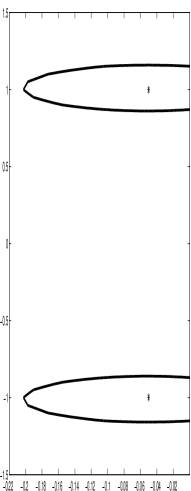
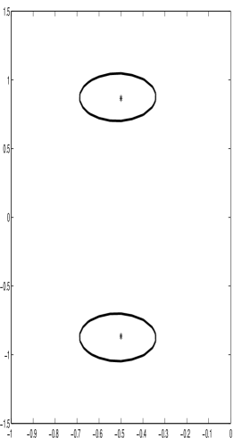
Figure 1: Ovals for $\omega=1;d=0.1,1;\,r=0.3$

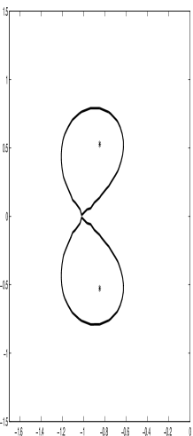
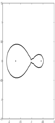
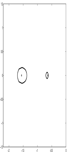
Figure 2: Ovals for $\omega=1;\,d=1.7,2.3,2.2;\,r=0.3,0.3,0.1$

Remark 2.7.

The basis of any modal approximation is the diagonalisation of the matrix pair $M,K$. An analogous procedure with similar results can be performed by diagonalising the pair $M,K$ or $C,K$.

3 Modal approximation and overdampedness

If the systems in the previous section are all overdamped then estimates are greatly simplified as ovals become just intervals. But before going into this a more elementary — and more important — question arises: Can the modal approximation help to decide the overdampedness of a given system?

We begin with some obvious facts the proofs of which are left to the reader.

Proposition 3.1.

If the system $M,C,K$ is overdamped, then the same is true of the projected system

$$M^{\prime}=X^{*}MX,\quad C^{\prime}=X^{*}CX,\quad K^{\prime}=X^{*}KX$$ (55)

where $X$ is any injective matrix. Moreover, the definiteness interval of the former is contained in the one of the latter.

Proposition 3.2.

Let

$$M=\operatorname{diag}(M_{11},\ldots,M_{ss})$$

$$C=\operatorname{diag}(C_{11},\ldots,C_{ss})$$

$$K=\operatorname{diag}(K_{11},\ldots,K_{ss}).$$

Then the system $M,C,K$ is overdamped, if and only if each of $M_{jj},C_{jj},K_{jj}$ is overdamped and their definiteness intervals have a non trivial intersection (which is then the definiteness interval of $M,C,K$)

Corollary 3.3.

If the system $M,C,K$ is overdamped, then the same is true of any of its modal approximations.

Obviously, if a maximal modal approximation is overdamped, then so are all others.

In the following we shall need some well known sufficient conditions for negative definiteness of a general Hermitian matrix $A=(a_{ij})$; these are:

$$a_{jj}<0$$ (56)

for all $j$ and either

$$\|A-\operatorname{diag}(a_{11},\ldots,a_{nn})\|<-\max_{j}a_{jj}$$ (57)

(norm-diagonal dominance) or

$$\sum_{k=1\atop k\neq j}^{n}|a_{kj}|<-a_{jj}\mbox{ for all }j$$ (58)

(Gershgorin-diagonal dominance).

Theorem 3.4.

Let $\Omega$, $D$, $r_{j}$ be from (3), (4), (32), respectively and

$$D^{0}=\operatorname{diag}(d_{11},\ldots,d_{nn}),\quad D^{\prime}=D-D^{0}.$$

Let either

$$\Delta_{j}=(d_{jj}-\|D^{\prime}\|)^{2}-4\omega_{j}^{2}>0\mbox{ for all }j$$ (59)

and

$$p_{-}:=\max_{j}\frac{-d_{jj}+\|D^{\prime}\|-\sqrt{\Delta_{j}}}{2}<\min_{j}\frac{-d_{jj}+\|D^{\prime}\|+\sqrt{\Delta_{j}}}{2}=:p_{+}$$ (60)

or

$$\hat{\Delta}_{j}=(d_{jj}-r_{j})^{2}-4\omega_{j}^{2}>0\mbox{ for all }j$$ (61)

and

$$\hat{p}_{-}:=\max_{j}\frac{-d_{jj}+r_{j}-\sqrt{\hat{\Delta}_{j}}}{2}<\min_{j}\frac{-d_{jj}+r_{j}+\sqrt{\hat{\Delta}_{j}}}{2}=:\hat{p}_{+}.$$ (62)

Then the system $M,C,K$ is overdamped. Moreover, the interval $(p_{-},p_{+})$, $(\hat{p}_{-},\hat{p}_{+})$, respectively, is contained in the definiteness interval of $M,C,K$.

Proof. Let $p_{-}<\mu<p_{+}$. The negative definiteness of

$$\mu^{2}I+\mu D+\Omega^{2}=\mu^{2}I+\mu D^{0}+\Omega^{2}+\mu D^{\prime}$$

will be insured by norm-diagonal dominance, if

$$-\mu\|D^{\prime}\|<-\mu^{2}-\mu d_{jj}-\omega_{j}^{2}\mbox{ for all }j,$$

that is, if $\mu$ lies between the roots of the quadratic equation

$$\mu^{2}+\mu(d_{jj}-\|D^{\prime}\|)+\omega_{j}^{2}=0\mbox{ for all }j$$

and this is insured by (59) and (60). The conditions (61) and (62) are treated analogously. Q.E.D.

We are now prepared to adapt the spectral inclusion bounds from the previous section to overdamped systems. Recall that in this case the definiteness interval divides the $2n$ eigenvalues into two groups: $J$-negative and $J$-positive.

Theorem 3.5.

If (59) and (60) hold then the $J$-negative/$J$-positive eigenvalues are contained in

$$\cup_{j}(\mu_{--}^{j},\mu_{-+}^{j}),\quad\cup_{j}(\mu_{+-}^{j},\mu_{++}^{j}),$$ (63)

respectively, with

$$\mu_{++\atop--}^{j}=\frac{-d_{jj}-\|D^{\prime}\|\pm\sqrt{(d_{jj}+\|D^{\prime}\|)^{2}-4\omega_{j}^{2}}}{2}$$ (64)

$$\mu_{+-\atop-+}^{j}=\frac{-d_{jj}+\|D^{\prime}\|\pm\sqrt{(d_{jj}-\|D^{\prime}\|)^{2}-4\omega_{j}^{2}}}{2}.$$ (65)

An analogous statement holds, if (61) and (62) hold and $\mu_{++\atop--}^{j}$, $\mu_{+-\atop-+}^{j}$ is replaced by $\hat{\mu}_{++\atop--}^{j}$, $\hat{\mu}_{+-\atop-+}^{j}$ where in (64,65) $\|D^{\prime}\|$ is replaced by $r_{j}$.

Proof. All spectra are real, so we have to find the intersection of ${\cal C}(\lambda_{+}^{j},\lambda_{-}^{j},r)$ with the real line the foci $\lambda_{+}^{j},\lambda_{-}^{j}$ from (29) being also real. This intersection will be a union of two intervals. For $\lambda<\lambda_{-}^{j}$ and also for $\lambda>\lambda_{+}^{j}$ the $j$-th ovals are given by

$$(\lambda_{-}^{j}-\lambda)(\lambda_{+}^{j}-\lambda)\leq-\lambda r$$

i.e.

$$\lambda^{2}-(\lambda_{+}^{j}+\lambda_{-}^{j}-r)\lambda+\lambda_{+}^{j}\lambda_{-}^{j}\leq 0$$

where $\lambda_{+}^{j}+\lambda_{-}^{j}=-d_{jj}$ and $\lambda_{+}^{j}\lambda_{-}^{j}=\omega_{j}^{2}$. Thus, the left and the right boundary point of the real ovals are $\mu_{++\atop--}^{j}$.

For $\lambda_{-}^{j}<\lambda<\lambda_{+}^{j}$ the ovals will not contain $\lambda$, if

$$(\lambda-\lambda_{-}^{j})(\lambda_{+}^{j}-\lambda)\leq-\lambda r$$

i.e.

$$\lambda^{2}+(d_{jj}-r)\lambda+\omega_{j}^{2}<0$$

with the solution

$$\mu_{-+}^{j}<\lambda<\mu_{+-}^{j}.$$

Now take $r=\|D^{\prime}\|$. The same argument goes with $r=r_{j}$. Q.E.D.

Note the inequality

$$(\mu_{--}^{j},\mu_{-+}^{j})<(\mu_{+-}^{k},\mu_{++}^{k})$$ (66)

for all $j,k$.

Monotonicity-based bounds. As it is known for symmetric matrices monotonicity-based bounds for the eigenvalues (Wielandt-Hoffmann bounds for a single matrix) have an important advantage over Gershgorin-type bounds: While the latter are merely inclusions, that is, the eigenvalue is contained in a union of intervals the former tell more: there each interval contains ’its own eigenvalue’. even if it intersects other intervals.

In this section we will derive bounds of this kind for overdamped systems. A basic fact is the following theorem

Theorem 3.6.

With overdamped systems the eigenvalues go asunder under growing viscosity. More precisely, Let

$$\lambda_{n-m}^{-}\leq\cdots\leq\lambda_{1}^{-}<\lambda_{1}^{+}\leq\cdots\leq\lambda_{m}^{+}<0$$

be the eigenvalues of an overdamped system $M,C,K$. If $\hat{M},\hat{C},\hat{K}$ is more viscous that is, $\hat{M}\leq M,\hat{C}\geq C,\hat{K}\leq K$ in the sens of forms then its corresponding eigenvalues $\hat{\lambda}_{k}^{\pm}$ satisfy

$$\hat{\lambda}_{k}^{-}\leq\lambda_{k}^{-},\quad\lambda_{k}^{+}\leq\hat{\lambda}_{k}^{+}$$ (67)

A possible way to prove this theorem is to use the Duffin’s minimax principle [1], moreover, the following formulae hold

$$\lambda_{k}^{+}=\min_{S_{k}}\max_{x\in S_{k}}p_{+}(x),\quad\lambda_{k}^{-}=\max_{S_{k}}\min_{x\in S_{k}}p_{-}(x).$$ (68)

where $S_{k}$ is any $k$-dimensional subspace. Now the proof of Theorem 3.6 is immediate, if we observe that

$$\hat{p}_{\pm}(x){>\atop<}p_{\pm}(x)$$ (69)

for any $x$.

As a natural relative bound for the system matrices we assume

$$|x^{T}\delta Mx|\leq\epsilon x^{T}Mx,\quad|x^{T}\delta Cx|\leq\epsilon x^{T}Cx,\quad|x^{T}\delta Kx|\leq\epsilon x^{T}Kx,$$ (70)

with

$$\delta M=\hat{M}-M,\quad\delta C=\hat{C}-C,\quad\delta H=\hat{K}-K,\quad\epsilon<1.$$ (71)

We suppose that the system $M,C,K$ is overdamped and modally damped. One readily sees that the overdampedness of the perturbed system $\hat{M},\hat{C},\hat{K}$ is insured, if

$$\epsilon<\frac{d-1}{d+1},\quad d=\min_{x}\frac{x^{T}Cx}{2\sqrt{x^{T}Mxx^{T}Kx}}.$$ (72)

So, the following three overdamped systems

$$(1+\epsilon)M,(1-\epsilon)C,(1+\epsilon)K;\quad\hat{M},\hat{C},\hat{K};\quad(1-\epsilon)M,(1+\epsilon)C,(1-\epsilon)K$$

are ordered in growing viscosity. The first and the last system are overdamped and also modally damped and their eigenvalues are known and given by

$$\lambda_{k}^{\pm}\left(\frac{1-\epsilon}{1+\epsilon}\right),\quad\lambda_{k}^{\pm}\left(\frac{1+\epsilon}{1-\epsilon}\right),$$

respectively, where

$$\lambda_{k}^{\pm}(\eta)=\frac{-d_{jj}\eta\pm\sqrt{d_{jj}^{2}\eta^{2}-4\omega_{j}^{2}}}{2},$$

are the eigenvalues of the system $M,\eta C,K$. We suppose that the unperturbed eigenvalues $\lambda_{k}^{\pm}=\lambda_{k}^{\pm}(1)$ are ordered as

$$\lambda_{n}^{-}\leq\cdots\leq\lambda_{1}^{-}<\lambda_{1}^{+}\leq\cdots\leq\lambda_{n}^{+}.$$

By the monotonicity property the corresponding eigenvalues are bounded as

$$\tilde{\lambda}_{k}^{+}\left(\frac{1-\epsilon}{1+\epsilon}\right)\leq\hat{\lambda}_{k}^{+}\leq\tilde{\lambda}_{k}^{+}\left(\frac{1+\epsilon}{1-\epsilon}\right),$$ (73)

where $\tilde{\lambda}_{k}^{+}(\eta)$ are obtained by permuting $\lambda_{k}^{+}(\eta)$ such that

$$\tilde{\lambda}_{1}^{+}(\eta)\leq\cdots\leq\tilde{\lambda}_{n}^{+}(\eta)$$

for all $\eta>0$. It is clear that each $\tilde{\lambda}_{k}^{+}(\eta)$ is still non-decreasing in $\eta$. An analogous bound holds for $\hat{\lambda}_{k}^{-}$ as well.

References

[1] Duffin, R. J., A minimax theory for overdamped networks,
J. Rational Mech. Anal. 4 (1955),
221–233.
[2] Gohberg, I., Lancaster, P., Rodman, L., Matrices and
indefinite scalar products, Birkhäuser, Basel 1983.
[3] Gohberg, I., Lancaster, P., Rodman, L.,
Matrix polynomials, Academic Press, New York, 1982.