Average characteristic polynomials for multiple orthogonal polynomial ensembles

Abstract

Multiple orthogonal polynomials (MOP) are a non-definite version of matrix orthogonal polynomials. They are described by a Riemann-Hilbert matrix $Y$ consisting of four blocks $Y_{1,1}$, $Y_{1,2}$, $Y_{2,1}$ and $Y_{2,2}$. In this paper, we show that $\det Y_{1,1}$ ($\det Y_{2,2}$) equals the average characteristic polynomial (average inverse characteristic polynomial, respectively) over the probabilistic ensemble that is associated to the MOP. In this way we generalize classical results for orthogonal polynomials, and also some recent results for MOP of type I and type II. We then extend our results to arbitrary products and ratios of characteristic polynomials. In the latter case an important role is played by a matrix-valued version of the Christoffel-Darboux kernel. Our proofs use determinantal identities involving Schur complements, and adaptations of the classical results by Heine, Christoffel and Uvarov.

Keywords: Multiple/matrix orthogonal polynomials, Christoffel-Darboux kernel, Riemann-Hilbert problem, determinantal point process, average characteristic polynomial, Schur complement, (block) Hankel determinant.

1 Introduction and statement of results

1.1 Random matrix ensembles

On the space $\mathcal{H}_{n}$ of Hermitian $n$ by $n$ matrices consider the random matrix ensemble defined by the probability distribution

$$\frac{1}{Z_{n}}e^{-\textrm{Tr}V(M)}\ dM,\qquad M\in\mathcal{H}_{n},$$ (1.1)

for some given polynomial $V$ of even degree. Here $Z_{n}$ is a normalization constant, Tr denotes the trace and $dM$ is the Lebesgue measure on $\mathcal{H}_{n}$.

The random matrix ensemble (1.1) leads to a probability distribution on the space

$$\mathbb{R}^{n}_{\leq}=\{(x_{1},\ldots,x_{n})\in\mathbb{R}^{n}|\ x_{1}\leq\ldots\leq x_{n}\}$$

of ordered eigenvalue tuples. It is well-known that this joint probability distribution has the form

$$\frac{1}{\tilde{Z}_{n}}\prod_{i<j}(x_{j}-x_{i})^{2}\prod_{j=1}^{n}e^{-V(x_{j})}\prod_{j=1}^{n}dx_{j},$$ (1.2)

for some normalization constant $\tilde{Z}_{n}$. Thus the probability that the ordered eigenvalues of the matrix (1.1) lie in an infinitesimal box $[x_{1},x_{1}+dx_{1}]\times\ldots\times[x_{n},x_{n}+dx_{n}]\subset\mathbb{R}_{\leq}^{n}$ is given by (1.2). Note in particular that the density (1.2) is small if two eigenvalues $x_{i}$ and $x_{j}$ are close to each other. This means that the eigenvalues tend to ‘repel’ each other.

One can write (1.2) alternatively as

$$\frac{1}{\tilde{Z}_{n}}\det\left(f_{i}(x_{j})\right)_{i,j=1}^{n}\det\left(g_{i}(x_{j})\right)_{i,j=1}^{n}\ \prod_{j=1}^{n}dx_{j}$$ (1.3)

where

$$f_{i}(x)=x^{i-1},\qquad g_{i}(x)=x^{i-1}e^{-V(x)}.$$ (1.4)

Indeed, this follows upon recognizing (1.2) to be basically a product of two Vandermonde determinants.

Rather than the space $\mathbb{R}^{n}_{\leq}$ of ordered eigenvalue tuples, we will find it convenient to consider the probability distribution (1.3)–(1.4) on the full space $\mathbb{R}^{n}$. To maintain a probability distribution we should then multiply the normalization constant $\tilde{Z}_{n}$ by a factor $n!$.

To the probability distribution (1.3)–(1.4) one can associate the average characteristic polynomial

$$P_{n}(z)=\frac{1}{\tilde{Z}_{n}}\int_{-\infty}^{\infty}\ldots\int_{-\infty}^{\infty}\left(\prod_{j=1}^{n}(z-x_{j})\right)\ \det\left(f_{i}(x_{j})\right)_{i,j=1}^{n}\det\left(g_{i}(x_{j})\right)_{i,j=1}^{n}\prod_{j=1}^{n}dx_{j}.$$ (1.5)

It follows from a classical calculation of Heine, see e.g. [12, 26], that $P_{n}$ can be characterized as the $n$th monic orthogonal polynomial with respect to the weight function $e^{-V(x)}$ on $\mathbb{R}$. Thus the polynomials $P_{n}$ satisfy the conditions

$$P_{n}(x)=x^{n}+O(x^{n-1})$$

for all $n\in\mathbb{N}$ and

$$\int_{-\infty}^{\infty}P_{n}(x)P_{m}(x)e^{-V(x)}\ dx=c_{n}c_{m}\delta_{m,n}$$ (1.6)

for all $n,m\in\mathbb{N}$, for certain $c_{n}\in\mathbb{R}$.

Intuitively, the above result states that the zeros of the monic orthogonal polynomial $P_{n}(z)$ determine the ‘typical’ eigenvalue configuration of the random matrix ensemble (1.1). This holds in particular in the Gaussian case $V(x)=x^{2}/2$, where the ensemble (1.1) reduces to the well-known Gaussian unitary ensemble (GUE) while the corresponding orthogonal polynomials are (up to scaling factors) the classical Hermite polynomials.

In the literature, many more results on average characteristic polynomials for random matrix ensembles can be found, see e.g. [4, 7, 8, 21, 25] and the references therein. We mention the following result of Fyodorov-Strahov [16]. Define the average inverse characteristic polynomial corresponding to the probability distribution (1.3)–(1.4) as

$$Q_{n}(z)=\frac{1}{\tilde{Z}_{n}}\int_{-\infty}^{\infty}\ldots\int_{-\infty}^{\infty}\left(\prod_{j=1}^{n}(z-x_{j})^{-1}\right)\ \det\left(f_{i}(x_{j})\right)_{i,j=1}^{n}\det\left(g_{i}(x_{j})\right)_{i,j=1}^{n}\prod_{j=1}^{n}dx_{j},$$ (1.7)

for $z\in\mathbb{C}\setminus\mathbb{R}$. Then it holds that

$$Q_{n}(z)=\frac{1}{c^{2}_{n-1}}\int_{-\infty}^{\infty}\frac{P_{n-1}(x)e^{-V(x)}}{z-x}\ dx,$$ (1.8)

with $c_{n}$ as in (1.6). Fyodorov–Strahov [16, 25] also observed that both $P_{n}(z)$ and the right hand side of (1.8) have a natural interpretation in terms of the associated Riemann-Hilbert problem (briefly RH problem), and they obtained determinantal formulae for averages of more general products and ratios of characteristic polynomials; see further.

In recent years there has been interest in the following generalization of (1.1),

$$\frac{1}{Z_{n}}e^{-\textrm{Tr}(V(M)-AM)}\ dM.$$ (1.9)

Here $A$ is a fixed diagonal matrix which is called the external source. Typically $A$ has only a small number of distinct eigenvalues $a_{1},\ldots,a_{p}$, say with corresponding multiplicities $n_{1},\ldots,n_{p}$.

The model (1.9) was first studied by Brézin-Hikami [9, 10] and P. Zinn-Justin [30] who showed that the eigenvalue correlations are determinantal. In [5] it was shown that the eigenvalues $x_{1},\ldots,x_{n}$ have a joint probability distribution of the form (1.3), where now $f_{i}(x)=x^{i-1}$ (Vandermonde factor) while $g_{i}(x)$ are given by several Vandermonde-like series:

$$g_{i}(x) =x^{i-1}e^{-(V(x)-a_{1}x)},\qquad i=1,\ldots,n_{1},$$

$$g_{n_{1}+i}(x) =x^{i-1}e^{-(V(x)-a_{2}x)},\qquad i=1,\ldots,n_{2},$$

$$\vdots$$

$$g_{n_{1}+\ldots+n_{p-1}+i}(x) =x^{i-1}e^{-(V(x)-a_{p}x)},\qquad i=1,\ldots,n_{p}.$$

To this eigenvalue ensemble one can associate the average characteristic polynomial $P_{n}(z)$ in exactly the same way as before, see (1.5). Bleher-Kuijlaars [5] showed that $P_{n}(z)$ satisfies the multiple orthogonality relations

$$\int_{-\infty}^{\infty}P_{n}(x)x^{i}e^{-(V(x)-a_{k}x)}\ dx=0,$$

for $i=0,\ldots,n_{k}-1$ and $k=1,\ldots,p$. For more background on this kind of orthogonality relations, see e.g. [2, 28]. Desrosiers-Forrester [13] showed that the result (1.8) on the average inverse characteristic polynomial (1.7) can also be generalized to the random matrix ensemble with external source (1.9).

The goal of this paper is to generalize the above results to the more general context of multiple orthogonal polynomial ensembles (briefly MOP ensembles) in the sense of Daems-Kuijlaars [11]. We will show that in general, (1.5) and (1.7) can be expressed as Riemann-Hilbert minors, i.e., determinants of certain submatrices of the Riemann-Hilbert matrix. Using these results, we will then obtain determinantal formulas for averages of arbitrary products and ratios of characteristic polynomials, by adapting the method of Baik-Deift-Strahov [4]. Our results will be stated in Section 1.4. In Sections 1.2–1.3 we first recall the basic definitions concerning MOP ensembles.

1.2 MOP ensembles

We consider a stochastic model in the following way [11]. Let $p,q\in\mathbb{N}$ be two positive integers. Let there be given

• A (finite) sequence of positive integers $n_{1},n_{2},\ldots,n_{p}\in\mathbb{N}$;

• A sequence of weight functions $w_{1,1}(x),w_{1,2}(x),\ldots,w_{1,p}(x):\mathbb{R}\to\mathbb{R}$;

• A sequence of positive integers $m_{1},m_{2},\ldots,m_{q}\in\mathbb{N}$;

• A sequence of weight functions $w_{2,1}(x),w_{2,2}(x),\ldots,w_{2,q}(x):\mathbb{R}\to\mathbb{R}$.

We will use the vector notations $\mathbf{n}:=(n_{1},\ldots,n_{p})$, $|\mathbf{n}|:=\sum_{k=1}^{p}n_{k}$ and similarly for $\mathbf{m}$ and $|\mathbf{m}|$. Occasionally we will also write $\mathbf{w}_{1}(x):=(w_{1,1}(x),\ldots,w_{1,p}(x))$ and similarly for $\mathbf{w}_{2}(x)$. Assume in what follows that $|\mathbf{n}|=|\mathbf{m}|=:n$.

To the above data one can associate a stochastic model, called a multiple orthogonal polynomial ensemble or briefly MOP ensemble. This model consists of $n$ random points $x_{1},\ldots,x_{n}$ on the real line whose joint p.d.f. can be written as a product of two determinants:

$$\frac{1}{Z_{n}}\det\left(f_{i}(x_{j})\right)_{i,j=1}^{n}\cdot\det\left(g_{i}(x_{j})\right)_{i,j=1}^{n},$$ (1.10)

where $Z_{n}$ is a normalization factor, and with functions

$$f_{i}(x) =x^{i-1}w_{1,1}(x),\qquad i=1,\ldots,n_{1},$$

$$f_{n_{1}+i}(x) =x^{i-1}w_{1,2}(x),\qquad i=1,\ldots,n_{2},$$

$$\vdots$$ (1.11)

$$f_{n_{1}+\ldots+n_{p-1}+i}(x) =x^{i-1}w_{1,p}(x),\qquad i=1,\ldots,n_{p},$$

and

$$g_{i}(x) =x^{i-1}w_{2,1}(x),\qquad i=1,\ldots,m_{1},$$

$$g_{m_{1}+i}(x) =x^{i-1}w_{2,2}(x),\qquad i=1,\ldots,m_{2},$$

$$\vdots$$ (1.12)

$$g_{m_{1}+\ldots+m_{q-1}+i}(x) =x^{i-1}w_{2,q}(x),\qquad i=1,\ldots,m_{q}.$$

Note that this is a special case of a biorthogonal ensemble [6]. The motivation for the name ‘MOP ensemble’ comes from the multiple orthogonal polynomials that are related to it, see Section 2.

In order for the above model to be a valid probability distribution on $\mathbb{R}^{n}$ one should have that (1.10) is positive on $\mathbb{R}^{n}$. We will not address this topic here since our algebraic results will be valid irrespective of this positivity condition.

The normalization constant $Z_{n}$ in (1.10) serves to make the total probability of the MOP ensemble on $\mathbb{R}^{n}$ equal to $1$. We will further obtain an expression for $Z_{n}$ as a block Hankel determinant; see the remark at the end of Section 3.1.

Of course, the above model contains the eigenvalue ensembles in Section 1.1 as special cases. Further motivation comes from the theory of non-intersecting one-dimensional Brownian paths with $p$ distinct starting positions and $q$ distinct ending positions, see Figure 1. See [11, 20] for details. Another type of application can be found in [14].

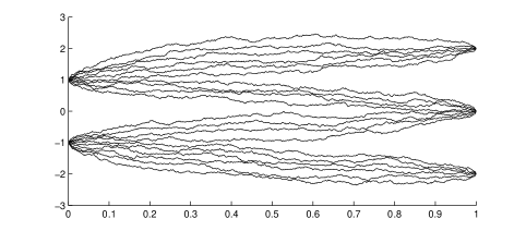
Figure 1: The figure shows $n=20$ non-intersecting Brownian motions with $p=2$ starting points and $q=3$ ending points. The horizontal axis denotes the time $t\in[0,1]$ and the vertical axis denotes the space variable $x$. For each $t\in(0,1)$ the positions $x_{1},\ldots,x_{n}$ of the paths at time $t$ form a MOP ensemble (1.10)–(1.12).

To facilitate comparison with the literature, we may note the following terminology which is often used: the MOP ensemble is said to be of type I if $q=1$, of type II if $p=1$ and of mixed type if $p,q\geq 2$. Thus the results of our paper will be valid for general MOP ensembles of mixed type, whereas the results of [5, 13, 22] only apply to MOP ensembles of type I or type II.

1.3 Riemann-Hilbert problem and kernel

The MOP ensemble in Section 1.2 and its associated multiple orthogonal polynomials are intimately related to the following Riemann-Hilbert problem (RH problem) introduced in [11]. The RH problem generalizes the well-known RH problem for orthogonal polynomials due to Fokas-Its-Kitaev [15] as well as its generalization in [29].

RH problem 1.1.

Consider the data $\mathbf{n}$, $\mathbf{w}_{1}(x)$, $\mathbf{m}$ and $\mathbf{w}_{2}(x)$ as above and assume that $|\mathbf{n}|=|\mathbf{m}|=:n$. The RH problem consists in finding a matrix-valued function $Y(z)=Y_{\mathbf{n},\mathbf{w}_{1},\mathbf{m},\mathbf{w}_{2}}(z)$ of size $p+q$ by $p+q$ such that

• $Y(z)$ is analytic in $\mathbb{C}\setminus\mathbb{R}$;

• For $x\in\mathbb{R}$, it holds that

  $$Y_{+}(x)=Y_{-}(x)\begin{pmatrix}I_{p}&W(x)\\ 0&I_{q}\end{pmatrix},$$ (1.13)

  where $I_{k}$ denotes the identity matrix of size $k$; where

  $$W(x)=\begin{pmatrix}w_{1,1}(x)w_{2,1}(x)&\ldots&w_{1,1}(x)w_{2,q}(x)\\ \vdots&&\vdots\\ w_{1,p}(x)w_{2,1}(x)&\ldots&w_{1,p}(x)w_{2,q}(x)\end{pmatrix}=\begin{pmatrix}w_{1,1}(x)\\ \vdots\\ w_{1,p}(x)\end{pmatrix}\begin{pmatrix}w_{2,1}(x)&\ldots&w_{2,q}(x)\end{pmatrix},$$ (1.14)

  and where the notation $Y_{+}(x),Y_{-}(x)$ denotes the limit of $Y(z)$ with $z$ approaching $x\in\mathbb{R}$ from the upper or lower half plane in $\mathbb{C}$, respectively;

• As $z\to\infty$, we have that

  $$Y(z)=(I_{p+q}+O(1/z))\operatorname{diag}(z^{n_{1}},\ldots,z^{n_{p}},z^{-m_{1}},\ldots,z^{-m_{q}}).$$ (1.15)

The solution $Y(z)$ to the RH problem is unique, if it exists. Partition this matrix as

$$Y(z)=\begin{array}[]{ll}&\begin{array}[]{ll}\ \ \ \ p&\ \ \ \ \ \ \ \ q\end{array}\\ \begin{array}[]{l}p\\ q\end{array}&\begin{pmatrix}Y_{1,1}(z)&Y_{1,2}(z)\\ Y_{2,1}(z)&Y_{2,2}(z)\end{pmatrix},\end{array}$$ (1.16)

where the partition is such that $Y_{1,1}(z)$ has size $p\times p$, and so on. Then the entries of $Y_{1,1}$ and $Y_{2,1}$ can be described in terms of multiple orthogonal polynomials, while $Y_{1,2}$ and $Y_{2,2}$ contain certain Cauchy transforms thereof; see Section 2 for details.

The RH problem can be used to define the Christoffel-Darboux kernel. There are actually two kernels into play. The first is a $q\times p$ matrix-valued kernel $K_{n}(x,y)$ defined as

$$K_{n}(x,y)=\frac{1}{2\pi i(y-x)}\begin{pmatrix}0&I_{q}\end{pmatrix}Y^{-1}(x)Y(y)\begin{pmatrix}I_{p}\\ 0\end{pmatrix},$$ (1.17)

for $x,y\in\mathbb{C}$, $x\neq y$. This definition may seem rather unmotivated; but see Section 2 for the connection with the classical definition of the Christoffel-Darboux kernel.

Second, there is also a scalar-valued kernel $\hat{K}_{n}(x,y)$ defined by

$$\hat{K}_{n}(x,y)=\begin{pmatrix}w_{2,1}(x)&\ldots&w_{2,q}(x)\end{pmatrix}K_{n}(x,y)\begin{pmatrix}w_{1,1}(y)\\ \vdots\\ w_{1,p}(y)\end{pmatrix}.$$ (1.18)

It is known that the MOP ensemble in Section 1.2 is determinantal with correlation kernel $\hat{K}_{n}(x,y)$ [11]. In this paper, however, the quantity of interest will be the matrix-valued kernel $K_{n}(x,y)$.

1.4 Statement of results

Now we are ready to state our main results. Throughout this section we assume fixed data $\mathbf{n}$, $\mathbf{w}_{1}(x)$, $\mathbf{m}$ and $\mathbf{w}_{2}(x)$ as before, and we consider the corresponding MOP ensemble (1.10)–(1.12). For any $K,L\in\mathbb{N}$ we define $P_{n}^{[K,L]}$ as

$$P_{n}^{[K,L]}(y_{1},\ldots,y_{K};z_{1},\ldots,z_{L}):=\\ \frac{1}{Z_{n}}\int_{-\infty}^{\infty}\ldots\int_{-\infty}^{\infty}\frac{\prod_{k=1}^{K}\left(\prod_{j=1}^{n}(y_{k}-x_{j})\right)}{\prod_{k=1}^{L}\left(\prod_{j=1}^{n}(z_{k}-x_{j})\right)}\det\left(f_{i}(x_{j})\right)_{i,j=1}^{n}\cdot\det\left(g_{i}(x_{j})\right)_{i,j=1}^{n}\ dx_{1}\ldots dx_{n},$$ (1.19)

i.e., $P_{n}^{[K,L]}$ is the average with respect to the MOP ensemble (1.10)–(1.12) of the ratio of products of characteristic polynomials. Here we assume that $y_{1},\ldots,y_{K}\in\mathbb{C}$, $z_{1},\ldots,z_{L}\in\mathbb{C}\setminus\mathbb{R}$ and the numbers in the set $(y_{1},\ldots,y_{K}$, $z_{1},\ldots,z_{L})$ are pairwise distinct.

Note that for $K=1$ and $L=0$, (1.19) reduces to the average characteristic polynomial (1.5), while for $K=0$ and $L=1$ it reduces to the average inverse characteristic polynomial (1.7). These are the cases under consideration in our first two main theorems.

Theorem 1.2.

(Average characteristic polynomial) We have that

$$P^{[1,0]}_{n}(y)=\det Y_{1,1}(y),$$ (1.20)

according to the partition (1.16).

Theorem 1.3.

(Average inverse characteristic polynomial) We have that

$$P_{n}^{[0,1]}(z)=\det Y_{2,2}(z),$$ (1.21)

according to the partition (1.16).

The proofs of Theorems 1.2–1.3 will be given in Section 3.2.

Remark 1.4.

• One may understand Theorem 1.2 as follows. The quantity $\det Y_{1,1}(y)$ is a monic polynomial of degree $n$, and its zeros determine the ‘typical’ point configuration of the MOP ensemble in Section 1.2. By specializing this to the MOP ensembles in the introduction, one obtains the typical eigenvalue configuration of random matrices with external source, the typical positions of non-intersecting Brownian motions, etc. However, one should be careful with these interpretations. For one thing, we do not even now if all the zeros of $\det Y_{1,1}(y)$ are real. This is an open problem.

• The functions $P_{n}^{[K,L]}$ in (1.19) are clearly invariant under the involution $(\mathbf{n},\mathbf{w}_{1})\leftrightarrow(\mathbf{m},\mathbf{w}_{2})$. The similar fact for the right hand sides of (1.20) and (1.21) is discussed in Section 2, see (2.12)–(2.13).

As we mentioned before, Theorem 1.2 generalizes a classical result for orthogonal polynomials, see e.g. [12], as well as its generalization to type II MOP due to Bleher-Kuijlaars [5]. On the other hand, Theorem 1.3 generalizes a result for orthogonal polynomials due to Fyodorov-Strahov [16], and also its generalization to type I MOP due to Desrosiers-Forrester [13], see also [22].

Now we state our third main theorem.

Theorem 1.5.

(Average ratio of characteristic polynomials) For the case where $K=L=1$ in (1.19), we have that

$$P_{n}^{[1,1]}(y,z)=\det L_{n}(y,z)$$ (1.22)

where $L_{n}$ is the $q$ by $q$ matrix

$$L_{n}(y,z):=I_{q}-(z-y)\int_{-\infty}^{\infty}K_{n}(y,x)W(x)/(z-x)\ dx=\begin{pmatrix}0&I_{q}\end{pmatrix}Y^{-1}(y)Y(z)\begin{pmatrix}0\\ I_{q}\end{pmatrix}.$$ (1.23)

Alternatively, we also have

$$P_{n}^{[1,1]}(y,z)=\det R_{n}(z,y)$$ (1.24)

where $R_{n}$ is the $p$ by $p$ matrix

$$R_{n}(z,y):=I_{p}-(z-y)\int_{-\infty}^{\infty}W(x)K_{n}(x,y)/(z-x)\ dx=\begin{pmatrix}I_{p}&0\end{pmatrix}Y^{-1}(z)Y(y)\begin{pmatrix}I_{p}\\ 0\end{pmatrix}.$$ (1.25)

Here $W(x)$ is the weight matrix (1.14) and $K_{n}(x,y)$ is the Christoffel-Darboux kernel (1.17).

The proof of Theorem 1.5 will be given in Section 3.1.

Note that the matrices $W(x)$ and $K_{n}(x,y)$ are of size $p\times q$ and $q\times p$, respectively, so each of the matrix expressions in (1.23) and (1.25) is well-defined. (The integrals are taken entry-wise.) The equalities between these expressions are discussed in Section 2.5.

Corollary 1.6.

Assume that $q=1$ and $w_{2,1}(x)\equiv 1$. Then

$$P_{n}^{[1,1]}(y,z)=1-(z-y)\int_{-\infty}^{\infty}\hat{K}_{n}(y,x)/(z-x)\ dx,$$ (1.26)

where $\hat{K}_{n}$ is the scalar kernel in (1.18). In particular,

$$\hat{K}_{n}(y,z)=\frac{1}{z-y}\lim_{\epsilon\to 0}\frac{1}{2\pi i}\left(P_{n}^{[1,1]}(y,z+\epsilon i)-P_{n}^{[1,1]}(y,z-\epsilon i)\right),\qquad z\in\mathbb{R}.$$ (1.27)

Similar results hold when $p=1$ and $w_{1,1}(x)\equiv 1$.

Formula (1.27) retrieves a result in [13], see also [7] for the scalar case $p=q=1$.

Finally, let us consider the case of arbitrary $K$ and $L$ in (1.19). To this end we need some extra notation.

Definition 1.7.

Assume that $|\mathbf{n}|=|\mathbf{m}|$. We set $(\mathbf{n}_{0},\mathbf{m}_{0}):=(\mathbf{n},\mathbf{m})$ and we define the sequence of multi-indices $(\mathbf{n}_{k},\mathbf{m}_{k})$, each $\mathbf{n}_{k}$ being a vector of length $p$ and each $\mathbf{m}_{k}$ a vector of length $q$, for $k\in\mathbb{Z}$ inductively as follows

• For $k=1,2,\ldots$, we set $\mathbf{n}_{k}:=\mathbf{n}_{k-1}+(1,1,\ldots,1)$ and we fix $\mathbf{m}_{k}$ arbitrarily such that $\mathbf{m}_{k}\geq\mathbf{m}_{k-1}$ componentwise and $|\mathbf{m}_{k}-\mathbf{m}_{k-1}|=p$.

• For $k=-1,-2,\ldots$, we set $\mathbf{m}_{k}:=\mathbf{m}_{k+1}-(1,1,\ldots,1)$ and we fix $\mathbf{n}_{k}$ arbitrarily such that $\mathbf{n}_{k}\leq\mathbf{n}_{k+1}$ componentwise and $|\mathbf{n}_{k+1}-\mathbf{n}_{k}|=q$.

Definition 1.7 implies that $|\mathbf{n}_{k}|=|\mathbf{m}_{k}|$ for each $k$, so we can consider the RH problem with respect to the pair of multi-indices $(\mathbf{n}_{k},\mathbf{m}_{k})$. We will assume that the RH problem is solvable for all involved pairs of multi-indices.

Note that in Definition 1.7 the multi-indices $(\mathbf{n}_{k},\mathbf{m}_{k})$ for negative $k$ are only meaningful provided $|k|\leq\min_{l=1,\ldots,q}m_{l}$. Otherwise we would obtain multi-indices with negative components.

Now we are ready to consider (1.19) for arbitrary $K$ and $L$. It turns out that the results can be expressed as determinants of large matrices constructed from the ‘building blocks’ in Theorems 1.2–1.5. To get the idea we first describe the three typical cases.

Theorem 1.8.

For the expression $P_{n}^{[K,L]}$ in (1.19), we have

• If $L=0$ then

  $$P_{n}^{[K,0]}(y_{1},\ldots,y_{K})=\frac{1}{\prod_{1\leq i<j\leq K}(y_{j}-y_{i})^{p}}\det\begin{pmatrix}(Y_{1,1})_{\mathbf{n}_{0},\mathbf{m}_{0}}(y_{1})&\ldots&(Y_{1,1})_{\mathbf{n}_{0},\mathbf{m}_{0}}(y_{K})\\ \vdots&&\vdots\\ (Y_{1,1})_{\mathbf{n}_{K-1},\mathbf{m}_{K-1}}(y_{1})&\ldots&(Y_{1,1})_{\mathbf{n}_{K-1},\mathbf{m}_{K-1}}(y_{K})\end{pmatrix}.$$ (1.28)

• If $K=0$ then

  $$P_{n}^{[0,L]}(z_{1},\ldots,z_{L})=\frac{1}{\prod_{1\leq i<j\leq L}(z_{j}-z_{i})^{q}}\det\begin{pmatrix}(Y_{2,2})_{\mathbf{n}_{0},\mathbf{m}_{0}}(z_{1})&\ldots&(Y_{2,2})_{\mathbf{n}_{0},\mathbf{m}_{0}}(z_{L})\\ \vdots&&\vdots\\ (Y_{2,2})_{\mathbf{n}_{-(L-1)},\mathbf{m}_{-(L-1)}}(z_{1})&\ldots&(Y_{2,2})_{\mathbf{n}_{-(L-1)},\mathbf{m}_{-(L-1)}}(z_{L})\end{pmatrix}.$$ (1.29)

  Here we assume that $L\leq 1+\min_{l=1}^{q}m_{l}$.

• If $K=L$ then

  $$P_{n}^{[K,K]}(y_{1},\ldots,y_{K},z_{1},\ldots,z_{K})\\ =\left(\frac{\prod_{i,j=1}^{K}(z_{j}-y_{i})}{\prod_{1\leq i<j\leq K}(y_{j}-y_{i})(z_{i}-z_{j})}\right)^{p}\det\begin{pmatrix}\frac{1}{z_{1}-y_{1}}R_{n}(z_{1},y_{1})&\ldots&\frac{1}{z_{1}-y_{K}}R_{n}(z_{1},y_{K})\\ \vdots&&\vdots\\ \frac{1}{z_{K}-y_{1}}R_{n}(z_{K},y_{1})&\ldots&\frac{1}{z_{K}-y_{K}}R_{n}(z_{K},y_{K})\end{pmatrix},$$ (1.30)

  where $R_{n}$ is the matrix in (1.25). A similar result holds with the matrix $L_{n}$ in (1.23).

Theorem 1.8 generalizes results for the scalar case in [16]. Our proof will be based on the methods of [4].

We note that Parts (a)–(b) of Theorem 1.8 are of a different flavor than Part (c). In fact, it is shown in [4, 16] that in the scalar case, one can obtain ‘mixtures’ of the formulas in Parts (a)–(b); but these formulas do not seem to have an analogue in the present setting. This is the reason why we need to work with the formula of ‘two-point’ type in Part (c).

The case of arbitrary $K,L$ in (1.19) is obtained from mixtures of either Parts (a) and (c), or Parts (b) and (c) of Theorem 1.8.

Theorem 1.9.

For the expression $P_{n}^{[K,L]}$ in (1.19), we have

• If $K\geq L$ then

  $$P_{n}^{[K,L]}(y_{1},\ldots,y_{K},z_{1},\ldots,z_{L})=\left(\frac{(-1)^{L(K-L)}\prod_{i,j}(z_{j}-y_{i})}{\prod_{1\leq i<j\leq K}(y_{j}-y_{i})\prod_{1\leq i<j\leq L}(z_{i}-z_{j})}\right)^{p}\times\\ \det\begin{pmatrix}\frac{1}{z_{1}-y_{1}}R_{n}(z_{1},y_{1})&\ldots&\frac{1}{z_{1}-y_{K}}R_{n}(z_{1},y_{K})\\ \vdots&&\vdots\\ \frac{1}{z_{L}-y_{1}}R_{n}(z_{L},y_{1})&\ldots&\frac{1}{z_{L}-y_{K}}R_{n}(z_{L},y_{K})\\ (Y_{1,1})_{\mathbf{n}_{0},\mathbf{m}_{0}}(y_{1})&\ldots&(Y_{1,1})_{\mathbf{n}_{0},\mathbf{m}_{0}}(y_{K})\\ \vdots&&\vdots\\ (Y_{1,1})_{\mathbf{n}_{K-L-1},\mathbf{m}_{K-L-1}}(y_{1})&\ldots&(Y_{1,1})_{\mathbf{n}_{K-L-1},\mathbf{m}_{K-L-1}}(y_{K})\end{pmatrix}.$$ (1.31)

  Here all $R_{n}$ matrices are taken with respect to the pair of multi-indices $\mathbf{n}_{0},\mathbf{m}_{0}$.

• If $L\geq K$ then

  $$P_{n}^{[K,L]}(y_{1},\ldots,y_{K},z_{1},\ldots,z_{L})=\left(\frac{\prod_{i,j}(z_{j}-y_{i})}{\prod_{1\leq i<j\leq K}(y_{i}-y_{j})\prod_{1\leq i<j\leq L}(z_{j}-z_{i})}\right)^{q}\times\\ \det\begin{pmatrix}\frac{1}{z_{1}-y_{1}}L_{n}(y_{1},z_{1})&\ldots&\frac{1}{z_{L}-y_{1}}L_{n}(y_{1},z_{L})\\ \vdots&&\vdots\\ \frac{1}{z_{1}-y_{K}}L_{n}(y_{K},z_{1})&\ldots&\frac{1}{z_{L}-y_{K}}L_{n}(y_{K},z_{L})\\ (Y_{2,2})_{\mathbf{n}_{0},\mathbf{m}_{0}}(z_{1})&\ldots&(Y_{2,2})_{\mathbf{n}_{0},\mathbf{m}_{0}}(z_{L})\\ \vdots&&\vdots\\ (Y_{2,2})_{\mathbf{n}_{-(L-K-1)},\mathbf{m}_{-(L-K-1)}}(z_{1})&\ldots&(Y_{2,2})_{\mathbf{n}_{-(L-K-1)},\mathbf{m}_{-(L-K-1)}}(z_{L})\end{pmatrix}.$$ (1.32)

  Here all $L_{n}$ matrices are taken with respect to the pair of multi-indices $\mathbf{n}_{0},\mathbf{m}_{0}$, and we assume that $L-K\leq 1+\min_{l=1}^{q}m_{l}$.

1.5 About the proofs of Theorems 1.5 and 1.8(c)

Theorems 1.5 and 1.8(c) will be the key results from which all other main theorems will follow. The proofs of these two theorems will be based on a Schur complement formula for the kernel $K_{n}(x,y)$. This formula is valid for an arbitrary weight matrix

$$W(x)=\begin{pmatrix}W_{k,l}(x)\end{pmatrix}_{k=1,\ldots,p,l=1,\ldots,q}$$ (1.33)

of size $p$ by $q$. Thus $W(x)$ does not need to have the rank-one factorization (1.14). For any $k\in\{1,\ldots,p\}$ and $l\in\{1,\ldots,q\}$ let

$$\mu_{j}^{(k,l)}=\int_{-\infty}^{\infty}x^{j}W_{k,l}(x)\ dx\in\mathbb{R}$$

denote the $j$th moment of the weight function $W_{k,l}(x)$, and for any $r,s\in\mathbb{N}$ let

$$H^{(k,l)}_{r,s}=\begin{pmatrix}\mu^{(k,l)}_{i+j}\end{pmatrix}_{i=0,\ldots,r-1,j=0,\ldots,s-1}$$

be the $r\times s$ Hankel matrix formed out of these moments. Stack these matrices in the block Hankel matrix

$$H_{\mathbf{n},\mathbf{m}}=\begin{pmatrix}H^{(1,1)}_{n_{1},m_{1}}&\ldots&H^{(1,q)}_{n_{1},m_{q}}\\ \vdots&&\vdots\\ H^{(p,1)}_{n_{p},m_{1}}&\ldots&H^{(p,q)}_{n_{p},m_{q}}\end{pmatrix}.$$ (1.34)

Note that this matrix is of size $n\times n$.

Recall that for a block matrix

$$M:=\begin{pmatrix}A&B\\ C&D\end{pmatrix}$$ (1.35)

with $A$ square of size $k\times k$ (say), the Schur complement of $M$ with respect to the submatrix $D$ is defined as the matrix

$$S_{M,D}:=D-CA^{-1}B,$$ (1.36)

provided $A$ is invertible. Schur complements are also known as quasi-determinants in the literature [18]. For more information on Schur complements see Section 1.6.

Proposition 1.10.

The kernel $K_{n}(x,y)$ equals the Schur complement of the matrix

$$-\left(\begin{array}[]{ccc|ccc}H_{n_{1},m_{1}}^{(1,1)}&\ldots&H_{n_{1},m_{q}}^{(1,q)}&\mathbf{y}_{n_{1}}&&\mathbf{0}\\ \vdots&&\vdots&&\ddots&\\ H_{n_{p},m_{1}}^{(p,1)}&\ldots&H_{n_{p},m_{q}}^{(p,q)}&\mathbf{0}&&\mathbf{y}_{n_{p}}\\ \hline\cr\vphantom{\overset{O}{\sim}}\mathbf{x}_{m_{1}}^{T}&&\mathbf{0}&0&\ldots&0\\ &\ddots&&\vdots&&\vdots\\ \mathbf{0}&&\mathbf{x}_{m_{q}}^{T}&0&\ldots&0\end{array}\right)$$ (1.37)

with respect to its bottom right $q\times p$ submatrix. Here the superscript ^T denotes the matrix transpose, and we use the column vector notations $\mathbf{y}_{m}=\begin{pmatrix}1&y&\ldots&y^{m-1}\end{pmatrix}^{T}$ and $\mathbf{x}_{m}=\begin{pmatrix}1&x&\ldots&x^{m-1}\end{pmatrix}^{T}$.

Proposition 1.10 will be proved in Section 2.5. Variants of this proposition in different contexts can be found in [6, 23], see also [3].

Proposition 1.10 will allow the quantities $\det L_{n}(y,z)$ and $\det R_{n}(z,y)$ in Theorem 1.5 to be written as a ratio of two determinants. In Section 3.1 we will expand these determinants using an adaptation of the classical argument of Heine, and this will lead us to the proof of Theorem 1.5. In Section 3.3 we will give a similar argument proving Theorem 1.8(c).

1.6 Background on Schur complements

Since Schur complements frequently occur in this paper, we find it convenient to list here some basic properties.

Recall the setting in (1.35) and (1.36). Schur complements are related to Gaussian elimination as follows:

$$\begin{pmatrix}A&B\\ C&D\end{pmatrix}\sim\begin{pmatrix}A&0\\ 0&S_{M,D}\end{pmatrix},$$ (1.38)

where the $\sim$ symbol relates matrices that can be obtained from one another by multiplying on the left and on the right with square transformation matrices of the form $\begin{pmatrix}I_{k}&0\\ *&I\end{pmatrix}$ and $\begin{pmatrix}I_{k}&*\\ 0&I\end{pmatrix}$, respectively. The procedure to move from the left to the right hand side of (1.38) is sometimes called Gaussian elimination with pivot block $A$, see [19].

In the special case where $D$ and (hence) $S_{M,D}$ are square matrices, one obtains from (1.38) the determinant relation

$$\det S_{M,D}=\frac{\det M}{\det A}.$$ (1.39)

Let $s_{i,j}$ denote the $(i,j)$th entry of $S=S_{M,D}$. By (1.36) one has

$$s_{i,j}=d_{i,j}-\mathbf{c}_{i}A^{-1}\mathbf{b}_{j},$$ (1.40)

where $\mathbf{c}_{i}$ denotes the $i$th row of $C$ and $\mathbf{b}_{j}$ denotes the $j$th column of $B$. Now (1.40) is nothing but the Schur complement of the matrix

$$\begin{pmatrix}A&\mathbf{b}_{j}\\ \mathbf{c}_{i}&d_{i,j}\end{pmatrix}$$ (1.41)

with respect to the entry $d_{i,j}$. From (1.39) we then obtain the determinantal expression

$$s_{i,j}=\frac{\det\begin{pmatrix}A&\mathbf{b}_{j}\\ \mathbf{c}_{i}&d_{i,j}\end{pmatrix}}{\det A}.$$ (1.42)

This shows that the entries of the Schur complement are ratios of determinants.

More generally than (1.41), one may observe that Schur complements are well-behaved with respect to taking submatrices, in the sense that any submatrix of the Schur complement (1.36) is itself a Schur complement, of an appropriate submatrix of (1.35).

Finally, observe that for any matrix $U$ of appropriate size, the matrix product $US_{M,D}=U(D-CA^{-1}B)$ can again be written as a Schur complement, of the matrix

$$\begin{pmatrix}A&B\\ UC&UD\end{pmatrix}.$$ (1.43)

A similar fact holds for matrix products of the form $S_{M,D}V$.

1.7 Outline of the rest of the paper

The rest of this paper is organized as follows. In Section 2 we discuss auxiliary results and notations that are used in the proofs of the main theorems, and we prove Proposition 1.10. Theorems 1.5 and 1.8(c) are then proved in Section 3, by an adaptation of the classical argument of Heine. Theorems 1.2 and 1.3 are obtained as limiting cases of Theorem 1.5. Finally, the generalizations to arbitrary products and ratios of characteristic polynomials are proved in Section 4.

2 Preliminaries for the proofs

In this section we collect some auxiliary results and notations that are used in the proofs of the main theorems. This section is organized as follows. Vector orthogonal polynomials (which include multiple orthogonal polynomials as a special case) are defined in Section 2.1 and their relation to the RH problem in Section 2.2. The connection with block Hankel determinants and the duality relations are discussed in Sections 2.3 and 2.4. In Section 2.5 we discuss the Christoffel-Darboux kernel, leading to the proof of Proposition 1.10. Finally, the related quantities $L_{n}$ and $R_{n}$ are investigated in Section 2.6.

Remark 2.1.

Practical note: the reader who is mainly interested in Theorems 1.2, 1.3 and 1.5 and who wants to take Proposition 1.10 for granted may skip this entire section and move directly to Section 3.

2.1 Vector orthogonal polynomials

Let $p,q\in\mathbb{N}$ and consider the multi-indices $\mathbf{n},\mathbf{m}$ as in the beginning of Section 1.2, but now with $|\mathbf{n}|=|\mathbf{m}|+1$. Let $W(x)$ be a $p$ by $q$ weight matrix as in (1.33). Our definition of vector orthogonal polynomials will be the same as in Sorokin-Van Iseghem [24]; this definition includes multiple orthogonal polynomials as a special case, when the weight matrix $W(x)$ has the rank-one factorization (1.14).

Let ${\cal P}_{\mathbf{n}}$ be the following space of polynomial vectors

$${\cal P}_{\mathbf{n}}=\{\mathbf{P}(x)=\begin{pmatrix}P_{1}(x)\\ \vdots\\ P_{p}(x)\end{pmatrix}\textrm{ with $P_{k}(x)$ a polynomial of degree at most }n_{k}-1\}.$$ (2.1)

The standard basis $(\mathbf{A}_{1}(x),\ldots,\mathbf{A}_{|\mathbf{n}|}(x))$ of the vector space ${\cal P}_{\mathbf{n}}$ is defined by the column vectors of the $p$ by $|\mathbf{n}|$ matrix

$$\begin{pmatrix}\mathbf{A}_{1}(x)&\ldots&\mathbf{A}_{|\mathbf{n}|}(x)\end{pmatrix}=\left(\begin{array}[]{cccc|cccc|cc}1&x&\ldots&x^{n_{1}-1}&0&0&\ldots&0&\ldots&0\\ 0&0&\ldots&0&1&x&\ldots&x^{n_{2}-1}&\ldots&0\\ \vdots&\vdots&&\vdots&\vdots&\vdots&&\vdots&&\vdots\\ 0&0&\ldots&0&0&0&\ldots&0&\ldots&x^{n_{p}-1}\end{array}\right).$$ (2.2)

Similarly, let ${\cal P}_{\mathbf{m}}$ denote the vector space

$${\cal P}_{\mathbf{m}}=\{\mathbf{Q}(x)=\begin{pmatrix}Q_{1}(x)\\ \vdots\\ Q_{q}(x)\end{pmatrix}\textrm{ with $Q_{l}(x)$ a polynomial of degree at most }m_{l}-1\},$$ (2.3)

and define the standard basis $(\mathbf{B}_{1}(x),\ldots,\mathbf{B}_{|\mathbf{m}|}(x))$ for ${\cal P}_{\mathbf{m}}$ by the columns of the $q$ by $|\mathbf{m}|$ matrix

$$\begin{pmatrix}\mathbf{B}_{1}(x)&\ldots&\mathbf{B}_{|\mathbf{m}|}(x)\end{pmatrix}=\left(\begin{array}[]{cccc|cccc|cc}1&x&\ldots&x^{m_{1}-1}&0&0&\ldots&0&\ldots&0\\ 0&0&\ldots&0&1&x&\ldots&x^{m_{2}-1}&\ldots&0\\ \vdots&\vdots&&\vdots&\vdots&\vdots&&\vdots&&\vdots\\ 0&0&\ldots&0&0&0&\ldots&0&\ldots&x^{m_{q}-1}\end{array}\right).$$ (2.4)

Note that we use boldface notation to denote vector-valued objects.

We say that $\mathbf{P}(x)=\mathbf{P}_{\mathbf{n},\mathbf{m}}(x)\in{\cal P}_{\mathbf{n}}$ is a vector orthogonal polynomial with respect to the multi-indices $\mathbf{n}$, $\mathbf{m}$ and the weight matrix $W(x)$ if

$$\int_{-\infty}^{\infty}\mathbf{P}_{\mathbf{n},\mathbf{m}}^{T}(x)W(x)\mathbf{Q}(x)dx=0$$

for every $\mathbf{Q}\in{\cal P}_{\mathbf{m}}$. To stress the dependence on the weight matrix we will sometimes write $\mathbf{P}_{\mathbf{n},\mathbf{m}}(x)=\mathbf{P}_{\mathbf{n},\mathbf{m},W}(x)$.

The coefficients of the vector orthogonal polynomials can be found from a homogeneous linear system with $|\mathbf{n}|$ unknowns (polynomial coefficients) and $|\mathbf{m}|$ equations (orthogonality conditions). The restriction $|\mathbf{n}|=|\mathbf{m}|+1$ guarantees that this system has a nontrivial solution. If $\mathbf{P}_{\mathbf{n},\mathbf{m}}(x)$ is unique up to a multiplicative factor then the pair of multi-indices $\mathbf{n},\mathbf{m}$ is called normal.

Assume that $\mathbf{n},\mathbf{m}$ is a normal pair of indices. Then $\mathbf{P}_{\mathbf{n},\mathbf{m}}(x)$ is said to satisfy

• the normalization of type I with respect to the $l$th index, $l\in\{1,\ldots,q\}$, if

  $$\int_{-\infty}^{\infty}\mathbf{P}^{T}_{\mathbf{n},\mathbf{m}}(x)W(x)\mathbf{Q}(x)\ dx=1$$

  where $\mathbf{Q}(x)$ is the vector consisting of zeros except for the $l$th entry which is $x^{m_{l}}$.

• the normalization of type II with respect to the $k$th index, $k\in\{1,\ldots,p\}$, if the $k$th component $(P_{k})_{\mathbf{n},\mathbf{m}}(x)$ is monic, i.e., if

  $$(P_{k})_{\mathbf{n},\mathbf{m}}(x)=x^{n_{k}-1}+O(x^{n_{k}-2}).$$

The vector orthogonal polynomials $\mathbf{P}_{\mathbf{n},\mathbf{m}}(x)$ corresponding to the above normalizations, if they exist, will be denoted as $\mathbf{P}_{\mathbf{n},\mathbf{m}}^{(I,l)}(x)$ and $\mathbf{P}_{\mathbf{n},\mathbf{m}}^{(II,k)}(x)$, respectively.

2.2 Solution to the RH problem

Consider again the RH problem in Section 1.3 with $|\mathbf{n}|=|\mathbf{m}|$ but now with $W(x)$ in (1.14) replaced by an arbitrary matrix (1.33). The solution to the RH problem, if it exists, is uniquely described by vector orthogonal polynomials and their Cauchy transforms [11]. More precisely, consider again the partition of $Y(z)$ as in (1.16). Then one has that

• $Y_{1,1}(z)$ has its $k$th row given by the row vector

  $$(\mathbf{P}^{(II,k)}_{\mathbf{n}+\mathbf{e}_{k},\mathbf{m}})^{T}(z),$$ (2.5)

  $k=1,\ldots,p$.

• $Y_{2,1}(z)$ has its $l$th row given by

  $$-2\pi i(\mathbf{P}^{(I,l)}_{\mathbf{n},\mathbf{m}-\mathbf{e}_{l}})^{T}(z),$$ (2.6)

  $l=1,\ldots,q$.

• $Y_{1,2}(z)$ has its $k$th row given by

  $$-\frac{1}{2\pi i}\int_{-\infty}^{\infty}\frac{(\mathbf{P}^{(II,k)}_{\mathbf{n}+\mathbf{e}_{k},\mathbf{m}})^{T}(x)W(x)}{z-x}\ dx,$$ (2.7)

  $k=1,\ldots,p$.

• $Y_{2,2}(z)$ has its $l$th row given by

  $$\int_{-\infty}^{\infty}\frac{(\mathbf{P}^{(I,l)}_{\mathbf{n},\mathbf{m}-\mathbf{e}_{l}})^{T}(x)W(x)}{z-x}\ dx,$$ (2.8)

  $l=1,\ldots,q$.

Here we are using the notation $\mathbf{e}_{l}$ to denote the standard basis vector which is zero except for its $l$th entry which is one. The length of this vector will always be clear from the context.

For example, in the special case where $p=q=2$, the solution $Y(z)$ is given by the $4\times 4$ matrix

$$Y(z)=D\times\left(\begin{array}[]{cccc}(P_{1})_{\mathbf{n}+\mathbf{e}_{1},\mathbf{m}}^{(II,1)}&(P_{2})_{\mathbf{n}+\mathbf{e}_{1},\mathbf{m}}^{(II,1)}&*&*\\ (P_{1})_{\mathbf{n}+\mathbf{e}_{2},\mathbf{m}}^{(II,2)}&(P_{2})_{\mathbf{n}+\mathbf{e}_{2},\mathbf{m}}^{(II,2)}&*&*\\ (P_{1})_{\mathbf{n},\mathbf{m}-\mathbf{e}_{1}}^{(I,1)}&(P_{2})_{\mathbf{n},\mathbf{m}-\mathbf{e}_{1}}^{(I,1)}&*&*\\ (P_{1})_{\mathbf{n},\mathbf{m}-\mathbf{e}_{2}}^{(I,2)}&(P_{2})_{\mathbf{n},\mathbf{m}-\mathbf{e}_{2}}^{(I,2)}&*&*\\ \end{array}\right),$$

where $D:=\operatorname{diag}(1,1,-2\pi i,-2\pi i)$, and where the entries denoted with $*$ are Cauchy transforms as in (2.7) and (2.8).

2.3 Biorthogonality and moment matrix

Recall the standard bases $\mathbf{A}_{i}(x)$ and $\mathbf{B}_{j}(x)$ in (2.2) and (2.4), where now $|\mathbf{n}|=|\mathbf{m}|=:n$. The moment matrix $M$ with respect to these bases is of size $n$ by $n$ and has entries

$$M_{i,j}=\int_{-\infty}^{\infty}\mathbf{A}_{i}^{T}(x)W(x)\mathbf{B}_{j}(x)\ dx.$$

The moment matrix coincides with the block Hankel matrix $H_{\mathbf{n},\mathbf{m}}$ in (1.34).

Consider ordered bases $(\mathbf{P}_{1}(x),\ldots,\mathbf{P}_{n}(x))$ and $(\mathbf{Q}_{1}(x),\ldots,\mathbf{Q}_{n}(x))$ of the vector spaces ${\cal P}_{\mathbf{n}}$ and ${\cal P}_{\mathbf{m}}$, respectively. We say that these bases are biorthogonal if

$$\int_{-\infty}^{\infty}\mathbf{P}_{i}^{T}(x)W(x)\mathbf{Q}_{j}(x)\ dx=\delta_{i,j},$$ (2.9)

the Kronecker delta.

Lemma 2.2.

Assume that $|\mathbf{n}|=|\mathbf{m}|$. Then the following statements are equivalent

1. The RH problem for $Y(z)$ in Section 1.3 is solvable.

2. There is no non-zero vector in ${\cal P}_{\mathbf{n}}$ which is biorthogonal to the entire space ${\cal P}_{\mathbf{m}}$.

3. $\det H_{\mathbf{n},\mathbf{m}}\neq 0$.

4. There exist biorthogonal bases for the spaces ${\cal P}_{\mathbf{n}}$ and ${\cal P}_{\mathbf{m}}$.

proof. First consider the equivalence between Statements 1 and 2. Suppose that statement 2 holds true. Then each of the polynomial vectors in (2.5)–(2.6) exists [11] and therefore the RH problem for $Y(z)$ is solvable. Conversely, suppose that statement 2 does not hold. Then the polynomial vectors in (2.5)–(2.6), if they exist, are not unique and therefore the RH problem for $Y(z)$ cannot be solvable, since that would contradict the uniqueness of $Y(z)$. Finally, the equivalence between Statements 2–4 follows from standard linear algebra arguments whose description we omit. $\hfill\square\\$

2.4 Duality

The role of the biorthogonal bases $\mathbf{P}_{i}$ and $\mathbf{Q}_{j}$ is interchanged by swapping the multi-indices $\mathbf{n}$ and $\mathbf{m}$ and by transposing the weight matrix $W(x)$:

$$(\mathbf{n},\mathbf{m},W(x))\leftrightarrow(\mathbf{m},\mathbf{n},W^{T}(x)).$$ (2.10)

This duality has a nice form in terms of the RH problem [1, 11]. If we partition the RH matrices corresponding to the original and dual data in (2.10) as

$$Y_{\mathbf{n},\mathbf{m},W}=\begin{array}[]{ll}&\begin{array}[]{ll}\ \ p&\ \ \ \ q\end{array}\\ \begin{array}[]{l}p\\ q\end{array}&\begin{pmatrix}Y_{1,1}&Y_{1,2}\\ Y_{2,1}&Y_{2,2}\end{pmatrix},\end{array}\qquad Y_{\mathbf{m},\mathbf{n},W^{T}}=\begin{array}[]{ll}&\begin{array}[]{ll}\ \ q&\ \ \ \ p\end{array}\\ \begin{array}[]{l}q\\ p\end{array}&\begin{pmatrix}\tilde{Y}_{1,1}&\tilde{Y}_{1,2}\\ \tilde{Y}_{2,1}&\tilde{Y}_{2,2}\end{pmatrix},\end{array}$$

respectively, then it holds that

$$\begin{pmatrix}\tilde{Y}_{1,1}&\tilde{Y}_{1,2}\\ \tilde{Y}_{2,1}&\tilde{Y}_{2,2}\end{pmatrix}=\begin{pmatrix}Y_{2,2}&-Y_{2,1}\\ -Y_{1,2}&Y_{1,1}\end{pmatrix}^{-T},$$ (2.11)

where the superscript ^-T denotes the inverse transpose. From a well-known theorem on minors of the inverse matrix, see e.g. [17, page. 21, eq. (33)], and the general fact that $\det Y(z)\equiv 1$ it then follows that

$$\det\tilde{Y}_{1,1}(y)=\det Y_{1,1}(y)$$ (2.12)

and

$$\det\tilde{Y}_{2,2}(z)=\det Y_{2,2}(z).$$ (2.13)

The duality relations (2.12)–(2.13) take care of a point made earlier, see the remark after the statement of Theorem 1.3.

From another application of [17, loc. cit.] it also follows that

$$\det\left(\begin{pmatrix}I_{p}&0\end{pmatrix}Y^{-1}(z)Y(y)\begin{pmatrix}I_{p}\\ 0\end{pmatrix}\right)=\det\left(\begin{pmatrix}0&I_{q}\end{pmatrix}Y^{-1}(y)Y(z)\begin{pmatrix}0\\ I_{q}\end{pmatrix}\right).$$ (2.14)

Comparing this with (1.23) and (1.25), this establishes the fact that $\det R_{n}(z,y)=\det L_{n}(y,z)$, which is of course implicit in the statement of Theorem 1.5.

2.5 The Christoffel-Darboux kernel

In this section we prove the Schur complement formula for the kernel $K_{n}(x,y)$ in Proposition 1.10. To this end we identify $K_{n}(x,y)$ as a reproducing kernel. In this way we will show that (1.17) corresponds to the kernels familiar from the theory of matrix orthogonal polynomials [23] and vector orthogonal polynomials [24].

We will assume throughout that the RH problem for $Y(z)$ is solvable, which is of course necessary in order for (1.17) to make sense.

Lemma 2.3.

The kernel $K_{n}(x,y)$ is a $q\times p$ matrix whose $(i,j)$ entry is a bivariate polynomial of degree at most $m_{i}-1$ in $x$ and $n_{j}-1$ in $y$. Equivalently,

$$K_{n}(x,y)=\sum_{i,j=1}^{n}c_{i,j}\mathbf{B}_{i}(x)\mathbf{A}^{T}_{j}(y),$$ (2.15)

for certain $c_{i,j}$, where $\mathbf{A}_{j}$ and $\mathbf{B}_{i}$ denote the basis vectors in (2.2) and (2.4).

proof. The expression $\begin{pmatrix}0&I_{q}\end{pmatrix}Y^{-1}(x)Y(y)\begin{pmatrix}I_{p}\\ 0\end{pmatrix}$ in the numerator of (1.17) is made out of the polynomial entries of the matrices $Y^{-1}(x)$ and $Y(y)$, cf. (2.5)–(2.6) and (2.11). Since this expression vanishes if $x=y$, each of these polynomials is divisible by $y-x$, so the denominator of (1.17) can be divided out.$\hfill\square\\$

It was shown in [11] that for a rank-one weight matrix $W(x)$ as in (1.14), the scalar-valued kernel $\hat{K}_{n}(x,y)$ in (1.18) has a certain reproducing property. We now obtain a similar property for the matrix-valued kernel $K_{n}(x,y)$ (without restrictions on $W(x)$).

Proposition 2.4.

The kernel $K_{n}$ satisfies the reproducing property

$$\int_{-\infty}^{\infty}K_{n}(x,y)W(y)\mathbf{Q}(y)\ dy=\mathbf{Q}(x)$$ (2.16)

for any $x\in\mathbb{C}$ and $\mathbf{Q}\in{\cal P}_{\mathbf{m}}$. Moreover, this reproducing property uniquely characterizes $K_{n}(x,y)$ in the class of bivariate polynomial matrices of the form (2.15).

proof. First we establish (2.16). This can be done by adapting the proof in [11]. However, we give a more streamlined proof. We have

$$\int K_{n}(x,y)W(y)\mathbf{Q}(y)\ dy=\int K_{n}(x,y)W(y)(\mathbf{Q}(y)-\mathbf{Q}(x))\ dy+\int K_{n}(x,y)W(y)\mathbf{Q}(x)\ dy.$$

By inserting (1.17) this becomes

$$=\begin{pmatrix}0&I_{q}\end{pmatrix}Y^{-1}(x)\begin{pmatrix}\frac{1}{2\pi i}\int Y_{1,1}(y)W(y)\frac{\mathbf{Q}(y)-\mathbf{Q}(x)}{y-x}\ dy\\ \frac{1}{2\pi i}\int Y_{2,1}(y)W(y)\frac{\mathbf{Q}(y)-\mathbf{Q}(x)}{y-x}\ dy\end{pmatrix}+\begin{pmatrix}0&I_{q}\end{pmatrix}Y^{-1}(x)\begin{pmatrix}\frac{1}{2\pi i}\int\frac{Y_{1,1}(y)W(y)}{y-x}\ dy\\ \frac{1}{2\pi i}\int\frac{Y_{2,1}(y)W(y)}{y-x}\ dy\end{pmatrix}\mathbf{Q}(x).$$ (2.17)

The first term in (2.17) is zero since $\frac{\mathbf{Q}(y)-\mathbf{Q}(x)}{y-x}$ is a polynomial vector in $y$ whose $l$th entry has degree at most $m_{l}-2$, $l=1,\ldots,q$, and by invoking the orthogonality relations of the vector orthogonal polynomials. For the second term in (2.17), we recognize the defining relations for the Cauchy transforms in the second block column of the RH problem, see (2.7)–(2.8), so we get

$$=\begin{pmatrix}0&I_{q}\end{pmatrix}Y^{-1}(x)\begin{pmatrix}Y_{1,2}(x)\\ Y_{2,2}(x)\end{pmatrix}\mathbf{Q}(x)=\begin{pmatrix}0&I_{q}\end{pmatrix}\begin{pmatrix}0\\ I_{q}\end{pmatrix}\mathbf{Q}(x)=\mathbf{Q}(x).$$

This establishes (2.16) when $x\in\mathbb{C}\setminus\mathbb{R}$; the case where $x\in\mathbb{R}$ follows by continuity.

Next we show that the reproducing property (2.16) uniquely characterizes $K_{n}(x,y)$ in the class of bivariate polynomial matrices (2.15). By Lemma 2.2, $1\Rightarrow 4$, we can choose biorthogonal bases for the polynomial vector spaces ${\cal P}_{\mathbf{n}}$ and ${\cal P}_{\mathbf{m}}$; let $(\mathbf{P}_{k})_{k=1}^{n}$ and $(\mathbf{Q}_{k})_{k=1}^{n}$ be such bases. Any $q$ by $p$ matrix $M_{n}(x,y)$ of the form (2.15) can be rewritten as

$$M_{n}(x,y)=\sum_{i,j=1}^{n}\tilde{c}_{i,j}\mathbf{Q}_{i}(x)\mathbf{P}^{T}_{j}(y)$$

for suitable constants $\tilde{c}_{i,j}$. But then the reproducing property (2.16) and the biorthogonality relations (2.9) imply that $\tilde{c}_{i,j}=\delta_{i,j}$, the Kronecker delta. This ends the proof. $\hfill\square\\$

Proposition 2.4 has the following dual version.

Proposition 2.5.

The kernel $K_{n}$ satisfies the reproducing property

$$\int_{-\infty}^{\infty}\mathbf{P}^{T}(x)W(x)K_{n}(x,y)\ dx=\mathbf{P}^{T}(y)$$ (2.18)

for any $y\in\mathbb{C}$ and $\mathbf{P}\in{\cal P}_{\mathbf{n}}$. Moreover, this reproducing property uniquely characterizes $K_{n}(x,y)$ in the class of bivariate polynomial matrices of the form (2.15).

Now we are ready for the

Proof of Proposition 1.10. Denote with $M_{n}(x,y)$ the Schur complement of (1.37). We check the reproducing kernel property

$$\int\mathbf{A}^{T}(x)W(x)M_{n}(x,y)\ dx=\mathbf{A}^{T}(y),$$ (2.19)

for each column vector of the form $\mathbf{A}(x)=\begin{pmatrix}0&\ldots&x^{i_{k}}&\ldots&0\end{pmatrix}^{T}$ with $i_{k}\in\{0,\ldots,n_{k}-1\}$, $k\in\{1,\ldots,p\}$. (These vectors $\mathbf{A}(x)$ are the standard basis of the space ${\cal P}_{\mathbf{n}}$.) By using the multiplication property (1.43) for Schur complements, the left hand side of (2.19) equals the Schur complement of

$$-\left(\begin{array}[]{ccc|ccc}H_{n_{1},m_{1}}^{(1,1)}&\ldots&H_{n_{1},m_{q}}^{(1,q)}&\mathbf{y}_{n_{1}}&&\mathbf{0}\\ \vdots&&\vdots&&\ddots&\\ H_{n_{p},m_{1}}^{(p,1)}&\ldots&H_{n_{p},m_{q}}^{(p,q)}&\mathbf{0}&&\mathbf{y}_{n_{p}}\\ \hline\cr\vphantom{\overset{O}{\sim}}\mathbf{h}_{i_{k},m_{1}}^{(k,1)}&&\mathbf{h}_{i_{k},m_{q}}^{(k,q)}&0&\ldots&0\end{array}\right)$$ (2.20)

with respect to its bottom right $1\times p$ submatrix, where we use the row vector notation $\mathbf{h}_{i_{k},m_{l}}^{(k,l)}=\begin{pmatrix}\mu^{(k,l)}_{i_{k}+j}\end{pmatrix}_{j=0,\ldots,m_{l}-1}$. Subtracting from the last row of (2.20) the $i_{k}$th row from the $k$th block row, we are led to the Schur complement of

$$-\left(\begin{array}[]{ccc|ccccc}H_{n_{1},m_{1}}^{(1,1)}&\ldots&H_{n_{1},m_{q}}^{(1,q)}&\mathbf{y}_{n_{1}}&&&&\mathbf{0}\\ \vdots&&\vdots&&&\ddots&&\\ H_{n_{p},m_{1}}^{(p,1)}&\ldots&H_{n_{p},m_{q}}^{(p,q)}&\mathbf{0}&&&&\mathbf{y}_{n_{p}}\\ \hline\cr\vphantom{\overset{O}{\sim}}\mathbf{0}&&\mathbf{0}&0&\ldots&-y^{i_{k}}&\ldots&0\end{array}\right),$$ (2.21)

where now the last row is zero except for the entry $-y^{i_{k}}$ in the $k$th column of the second block column. But clearly, the Schur complement of (2.21) is just the row vector $\mathbf{A}^{T}(y)=\begin{pmatrix}0&\ldots&y^{i_{k}}&\ldots&0\end{pmatrix}$. This establishes the reproducing kernel property (2.19).

To finish the proof of the proposition, we note that the degree structure of (1.37) implies that $M_{n}(x,y)$ has the form in (2.15). Thus the proof is ended by invoking the uniqueness part of Proposition 2.5. $\hfill\square\\$

2.6 The matrices $L_{n}$ and $R_{n}$

In this section we consider in more detail the quantities $L_{n}$ and $R_{n}$ which are derived from the kernel $K_{n}$. Let us first establish the equivalence between the two different formulae in the definition of $L_{n}$ in (1.23). From the identity $y-x=(y-z)+(z-x)$ we obtain

$$\int\frac{y-x}{z-x}K_{n}(y,x)W(x)\ dx = \int K_{n}(y,x)W(x)I_{q}\ dx+\int\frac{y-z}{z-x}K_{n}(y,x)W(x)\ dx$$ (2.22)

$$= I_{q}-(z-y)\int K_{n}(y,x)W(x)/(z-x)\ dx$$

by virtue of the reproducing property in Proposition 2.4. On the other hand, the equality

$$\int\frac{y-x}{z-x}K_{n}(y,x)W(x)\ dx=\begin{pmatrix}0&I_{q}\end{pmatrix}Y^{-1}(y)Y(z)\begin{pmatrix}0\\ I_{q}\end{pmatrix}$$

follows from (1.17) and (2.7)–(2.8). This establishes the required equality in (1.23).

The equivalence between the different formulae in (1.25) can be established similarly.

In section 4, we will need the following property of $L_{n}$.

Proposition 2.6.

The matrix $L_{n}$ in (1.23) satisfies the ‘vanishing property’

$$\int_{-\infty}^{\infty}\mathbf{P}^{T}(y)W(y)\frac{L_{n}(y,z)}{z-y}\ dy=0$$ (2.23)

for any $z\in\mathbb{C}\setminus\mathbb{R}$ and $\mathbf{P}\in{\cal P}_{\mathbf{n}}$.

proof. From the expression of $L_{n}$ in (2.22), we obtain

$$\int\mathbf{P}^{T}(y)W(y)\frac{L_{n}(y,z)}{z-y}\ dy=\int\mathbf{P}^{T}(y)\frac{W(y)}{z-y}\ dy-\int\!\int\frac{\mathbf{P}^{T}(y)W(y)K_{n}(y,x)W(x)}{z-x}\ dx\ dy$$

which is

$$=\int\mathbf{P}^{T}(y)\frac{W(y)}{z-y}\ dy-\int\left(\int\mathbf{P}^{T}(y)W(y)K_{n}(y,x)dy\right)\frac{W(x)}{z-x}dx.$$

By inserting the reproducing property this becomes

$$=\int\mathbf{P}^{T}(y)\frac{W(y)}{z-y}\ dy-\int\mathbf{P}^{T}(x)\frac{W(x)}{z-x}\ dx=0.$$

$\hfill\square\\$

Here is the dual version of Proposition 2.6.

Proposition 2.7.

The matrix $R_{n}$ in (1.25) satisfies the ‘vanishing property’

$$\int_{-\infty}^{\infty}\frac{R(z,y)}{z-y}W(y)\mathbf{Q}(y)\ dy=0$$ (2.24)

for any $z\in\mathbb{C}\setminus\mathbb{R}$ and $\mathbf{Q}\in{\cal P}_{\mathbf{m}}$.

3 Proofs, part 1

In this section we prove Theorems 1.2, 1.3, 1.5 and 1.8(c).

3.1 Proof of Theorem 1.5

First we prove Theorem 1.5. The proof of this theorem will follow by expanding the moment determinant in Proposition 1.10 in a similar way as in the classical argument of Heine.

We will restrict ourselves to the proof of (1.24); the proof of (1.22) can then be devised in a similar way, or by simply invoking (2.14). For notational convenience and to keep things readable, we give the proof for the case $p=q=2$. The case of general $p,q$ is completely similar except that it requires more notational burden.

First we expand the left hand side of (1.24). By definition, the average ratio of characteristic polynomials $P_{n}^{[1,1]}(y,z)$ is given by

$$P_{n}^{[1,1]}(y,z)=\frac{1}{Z_{n}}\int\ldots\int\prod_{j=1}^{n}\frac{y-x_{j}}{z-x_{j}}\\ \left|\begin{array}[]{ccc}w_{1,1}(x_{1})&\ldots&w_{1,1}(x_{n})\\ \vdots&&\vdots\\ x_{1}^{n_{1}-1}w_{1,1}(x_{1})&\ldots&x_{n}^{n_{1}-1}w_{1,1}(x_{n})\\ \hline\cr w_{1,2}(x_{1})&\ldots&w_{1,2}(x_{n})\\ \vdots&&\vdots\\ x_{1}^{n_{2}-1}w_{1,2}(x_{1})&\ldots&x_{n}^{n_{2}-1}w_{1,2}(x_{n})\end{array}\right|\times\left|\begin{array}[]{ccc}w_{2,1}(x_{1})&\ldots&w_{2,1}(x_{n})\\ \vdots&&\vdots\\ x_{1}^{m_{1}-1}w_{2,1}(x_{1})&\ldots&x_{n}^{m_{1}-1}w_{2,1}(x_{n})\\ \hline\cr w_{2,2}(x_{1})&\ldots&w_{2,2}(x_{n})\\ \vdots&&\vdots\\ x_{1}^{m_{2}-1}w_{2,2}(x_{1})&\ldots&x_{n}^{m_{2}-1}w_{2,2}(x_{n})\end{array}\right|\prod_{j=1}^{n}dx_{j}.$$ (3.1)

We can expand the second determinant according to the Lagrange expansion with respect to the first block row:

$$\left|\begin{array}[]{ccc}w_{2,1}(x_{1})&\ldots&w_{2,1}(x_{n})\\ \vdots&&\vdots\\ x_{1}^{m_{1}-1}w_{2,1}(x_{1})&\ldots&x_{n}^{m_{1}-1}w_{2,1}(x_{n})\\ \hline\cr w_{2,2}(x_{1})&\ldots&w_{2,2}(x_{n})\\ \vdots&&\vdots\\ x_{1}^{m_{2}-1}w_{2,2}(x_{1})&\ldots&x_{n}^{m_{2}-1}w_{2,2}(x_{n})\end{array}\right|\\ =\sum_{S}(-1)^{S}\begin{vmatrix}w_{2,1}(x_{s_{1}})&\ldots&w_{2,1}(x_{s_{m_{1}}})\\ \vdots&&\vdots\\ x_{s_{1}}^{m_{1}-1}w_{2,1}(x_{s_{1}})&\ldots&x_{s_{m_{1}}}^{m_{1}-1}w_{2,1}(x_{s_{m_{1}}})\end{vmatrix}\begin{vmatrix}w_{2,2}(x_{\bar{s}_{1}})&\ldots&w_{2,2}(x_{\bar{s}_{m_{2}}})\\ \vdots&&\vdots\\ x_{\bar{s}_{1}}^{m_{2}-1}w_{2,2}(x_{\bar{s}_{1}})&\ldots&x_{\bar{s}_{m_{2}}}^{m_{2}-1}w_{2,2}(x_{\bar{s}_{m_{2}}})\end{vmatrix}$$ (3.2)

where the sum is over all $\binom{n}{m_{1}}$ subsets $S\subset\{1,\ldots,n\}$ with $|S|=m_{1}$, where we write the elements of $S$ in increasing order: $s_{1}<\ldots<s_{m_{1}}$, similarly for those of the complement $\bar{S}=\{1,\ldots,n\}\setminus S$, $\bar{s}_{1}<\ldots<\bar{s}_{m_{2}}$, and where we denote by $(-1)^{S}$ the sign of the permutation $s_{1},\ldots,s_{m_{1}},\bar{s}_{1},\ldots,\bar{s}_{m_{2}}$.

For each term of (3.2) we can incorporate the factor $(-1)^{S}$ into the other determinant of (3.1) by permuting its columns. Next we can relabel the variables $x_{1},\ldots,x_{n}$ back in their original form, and so (3.1) reduces to

$$P_{n}^{[1,1]}(y,z)=\frac{\binom{n}{m_{1}}}{Z_{n}}\int\ldots\int\prod_{j=1}^{n}\frac{y-x_{j}}{z-x_{j}}\left|\begin{array}[]{ccc}w_{1,1}(x_{1})&\ldots&w_{1,1}(x_{n})\\ \vdots&&\vdots\\ x_{1}^{n_{1}-1}w_{1,1}(x_{1})&\ldots&x_{n}^{n_{1}-1}w_{1,1}(x_{n})\\ \hline\cr w_{1,2}(x_{1})&\ldots&w_{1,2}(x_{n})\\ \vdots&&\vdots\\ x_{1}^{n_{2}-1}w_{1,2}(x_{1})&\ldots&x_{n}^{n_{2}-1}w_{1,2}(x_{n})\end{array}\right|\\ \begin{vmatrix}w_{2,1}(x_{1})&\ldots&w_{2,1}(x_{m_{1}})\\ \vdots&&\vdots\\ x_{1}^{m_{1}-1}w_{2,1}(x_{1})&\ldots&x_{m_{1}}^{m_{1}-1}w_{2,1}(x_{m_{1}})\end{vmatrix}\begin{vmatrix}w_{2,2}(x_{m_{1}+1})&\ldots&w_{2,2}(x_{n})\\ \vdots&&\vdots\\ x_{m_{1}+1}^{m_{2}-1}w_{2,2}(x_{m_{1}+1})&\ldots&x_{n}^{m_{2}-1}w_{2,2}(x_{n})\end{vmatrix}\prod_{j=1}^{n}dx_{j}$$

which on evaluating the Vandermonde determinants becomes

$$P_{n}^{[1,1]}(y,z)=\frac{\binom{n}{m_{1}}}{Z_{n}}\int\ldots\int\ \prod_{j=1}^{n}\frac{y-x_{j}}{z-x_{j}}\ \left|\begin{array}[]{ccc}w_{1,1}(x_{1})&\ldots&w_{1,1}(x_{n})\\ \vdots&&\vdots\\ x_{1}^{n_{1}-1}w_{1,1}(x_{1})&\ldots&x_{n}^{n_{1}-1}w_{1,1}(x_{n})\\ \hline\cr w_{1,2}(x_{1})&\ldots&w_{1,2}(x_{n})\\ \vdots&&\vdots\\ x_{1}^{n_{2}-1}w_{1,2}(x_{1})&\ldots&x_{n}^{n_{2}-1}w_{1,2}(x_{n})\end{array}\right|\\ \prod_{1\leq i<j\leq m_{1}}(x_{j}-x_{i})\prod_{m_{1}+1\leq i<j\leq n}(x_{j}-x_{i})\prod_{j=1}^{m_{1}}w_{2,1}(x_{j})\prod_{j=m_{1}+1}^{n}w_{2,2}(x_{j})\prod_{j=1}^{n}dx_{j}.$$ (3.3)

Next we expand the right hand side of (1.24). We recall from Proposition 1.10 that $-K_{n}(x,y)$ is the Schur complement of the matrix

$$\left(\begin{array}[]{cc|cc}H_{n_{1},m_{1}}^{(1,1)}&H_{n_{1},m_{2}}^{(1,2)}&\mathbf{y}_{n_{1}}&\mathbf{0}\\ H_{n_{2},m_{1}}^{(2,1)}&H_{n_{2},m_{2}}^{(2,2)}&\mathbf{0}&\mathbf{y}_{n_{2}}\\ \hline\cr\vphantom{\overset{O}{\sim}}\mathbf{x}^{T}_{m_{1}}&0&0&0\\ 0&\mathbf{x}^{T}_{m_{2}}&0&0\end{array}\right).$$ (3.4)

This implies that $\frac{1}{z-y}I_{2}-\int\frac{W(x)K_{n}(x,y)}{z-x}\ dx$ is the Schur complement of the matrix

$$\left(\begin{array}[]{cc|cc}H_{n_{1},m_{1}}^{(1,1)}&H_{n_{1},m_{2}}^{(1,2)}&\mathbf{y}_{n_{1}}&\mathbf{0}\\ H_{n_{2},m_{1}}^{(2,1)}&H_{n_{2},m_{2}}^{(2,2)}&\mathbf{0}&\mathbf{y}_{n_{2}}\\ \hline\cr\vphantom{\overset{O}{\sim}}\int\mathbf{x}^{T}_{m_{1}}W_{1,1}(x)/(z-x)\ dx&\int\mathbf{x}^{T}_{m_{2}}W_{1,2}(x)/(z-x)\ dx&1/(z-y)&0\\ \int\mathbf{x}^{T}_{m_{1}}W_{2,1}(x)/(z-x)\ dx&\int\mathbf{x}^{T}_{m_{2}}W_{2,2}(x)/(z-x)\ dx&0&1/(z-y)\end{array}\right).$$ (3.5)

From (1.39) this implies the determinant representation

$$\det\left(\frac{1}{z-y}I_{2}-\int\frac{W(x)K_{n}(x,y)}{z-x}\ dx\right)\\ =\frac{1}{\kappa}\begin{vmatrix}H_{n_{1},m_{1}}^{(1,1)}&H_{n_{1},m_{2}}^{(1,2)}&\mathbf{y}_{n_{1}}&\mathbf{0}\\ H_{n_{2},m_{1}}^{(2,1)}&H_{n_{2},m_{2}}^{(2,2)}&\mathbf{0}&\mathbf{y}_{n_{2}}\\ \int\mathbf{x}_{m_{1}}^{T}W_{1,1}(x)/(z-x)\ dx&\int\mathbf{x}_{m_{2}}^{T}W_{1,2}(x)/(z-x)\ dx&1/(z-y)&0\\ \int\mathbf{x}_{m_{1}}^{T}W_{2,1}(x)/(z-x)\ dx&\int\mathbf{x}_{m_{2}}^{T}W_{2,2}(x)/(z-x)\ dx&0&1/(z-y)\end{vmatrix},$$ (3.6)

where $\kappa=\det H_{\mathbf{n},\mathbf{m}}$ is the determinant of the top left block of (3.5).

Now we expand the integral in the right hand side of (3.6). By definition, each $H_{n_{k},m_{l}}^{(k,l)}$ is a Hankel matrix whose $(i,j)$th entry is the $(i+j)$th moment with respect to the weight function $W_{k,l}(x)=w_{1,k}(x)w_{2,l}(x)$, for $k,l=1,2$:

$$(H_{n_{k},m_{l}}^{(k,l)})_{i,j}=\int x^{i+j}W_{k,l}(x)\ dx.$$ (3.7)

Note that the integration variable $x$ in (3.7) is just a ‘dummy variable’ which we can give any name we want. By choosing the same integration variable $x_{1}$ for all entries in the first column of (3.6), we can rewrite (3.6) as follows:

$$=\frac{1}{\kappa}\left|\begin{array}[]{cccc|ccc|cc}\int W_{1,1}(x_{1})\ dx_{1}&*&\ldots&*&*&\ldots&*&1&0\\ \vdots&\vdots&&\vdots&\vdots&&\vdots&\vdots&\vdots\\ \int x_{1}^{n_{1}-1}W_{1,1}(x_{1})\ dx_{1}&*&\ldots&*&*&\ldots&*&y^{n_{1}-1}&0\\ \hline\cr\int W_{2,1}(x_{1})\ dx_{1}&*&\ldots&*&*&\ldots&*&0&1\\ \vdots&\vdots&&\vdots&\vdots&&\vdots&\vdots&\vdots\\ \int x_{1}^{n_{2}-1}W_{2,1}(x_{1})\ dx_{1}&*&\ldots&*&*&\ldots&*&0&y^{n_{2}-1}\\ \hline\cr\int\frac{W_{1,1}(x_{1})}{z-x_{1}}\ dx_{1}&*&\ldots&*&*&\ldots&*&\frac{1}{z-y}&0\\ \int\frac{W_{2,1}(x_{1})}{z-x_{1}}\ dx_{1}&*&\ldots&*&*&\ldots&*&0&\frac{1}{z-y}\end{array}\right|$$

where the entries denoted with $*$ are not important at this stage of the proof. Using the multi-linearity of the determinant with respect to its first column, we can take out the integration with respect to $x_{1}$:

$$=\frac{1}{\kappa}\int\ \left|\begin{array}[]{cccc|ccc|cc}w_{1,1}(x_{1})&*&\ldots&*&*&\ldots&*&1&0\\ \vdots&\vdots&&\vdots&\vdots&&\vdots&\vdots&\vdots\\ x_{1}^{n_{1}-1}w_{1,1}(x_{1})&*&\ldots&*&*&\ldots&*&y^{n_{1}-1}&0\\ \hline\cr w_{1,2}(x_{1})&*&\ldots&*&*&\ldots&*&0&1\\ \vdots&\vdots&&\vdots&\vdots&&\vdots&\vdots&\vdots\\ x_{1}^{n_{2}-1}w_{1,2}(x_{1})&*&\ldots&*&*&\ldots&*&0&y^{n_{2}-1}\\ \hline\cr\frac{w_{1,1}(x_{1})}{z-x_{1}}&*&\ldots&*&*&\ldots&*&\frac{1}{z-y}&0\\ \frac{w_{1,2}(x_{1})}{z-x_{1}}&*&\ldots&*&*&\ldots&*&0&\frac{1}{z-y}\end{array}\right|\ w_{2,1}(x_{1})dx_{1}.$$

Here we also used that $W_{1,1}(x)=w_{1,1}(x)w_{2,1}(x)$ and $W_{2,1}(x)=w_{1,2}(x)w_{2,1}(x)$, allowing us to extract the common factor $w_{2,1}(x_{1})$ from the first column. Applying the same technique to the other columns of the first block column we obtain

$$=\frac{1}{\kappa}\int\ldots\int\ \left|\begin{array}[]{ccc|ccc|cc}w_{1,1}(x_{1})&\ldots&w_{1,1}(x_{m_{1}})&*&\ldots&*&1&0\\ \vdots&&\vdots&\vdots&&\vdots&\vdots&\vdots\\ x_{1}^{n_{1}-1}w_{1,1}(x_{1})&\ldots&x_{m_{1}}^{n_{1}-1}w_{1,1}(x_{m_{1}})&*&\ldots&*&y^{n_{1}-1}&0\\ \hline\cr w_{1,2}(x_{1})&\ldots&w_{1,2}(x_{m_{1}})&*&\ldots&*&0&1\\ \vdots&&\vdots&\vdots&&\vdots&\vdots&\vdots\\ x_{1}^{n_{2}-1}w_{1,2}(x_{1})&\ldots&x_{m_{1}}^{n_{2}-1}w_{1,2}(x_{m_{1}})&*&\ldots&*&0&y^{n_{2}-1}\\ \hline\cr\frac{w_{1,1}(x_{1})}{z-x_{1}}&\ldots&\frac{w_{1,1}(x_{m_{1}})}{z-x_{m_{1}}}&*&\ldots&*&\frac{1}{z-y}&0\\ \frac{w_{1,2}(x_{1})}{z-x_{1}}&\ldots&\frac{w_{1,2}(x_{m_{1}})}{z-x_{m_{1}}}&*&\ldots&*&0&\frac{1}{z-y}\end{array}\right|\ \prod_{j=1}^{m_{1}}\left(x_{j}^{j-1}w_{2,1}(x_{j})dx_{j}\right).$$

To get rid of the factor $\prod_{j=1}^{m_{1}}x_{j}^{j-1}$ one can apply the following well-known symmetrization trick. Sum the above expression over all permutations $x_{\sigma_{1}},\ldots,x_{\sigma_{m_{1}}}$ of $x_{1},\ldots,x_{m_{1}}$. For each term in this sum, apply a column permutation to arrange the columns of the determinant back in their original form; this releases a factor $(-1)^{\sigma}$. But then we get the expansion of a Vandermonde determinant:

$$\sum_{\sigma}(-1)^{\sigma}\prod_{j=1}^{m_{1}}x_{\sigma_{j}}^{j-1}=\prod_{1\leq i<j\leq m_{1}}(x_{j}-x_{i}).$$

So we get

$$=\frac{1}{\kappa(m_{1})!}\int\ldots\int\ \left|\begin{array}[]{ccc|ccc|cc}w_{1,1}(x_{1})&\ldots&w_{1,1}(x_{m_{1}})&*&\ldots&*&1&0\\ \vdots&&\vdots&\vdots&&\vdots&\vdots&\vdots\\ x_{1}^{n_{1}-1}w_{1,1}(x_{1})&\ldots&x_{m_{1}}^{n_{1}-1}w_{1,1}(x_{m_{1}})&*&\ldots&*&y^{n_{1}-1}&0\\ \hline\cr w_{1,2}(x_{1})&\ldots&w_{1,2}(x_{m_{1}})&*&\ldots&*&0&1\\ \vdots&&\vdots&\vdots&&\vdots&\vdots&\vdots\\ x_{1}^{n_{2}-1}w_{1,2}(x_{1})&\ldots&x_{m_{1}}^{n_{2}-1}w_{1,2}(x_{m_{1}})&*&\ldots&*&0&y^{n_{2}-1}\\ \hline\cr\frac{w_{1,1}(x_{1})}{z-x_{1}}&\ldots&\frac{w_{1,1}(x_{m_{1}})}{z-x_{m_{1}}}&*&\ldots&*&\frac{1}{z-y}&0\\ \frac{w_{1,2}(x_{1})}{z-x_{1}}&\ldots&\frac{w_{1,2}(x_{m_{1}})}{z-x_{m_{1}}}&*&\ldots&*&0&\frac{1}{z-y}\end{array}\right|\\ \prod_{1\leq i<j\leq m_{1}}(x_{j}-x_{i})\prod_{j=1}^{m_{1}}w_{2,1}(x_{j})\prod_{j=1}^{m_{1}}dx_{j}.$$

Applying the same techniques to the second block column, we find

$$=\frac{1}{\kappa(m_{1})!(m_{2})!}\int\ldots\int\ \left|\begin{array}[]{ccc|cc}w_{1,1}(x_{1})&\ldots&w_{1,1}(x_{n})&1&0\\ \vdots&&\vdots&\vdots&\vdots\\ x_{1}^{n_{1}-1}w_{1,1}(x_{1})&\ldots&x_{n}^{n_{1}-1}w_{1,1}(x_{n})&y^{n_{1}-1}&0\\ \hline\cr w_{1,2}(x_{1})&\ldots&w_{1,2}(x_{n})&0&1\\ \vdots&&\vdots&\vdots&\vdots\\ x_{1}^{n_{2}-1}w_{1,2}(x_{1})&\ldots&x_{n}^{n_{2}-1}w_{1,2}(x_{n})&0&y^{n_{2}-1}\\ \hline\cr\frac{w_{1,1}(x_{1})}{z-x_{1}}&\ldots&\frac{w_{1,1}(x_{n})}{z-x_{n}}&\frac{1}{z-y}&0\\ \frac{w_{1,2}(x_{1})}{z-x_{1}}&\ldots&\frac{w_{1,2}(x_{n})}{z-x_{n}}&0&\frac{1}{z-y}\end{array}\right|\\ \prod_{1\leq i<j\leq m_{1}}(x_{j}-x_{i})\prod_{m_{1}+1\leq i<j\leq n}(x_{j}-x_{i})\prod_{j=1}^{m_{1}}w_{2,1}(x_{j})\prod_{j=m_{1}+1}^{n}w_{2,2}(x_{j})\prod_{j=1}^{n}dx_{j}.$$ (3.8)

We claim that this can be rewritten as

$$=\frac{1}{(z-y)^{2}}\frac{1}{\kappa(m_{1})!(m_{2})!}\int\ldots\int\ \frac{\prod_{j=1}^{n}(y-x_{j})}{\prod_{j=1}^{n}(z-x_{j})}\ \left|\begin{array}[]{ccc}w_{1,1}(x_{1})&\ldots&w_{1,1}(x_{n})\\ \vdots&&\vdots\\ x_{1}^{n_{1}-1}w_{1,1}(x_{1})&\ldots&x_{n}^{n_{1}-1}w_{1,1}(x_{n})\\ \hline\cr w_{1,2}(x_{1})&\ldots&w_{1,2}(x_{n})\\ \vdots&&\vdots\\ x_{1}^{n_{2}-1}w_{1,2}(x_{1})&\ldots&x_{n}^{n_{2}-1}w_{1,2}(x_{n})\end{array}\right|\\ \prod_{1\leq i<j\leq m_{1}}(x_{j}-x_{i})\prod_{m_{1}+1\leq i<j\leq n}(x_{j}-x_{i})\prod_{j=1}^{m_{1}}w_{2,1}(x_{j})\prod_{j=m_{1}+1}^{n}w_{2,2}(x_{j})\prod_{j=1}^{n}dx_{j}.$$ (3.9)

This follows from standard determinant manipulations and the exact formula for a Cauchy-Vandermonde determinant; see the appendix.

Now up to a constant factor times $1/(z-y)^{2}$, (3.9) equals (3.3). This proves (1.24), up to a constant factor; but this constant factor must be 1 as can be seen by matching the leading terms on both sides of (1.24).

Remark 3.1.

By matching the leading constants in (3.3) and (3.9), we obtain the following expression for the normalization constant $Z_{n}$ in (1.10):

$$Z_{n}=\kappa n!$$

where we recall that $\kappa$ is the block Hankel determinant $\kappa=\det H_{\mathbf{n},\mathbf{m}}$. This identity also follows directly from a ‘generalized Cauchy-Binet identity’, see e.g. [22].

3.2 Proof of Theorems 1.2 and 1.3

Having established Theorem 1.5, Theorems 1.2 and 1.3 now follow as simple limiting cases. For Theorem 1.2 we let $z\to\infty$ in (1.24) and observe from (1.25) that

$$\det R_{n}(z,y)=\det\left(\begin{pmatrix}I_{p}&0\end{pmatrix}Y^{-1}(z)Y(y)\begin{pmatrix}I_{p}\\ 0\end{pmatrix}\right)=\det\left(\begin{pmatrix}(Y^{-1})_{1,1}(z)&(Y^{-1})_{1,2}(z)\end{pmatrix}\begin{pmatrix}Y_{1,1}(y)\\ Y_{2,1}(y)\end{pmatrix}\right)\\ =z^{-n}\det Y_{1,1}(y)+O(z^{-n-1}),$$

where in the last step we used the Cauchy-Binet identity and the asymptotics (1.15). This establishes Theorem 1.2. Theorem 1.3 can be obtained in a similar way by letting $y\to\infty$ in (1.22).

3.3 Proof of Theorem 1.8(c)

The proof that we have given for Theorem 1.5 can be extended to prove Theorem 1.8(c) as well. The key observation is that the matrix in the right hand side of (1.30) can be written in Schur complement form as well. For example, for $K=L=2$ and $p=q=2$ one has that

$$\begin{pmatrix}\frac{1}{z_{1}-y_{1}}R_{n}(z_{1},y_{1})&\frac{1}{z_{1}-y_{2}}R_{n}(z_{1},y_{2})\\ \frac{1}{z_{2}-y_{1}}R_{n}(z_{2},y_{1})&\frac{1}{z_{2}-y_{2}}R_{n}(z_{2},y_{2})\end{pmatrix}$$

is the Schur complement of the matrix.

$$\left(\begin{array}[]{cc|cccc}H_{n_{1},m_{1}}^{(1,1)}&H_{n_{1},m_{2}}^{(1,2)}&(\mathbf{y}_{1})_{n_{1}}&\mathbf{0}&(\mathbf{y}_{2})_{n_{1}}&\mathbf{0}\\ H_{n_{2},m_{1}}^{(2,1)}&H_{n_{2},m_{2}}^{(2,2)}&\mathbf{0}&(\mathbf{y_{1}})_{n_{2}}&\mathbf{0}&(\mathbf{y_{2}})_{n_{2}}\\ \hline\cr\vphantom{\overset{O}{\sim}}\int\mathbf{x}^{T}_{m_{1}}W_{1,1}(x)/(z_{1}-x)\ dx&\int\mathbf{x}^{T}_{m_{2}}W_{1,2}(x)/(z_{1}-x)\ dx&1/(z_{1}-y_{1})&0&1/(z_{1}-y_{2})&0\\ \int\mathbf{x}^{T}_{m_{1}}W_{2,1}(x)/(z_{1}-x)\ dx&\int\mathbf{x}^{T}_{m_{2}}W_{2,2}(x)/(z_{1}-x)\ dx&0&1/(z_{1}-y_{1})&0&1/(z_{1}-y_{2})\\ \int\mathbf{x}^{T}_{m_{1}}W_{1,1}(x)/(z_{2}-x)\ dx&\int\mathbf{x}^{T}_{m_{2}}W_{1,2}(x)/(z_{2}-x)\ dx&1/(z_{2}-y_{1})&0&1/(z_{2}-y_{2})&0\\ \int\mathbf{x}^{T}_{m_{1}}W_{2,1}(x)/(z_{2}-x)\ dx&\int\mathbf{x}^{T}_{m_{2}}W_{2,2}(x)/(z_{2}-x)\ dx&0&1/(z_{2}-y_{1})&0&1/(z_{2}-y_{2})\end{array}\right).$$ (3.10)

Compare with (3.5).

The determinant of this Schur complement can be manipulated in the same way as in Section 3.1. This leads to the following analogue of (3.8):

$$\frac{1}{\kappa(m_{1})!(m_{2})!}\int\ldots\int\ \left|\begin{array}[]{ccc|cccc}w_{1,1}(x_{1})&\ldots&w_{1,1}(x_{n})&1&0&1&0\\ \vdots&&\vdots&\vdots&\vdots&\vdots&\vdots\\ x_{1}^{n_{1}-1}w_{1,1}(x_{1})&\ldots&x_{n}^{n_{1}-1}w_{1,1}(x_{n})&y_{1}^{n_{1}-1}&0&y_{2}^{n_{1}-1}&0\\ \hline\cr w_{1,2}(x_{1})&\ldots&w_{1,2}(x_{n})&0&1&0&1\\ \vdots&&\vdots&\vdots&\vdots&\vdots&\vdots\\ x_{1}^{n_{2}-1}w_{1,2}(x_{1})&\ldots&x_{n}^{n_{2}-1}w_{1,2}(x_{n})&0&y_{1}^{n_{2}-1}&0&y_{2}^{n_{2}-1}\\ \hline\cr\frac{w_{1,1}(x_{1})}{z_{1}-x_{1}}&\ldots&\frac{w_{1,1}(x_{n})}{z_{1}-x_{n}}&\frac{1}{z_{1}-y_{1}}&0&\frac{1}{z_{1}-y_{2}}&0\\ \frac{w_{1,2}(x_{1})}{z_{1}-x_{1}}&\ldots&\frac{w_{1,2}(x_{n})}{z_{1}-x_{n}}&0&\frac{1}{z_{1}-y_{1}}&0&\frac{1}{z_{1}-y_{2}}\\ \frac{w_{1,1}(x_{1})}{z_{2}-x_{1}}&\ldots&\frac{w_{1,1}(x_{n})}{z_{2}-x_{n}}&\frac{1}{z_{2}-y_{1}}&0&\frac{1}{z_{2}-y_{2}}&0\\ \frac{w_{1,2}(x_{1})}{z_{2}-x_{1}}&\ldots&\frac{w_{1,2}(x_{n})}{z_{2}-x_{n}}&0&\frac{1}{z_{2}-y_{1}}&0&\frac{1}{z_{2}-y_{2}}\end{array}\right|\\ \prod_{1\leq i<j\leq m_{1}}(x_{j}-x_{i})\prod_{m_{1}+1\leq i<j\leq n}(x_{j}-x_{i})\prod_{j=1}^{m_{1}}w_{2,1}(x_{j})\prod_{j=m_{1}+1}^{n}w_{2,2}(x_{j})\prod_{j=1}^{n}dx_{j},$$ (3.11)

and the following analogue of (3.9):

$$\left(\frac{(z_{1}-z_{2})(y_{2}-y_{1})}{\prod_{i,j=1}^{2}(z_{i}-y_{j})}\right)^{2}\frac{1}{\kappa(m_{1})!(m_{2})!}\int\ldots\int\ \frac{\prod_{i=1}^{2}\prod_{j=1}^{n}(y_{i}-x_{j})}{\prod_{i=1}^{2}\prod_{j=1}^{n}(z_{i}-x_{j})}\left|\begin{array}[]{ccc}w_{1,1}(x_{1})&\ldots&w_{1,1}(x_{n})\\ \vdots&&\vdots\\ x_{1}^{n_{1}-1}w_{1,1}(x_{1})&\ldots&x_{n}^{n_{1}-1}w_{1,1}(x_{n})\\ \hline\cr w_{1,2}(x_{1})&\ldots&w_{1,2}(x_{n})\\ \vdots&&\vdots\\ x_{1}^{n_{2}-1}w_{1,2}(x_{1})&\ldots&x_{n}^{n_{2}-1}w_{1,2}(x_{n})\end{array}\right|\\ \prod_{1\leq i<j\leq m_{1}}(x_{j}-x_{i})\prod_{m_{1}+1\leq i<j\leq n}(x_{j}-x_{i})\prod_{j=1}^{m_{1}}w_{2,1}(x_{j})\prod_{j=m_{1}+1}^{n}w_{2,2}(x_{j})\prod_{j=1}^{n}dx_{j}.$$ (3.12)

Here the transition from (3.11) to (3.12) follows again from standard determinant manipulations and the exact formula for a Cauchy-Vandermonde determinant, see the appendix.

Formula (3.12) gives an expression for the determinant in the right hand side of (1.30). Here the leftmost factor

$$\left(\frac{(z_{1}-z_{2})(y_{2}-y_{1})}{\prod_{i,j=1}^{2}(z_{i}-y_{j})}\right)^{2}$$ (3.13)

is canceled by multiplying with the first factor in the right hand side in (1.30). Finally, by also expanding the left hand side of (1.30) in the same way as before, cf. (3.3), Theorem 1.8(c) follows.

4 Proofs, part 2

In this section we prove Theorems 1.8(a)–(b) and 1.9 about averages of general products and ratios of characteristic polynomials. To this end we use a similar strategy as in Baik-Deift-Strahov [4], i.e., we make use of the already established Theorems 1.2–1.5, together with adaptations of the classical results by Christoffel and Uvarov. We mention that these Christoffel-Uvarov type results will be valid for arbitrary vector orthogonal polynomials, i.e., the weight matrix $W(x)$ does not need to have the rank-one factorization (1.14).

Throughout this section we assume that $|\mathbf{n}|=|\mathbf{m}|$ and we let $W(x)$ be an arbitrary weight matrix of size $p\times q$. We let $Y(z)$ be the solution of the corresponding RH problem and $K_{n}(x,y)$ the kernel (1.17). We also consider the modified weight matrix

$$\tilde{W}(x)=\frac{\prod_{k=1}^{K}(x-y_{k})}{\prod_{l=1}^{L}(x-z_{l})}W(x),$$ (4.1)

and we denote the corresponding RH matrix and kernel with $\tilde{Y}(z)$ and $\tilde{K}_{n}(x,y)$. Here we assume that $y_{1},\ldots,y_{K}\in\mathbb{C}$, $z_{1},\ldots,z_{L}\in\mathbb{C}\setminus\mathbb{R}$ and the numbers in the set $(y_{1},\ldots,y_{K}$, $z_{1},\ldots,z_{L})$ are pairwise distinct. Our aim will be to relate the matrices $\tilde{Y}$ and $Y$, and similarly for the kernels $\tilde{K}_{n}$ and $K_{n}$.

Although Theorem 1.8 is just a special case of Theorem 1.9, for reasons of comprehension we discuss the former first, see Sections 4.1 and 4.2. The proof of Theorem 1.9 is then only briefly sketched in Section 4.3.

4.1 Proof of Theorem 1.8(a)

Recall that Christoffel’s formula expresses the orthogonal polynomials with respect to a polynomially modified weight function $\tilde{w}(x)=\prod_{k=1}^{K}(x-y_{k})w(x)$ in terms of those with respect to the original weight function $w(x)$ [4, 26]. We now state a generalization of this formula to the context of vector orthogonal polynomials. Throughout, we will use the notations in Definition 1.7.

Proposition 4.1.

Assume that $L=0$ in (4.1), so that

$$\tilde{W}(x)=\prod_{k=1}^{K}(x-y_{k})W(x).$$ (4.2)

Then $\tilde{Y}_{1,1}(y)$ is the Schur complement of the matrix

$$\frac{1}{\prod_{k=1}^{K}(y-y_{k})}\left(\begin{array}[]{ccc|c}(Y_{1,1})_{\mathbf{n}_{0},\mathbf{m}_{0}}(y_{1})&\ldots&(Y_{1,1})_{\mathbf{n}_{0},\mathbf{m}_{0}}(y_{K})&(Y_{1,1})_{\mathbf{n}_{0},\mathbf{m}_{0}}(y)\\ \vdots&&\vdots&\vdots\\ (Y_{1,1})_{\mathbf{n}_{K-1},\mathbf{m}_{K-1}}(y_{1})&\ldots&(Y_{1,1})_{\mathbf{n}_{K-1},\mathbf{m}_{K-1}}(y_{K})&(Y_{1,1})_{\mathbf{n}_{K-1},\mathbf{m}_{K-1}}(y)\\ \hline\cr(Y_{1,1})_{\mathbf{n}_{K},\mathbf{m}_{K}}(y_{1})&\ldots&(Y_{1,1})_{\mathbf{n}_{K},\mathbf{m}_{K}}(y_{K})&(Y_{1,1})_{\mathbf{n}_{K},\mathbf{m}_{K}}(y)\end{array}\right)$$ (4.3)

with respect to its bottom right $p$ by $p$ submatrix.

proof. Denote with $S(y)$ the Schur complement of the matrix (4.3). It is clear that $S(y)$ is a matrix of size $p$ by $p$. We claim that the entries of $S(y)$ are polynomials in $y$, and moreover that

$$S(y)=(I_{p}+O(1/y))\operatorname{diag}(y^{n_{1}},\ldots,y^{n_{p}}),\qquad y\to\infty.$$ (4.4)

To prove these claims, first note that all entries in the last block column of (4.3) are polynomials in $y$. Now we use the expression (1.42) for the entries of the Schur complement of the matrix (1.35). It is clear that if we apply this formula to the input matrix (4.3), then the determinant in the numerator of (1.42) is zero whenever $y=y_{k}$ for certain $k=1,\ldots,K$. This means that all entries of $S(y)$ are polynomials divisible by $\prod_{k=1}^{K}(y-y_{k})$, which on multiplying with the prefactor $1/\prod_{k=1}^{K}(y-y_{k})$ in (4.3) indeed shows that $S(y)$ is a polynomial matrix.

To establish (4.4), observe that the leading term of $S(y)$ comes from the bottom right $p$ by $p$ block in (4.3), which has the asymptotics

$$(Y_{1,1})_{\mathbf{n}_{K},\mathbf{m}_{K}}(y)=(I_{p}+O(1/y))\operatorname{diag}(y^{n_{1}+K},\ldots,y^{n_{p}+K}),\qquad y\to\infty.$$

Thus on dividing by the prefactor $1/\prod_{k=1}^{K}(y-y_{k})$ in (4.3), we obtain (4.4).

Next, we check the orthogonality conditions

$$\int S(x)\tilde{W}(x)\mathbf{Q}(x)\ dx=\mathbf{0}$$ (4.5)

for all $\mathbf{Q}\in{\cal P}_{\mathbf{m}}$, where we recall the definition of $\tilde{W}(x)$ in (4.2). To prove this, note that the factor $\prod_{k=1}^{K}(x-y_{k})$ in (4.2) cancels with the prefactor in (4.3), and by the multi-linearity of determinants the remaining integral can be taken into the last block column of (4.3). So the left hand side of (4.5) is the Schur complement of the matrix

$$\left(\begin{array}[]{ccc|c}(Y_{1,1})_{\mathbf{n}_{0},\mathbf{m}_{0}}(y_{1})&\ldots&(Y_{1,1})_{\mathbf{n}_{0},\mathbf{m}_{0}}(y_{K})&\int(Y_{1,1})_{\mathbf{n}_{0},\mathbf{m}_{0}}(x)W(x)\mathbf{Q}(x)\ dx\\ \vdots&&\vdots&\vdots\\ (Y_{1,1})_{\mathbf{n}_{K-1},\mathbf{m}_{K-1}}(y_{1})&\ldots&(Y_{1,1})_{\mathbf{n}_{K-1},\mathbf{m}_{K-1}}(y_{K})&\int(Y_{1,1})_{\mathbf{n}_{K-1},\mathbf{m}_{K-1}}(x)W(x)\mathbf{Q}(x)\ dx\\ \hline\cr(Y_{1,1})_{\mathbf{n}_{K},\mathbf{m}_{K}}(y_{1})&\ldots&(Y_{1,1})_{\mathbf{n}_{K},\mathbf{m}_{K}}(y_{K})&\int(Y_{1,1})_{\mathbf{n}_{K},\mathbf{m}_{K}}(x)W(x)\mathbf{Q}(x)\ dx\end{array}\right).$$ (4.6)

But each of the matrices $Y_{1,1}$ in the last column of (4.6) satisfies the orthogonality relations with respect to $\mathbf{Q}\in{\cal P}_{\mathbf{m}}$. So the last column of (4.6) is zero and therefore the Schur complement of this matrix is zero as well. This establishes (4.5).

The proof of the proposition now follows from (4.4) and (4.5), see (2.5). $\hfill\square\\$

Having established Theorem 1.2 and Proposition 4.1, and taking into account the property (1.39), Theorem 1.8(a) can now be proved by induction on $K$, in exactly the same way as in [4, Proof of Th. 4.3]. We refer to the latter reference for details.

4.2 Proof of Theorem 1.8(b)

Recall that Uvarov’s formula expresses the orthogonal polynomials with respect to an inverse-polynomially modified weight function $\tilde{w}(x)=w(x)/\prod_{l=1}^{L}(x-z_{l})$ in terms of those with respect to the original weight function $w(x)$ [4, 27]. We now state a generalization of this formula to the context of vector orthogonal polynomials.

Proposition 4.2.

Assume that $K=0$ in (4.1), so that

$$\tilde{W}(x)=\frac{1}{\prod_{l=1}^{L}(x-z_{l})}W(x).$$ (4.7)

Then $\tilde{Y}_{2,1}(z)$ is the Schur complement of the matrix

$$\left(\begin{array}[]{ccc|c}(Y_{2,2})_{\mathbf{n}_{0},\mathbf{m}_{0}}(z_{1})&\ldots&(Y_{2,2})_{\mathbf{n}_{0},\mathbf{m}_{0}}(z_{L})&(Y_{2,1})_{\mathbf{n}_{0},\mathbf{m}_{0}}(z)\\ \vdots&&\vdots&\vdots\\ (Y_{2,2})_{\mathbf{n}_{-L+1},\mathbf{m}_{-L+1}}(z_{1})&\ldots&(Y_{2,2})_{\mathbf{n}_{-L+1},\mathbf{m}_{-L+1}}(z_{L})&(Y_{2,1})_{\mathbf{n}_{-L+1},\mathbf{m}_{-L+1}}(z)\\ \hline\cr(Y_{2,2})_{\mathbf{n}_{-L},\mathbf{m}_{-L}}(z_{1})&\ldots&(Y_{2,2})_{\mathbf{n}_{-L},\mathbf{m}_{-L}}(z_{L})&(Y_{2,1})_{\mathbf{n}_{-L},\mathbf{m}_{-L}}(z)\end{array}\right)$$ (4.8)

with respect to its bottom right $q$ by $p$ submatrix, and $\tilde{Y}_{2,2}(z)$ is the Schur complement of the matrix

$$\frac{1}{\prod_{l=1}^{L}(z-z_{l})}\left(\begin{array}[]{ccc|c}(Y_{2,2})_{\mathbf{n}_{0},\mathbf{m}_{0}}(z_{1})&\ldots&(Y_{2,2})_{\mathbf{n}_{0},\mathbf{m}_{0}}(z_{L})&(Y_{2,2})_{\mathbf{n}_{0},\mathbf{m}_{0}}(z)\\ \vdots&&\vdots&\vdots\\ (Y_{2,2})_{\mathbf{n}_{-L+1},\mathbf{m}_{-L+1}}(z_{1})&\ldots&(Y_{2,2})_{\mathbf{n}_{-L+1},\mathbf{m}_{-L+1}}(z_{L})&(Y_{2,2})_{\mathbf{n}_{-L+1},\mathbf{m}_{-L+1}}(z)\\ \hline\cr(Y_{2,2})_{\mathbf{n}_{-L},\mathbf{m}_{-L}}(z_{1})&\ldots&(Y_{2,2})_{\mathbf{n}_{-L},\mathbf{m}_{-L}}(z_{L})&(Y_{2,2})_{\mathbf{n}_{-L},\mathbf{m}_{-L}}(z)\end{array}\right)$$ (4.9)

with respect to its bottom right $q$ by $q$ submatrix.

proof. Denote with $S(z)$ the Schur complement of the matrix (4.8). It is clear that $S(z)$ is a polynomial matrix of size $q$ by $p$, which has the required degree structure

$$S(z)=(O(1/z))\operatorname{diag}(z^{n_{1}},\ldots,z^{n_{p}}),\qquad z\to\infty.$$ (4.10)

On the other hand, denote with $T(z)$ the Schur complement of the matrix (4.9). From the asymptotic condition

$$(Y_{2,2})_{\mathbf{n}_{-L},\mathbf{m}_{-L}}(z)=(I_{q}+O(1/z))\operatorname{diag}(z^{L-m_{1}},\ldots,z^{L-m_{q}}),\qquad z\to\infty,$$

it is clear that $T(z)$ has the required asymptotics

$$T(z)=(I_{q}+O(1/z))\operatorname{diag}(z^{-m_{1}},\ldots,z^{-m_{q}}),\qquad z\to\infty.$$ (4.11)

Taking into account (4.10) and (4.11), the proposition will follow if we can show that

$$T(z)=-\frac{1}{2\pi i}\int\frac{S(x)\tilde{W}(x)}{z-x}\ dx.$$ (4.12)

Consider the left hand side of (4.12). From the formula $Y_{2,2}(z)=-\frac{1}{2\pi i}\int\frac{Y_{2,1}(x)W(x)}{z-x}\ dx$ we see that all entries of matrix (4.9) are integrals. Choose a common integration variable $x_{i}$ for all entries in the $i$th row. Consider the coefficients in the partial fraction decomposition

$$\sum_{l=1}^{L}\frac{c_{l}}{x-z_{l}}+\frac{1}{x-z}=\frac{c}{(x-z)\prod_{l=1}^{L}(x-z_{l})},$$ (4.13)

where $c_{l},c$ are functions of $\{z_{1},\ldots,z_{L},z\}$ but not of $x$. Consider the column operation where to the last block column of matrix (4.9) we add $c_{l}$ times the $l$th block column, $l=1,\ldots,L$. Performing these operations inside the integrals, this causes the integrand in the last block column to be multiplied with $c/\prod_{l=1}^{L}(x-z_{l})=\prod_{l=1}^{L}(z-z_{l})/\prod_{l=1}^{L}(x-z_{l})$. Here the factor $\prod_{l=1}^{L}(z-z_{l})$ can be taken out of the integrand, canceling the prefactor in (4.9), while the factor $W(x)/\prod_{l=1}^{L}(x-z_{l})$ in the integrand is nothing but $\tilde{W}(x)$. So we obtain precisely the right hand side of (4.12). This establishes (4.12), and thereby the proposition is proved. $\hfill\square\\$

Having established Theorem 1.3 and Proposition 4.2, and taking into account the property (1.39), Theorem 1.8(b) can now be proved by induction on $L$, in exactly the same way as in [4, Proof of Th. 4.10]. We refer to the latter reference for details.

4.3 Proof of Theorem 1.9

Finally we prove Theorem 1.9. The key to the proof of Theorem 1.9(a) is the following result.

Proposition 4.3.

Assume that $K\geq L$ in (4.1). Then $\tilde{Y}_{1,1}(y)$ is the Schur complement of the matrix

$$\frac{\prod_{l=1}^{L}(y-z_{l})}{\prod_{k=1}^{K}(y-y_{k})}\left(\begin{array}[]{ccc|c}\frac{1}{z_{1}-y_{1}}R_{n}(z_{1},y_{1})&\ldots&\frac{1}{z_{1}-y_{K}}R_{n}(z_{1},y_{K})&\frac{1}{z_{1}-y}R_{n}(z_{1},y)\\ \vdots&&\vdots&\vdots\\ \frac{1}{z_{L}-y_{1}}R_{n}(z_{L},y_{1})&\ldots&\frac{1}{z_{L}-y_{K}}R_{n}(z_{L},y_{K})&\frac{1}{z_{L}-y}R_{n}(z_{L},y)\\ (Y_{1,1})_{\mathbf{n}_{0},\mathbf{m}_{0}}(y_{1})&\ldots&(Y_{1,1})_{\mathbf{n}_{0},\mathbf{m}_{0}}(y_{K})&(Y_{1,1})_{\mathbf{n}_{0},\mathbf{m}_{0}}(y)\\ \vdots&&\vdots&\vdots\\ \hline\cr(Y_{1,1})_{\mathbf{n}_{K-L},\mathbf{m}_{K-L}}(y_{1})&\ldots&(Y_{1,1})_{\mathbf{n}_{K-L},\mathbf{m}_{K-L}}(y_{K})&(Y_{1,1})_{\mathbf{n}_{K-L},\mathbf{m}_{K-L}}(y)\end{array}\right)$$ (4.14)

with respect to its bottom right $p$ by $p$ submatrix. Here all $R_{n}$ matrices are taken with respect to the pair of multi-indices $\mathbf{n}_{0},\mathbf{m}_{0}$.

The proof follows the same lines as the proof of Proposition 4.1, and we omit the details. We suffice to mention that the proof makes use of the vanishing property for the matrix $R_{n}$ in Proposition 2.7.

From Proposition 4.3, Theorem 1.9(a) can now be proved by induction on $K$, $K\geq L$ (for $L$ fixed), with induction basis $K=L$ corresponding to Theorem 1.8(c).

Finally, we note that the proof of Theorem 1.9(b) hinges on the following fact.

Proposition 4.4.

Assume that $L\geq K$ in (4.1). Then $\tilde{Y}_{2,1}(z)$ is the Schur complement of the matrix

$$\left(\begin{array}[]{ccc|c}\frac{1}{z_{1}-y_{1}}L_{n}(y_{1},z_{1})&\ldots&\frac{1}{z_{L}-y_{1}}L_{n}(y_{1},z_{L})&2\pi iK_{n}(y_{1},z)\\ \vdots&&\vdots&\vdots\\ \frac{1}{z_{1}-y_{K}}L_{n}(y_{K},z_{1})&\ldots&\frac{1}{z_{L}-y_{K}}L_{n}(y_{K},z_{L})&2\pi iK_{n}(y_{K},z)\\ (Y_{2,2})_{\mathbf{n}_{0},\mathbf{m}_{0}}(z_{1})&\ldots&(Y_{2,2})_{\mathbf{n}_{0},\mathbf{m}_{0}}(z_{L})&(Y_{2,1})_{\mathbf{n}_{0},\mathbf{m}_{0}}(z)\\ \vdots&&\vdots&\vdots\\ \hline\cr(Y_{2,2})_{\mathbf{n}_{K-L},\mathbf{m}_{K-L}}(z_{1})&\ldots&(Y_{2,2})_{\mathbf{n}_{K-L},\mathbf{m}_{K-L}}(z_{L})&(Y_{2,1})_{\mathbf{n}_{K-L},\mathbf{m}_{K-L}}(z)\end{array}\right)$$ (4.15)

with respect to its bottom right $q$ by $p$ submatrix, and $\tilde{Y}_{2,2}(z)$ is the Schur complement of the matrix

$$\frac{\prod_{k=1}^{K}(z-y_{k})}{\prod_{l=1}^{L}(z-z_{l})}\left(\begin{array}[]{ccc|c}\frac{1}{z_{1}-y_{1}}L_{n}(y_{1},z_{1})&\ldots&\frac{1}{z_{L}-y_{1}}L_{n}(y_{1},z_{L})&\frac{1}{z-y_{1}}L_{n}(y_{1},z)\\ \vdots&&\vdots&\vdots\\ \frac{1}{z_{1}-y_{K}}L_{n}(y_{K},z_{1})&\ldots&\frac{1}{z_{L}-y_{K}}L_{n}(y_{K},z_{L})&\frac{1}{z-y_{K}}L_{n}(y_{K},z)\\ (Y_{2,2})_{\mathbf{n}_{0},\mathbf{m}_{0}}(z_{1})&\ldots&(Y_{2,2})_{\mathbf{n}_{0},\mathbf{m}_{0}}(z_{L})&(Y_{2,2})_{\mathbf{n}_{0},\mathbf{m}_{0}}(z)\\ \vdots&&\vdots&\vdots\\ \hline\cr(Y_{2,2})_{\mathbf{n}_{K-L},\mathbf{m}_{K-L}}(z_{1})&\ldots&(Y_{2,2})_{\mathbf{n}_{K-L},\mathbf{m}_{K-L}}(z_{L})&(Y_{2,2})_{\mathbf{n}_{K-L},\mathbf{m}_{K-L}}(z)\end{array}\right)$$ (4.16)

with respect to its bottom right $q$ by $q$ submatrix. Here all $L_{n}$ matrices are taken with respect to the pair of multi-indices $\mathbf{n}_{0},\mathbf{m}_{0}$.

proof. The proof follows the same lines as the proof of Proposition 4.2. The properties (4.10) and (4.11) are easily extended to the present situation. The main difficulty lies in proving (4.12). To this end one can use the following analogue of the partial fraction decomposition (4.13),

$$\sum_{l=1}^{L}\frac{c_{l}}{x-z_{l}}+\frac{1}{x-z}=\frac{c\prod_{k=1}^{K}(x-y_{k})}{(x-z)\prod_{l=1}^{L}(x-z_{l})},$$ (4.17)

where $c_{l},c$ are functions of $\{y_{1},\ldots,y_{K},z_{1},\ldots,z_{L},z\}$ but not of $x$. Observe that these very same coefficients $c_{l},c$ also appear in the more complicated partial fraction decomposition

$$\sum_{l=1}^{L}\frac{c_{l}(x-y_{k})}{(z_{l}-y_{k})(x-z_{l})}+\frac{x-y_{k}}{(z-y_{k})(x-z)}=\frac{c\prod_{k=1}^{K}(x-y_{k})}{(x-z)\prod_{l=1}^{L}(x-z_{l})},$$ (4.18)

for any $k$. The proof of (4.12) then follows as in the proof of Proposition 4.2, using the integral representations $Y_{2,2}(z)=-\frac{1}{2\pi i}\int\frac{Y_{2,1}(x)W(x)}{z-x}\ dx$ (as before) and

$$L_{n}(y,z)=\int\frac{x-y}{x-z}K_{n}(y,x)W(x)\ dx,$$

and applying the relations (4.17) for the integrals for $Y_{2,2}$ and (4.18) for those for $L_{n}$. $\hfill\square\\$

Appendix: Calculations with Cauchy-Vandermonde determinants

Define the functions

$$f_{i}(x)=\left\{\begin{array}[]{ll}x^{i-1},&i=1,\ldots,n,\\ 1/(z_{i-n}-x),&i=n+1,\ldots,n+m,\end{array}\right.$$

where $z_{1},\ldots,z_{m}$ are a given set of numbers. It is well-known that

$$\det\begin{pmatrix}f_{i}(x_{j})\end{pmatrix}_{i,j=1}^{n+m}=\frac{\prod_{1\leq i<j\leq m}(z_{i}-z_{j})\prod_{1\leq i<j\leq n+m}(x_{j}-x_{i})}{\prod_{i,j}(z_{i}-x_{j})}.$$ (4.19)

The expression in the left hand side of (4.19) is called a Cauchy-Vandermonde determinant.

Proof that (3.8) implies (3.9)

By applying a suitable row permutation, the determinant inside (3.8) takes the form

$$(-1)^{n_{2}}\left|\begin{array}[]{ccc|cc}w_{1,1}(x_{1})&\ldots&w_{1,1}(x_{n})&1&0\\ \vdots&&\vdots&\vdots&\vdots\\ x_{1}^{n_{1}-1}w_{1,1}(x_{1})&\ldots&x_{n}^{n_{1}-1}w_{1,1}(x_{n})&y^{n_{1}-1}&0\\ \frac{w_{1,1}(x_{1})}{z-x_{1}}&\ldots&\frac{w_{1,1}(x_{n})}{z-x_{n}}&\frac{1}{z-y}&0\\ \hline\cr w_{1,2}(x_{1})&\ldots&w_{1,2}(x_{n})&0&1\\ \vdots&&\vdots&\vdots&\vdots\\ x_{1}^{n_{2}-1}w_{1,2}(x_{1})&\ldots&x_{n}^{n_{2}-1}w_{1,2}(x_{n})&0&y^{n_{2}-1}\\ \frac{w_{1,2}(x_{1})}{z-x_{1}}&\ldots&\frac{w_{1,2}(x_{n})}{z-x_{n}}&0&\frac{1}{z-y}\end{array}\right|.$$

By applying Lagrange expansion with respect to the first block row, this equals

$$=\sum_{S}(-1)^{S}\begin{vmatrix}w_{1,1}(x_{s_{1}})&\ldots&w_{1,1}(x_{s_{n_{1}}})&1\\ \vdots&&\vdots&\vdots\\ x_{s_{1}}^{n_{1}-1}w_{1,1}(x_{s_{1}})&\ldots&x_{s_{n_{1}}}^{n_{1}-1}w_{1,1}(x_{s_{n_{1}}})&y^{n_{1}-1}\\ \frac{w_{1,1}(x_{s_{1}})}{z-x_{s_{1}}}&\ldots&\frac{w_{1,1}(x_{s_{n_{1}}})}{z-x_{s_{n_{1}}}}&\frac{1}{z-y}\end{vmatrix}\\ \begin{vmatrix}w_{1,2}(x_{\bar{s}_{1}})&\ldots&w_{1,2}(x_{\bar{s}_{n_{2}}})&1\\ \vdots&&\vdots&\vdots\\ x_{\bar{s}_{1}}^{n_{2}-1}w_{1,2}(x_{\bar{s}_{1}})&\ldots&x_{\bar{s}_{n_{2}}}^{n_{2}-1}w_{1,2}(x_{\bar{s}_{n_{2}}})&y^{n_{2}-1}\\ \frac{w_{1,2}(x_{\bar{s}_{1}})}{z-x_{\bar{s}_{1}}}&\ldots&\frac{w_{1,2}(x_{\bar{s}_{n_{2}}})}{z-x_{\bar{s}_{n_{2}}}}&\frac{1}{z-y}\end{vmatrix}$$ (4.20)

where the sum is over all $\binom{n}{n_{1}}$ subsets $S\subset\{1,\ldots,n\}$ with $|S|=n_{1}$, where we write the elements of $S$ in increasing order: $s_{1}<\ldots<s_{n_{1}}$, similarly for those of the complement $\bar{S}=\{1,\ldots,n\}\setminus S$, $\bar{s}_{1}<\ldots<\bar{s}_{n_{2}}$, and where we denote by $(-1)^{S}$ the sign of the permutation $s_{1},\ldots,s_{n_{1}},\bar{s}_{1},\ldots,\bar{s}_{n_{2}}$. Note that the factor $(-1)^{n_{2}}$ of the previous formula has disappeared.

Up to a diagonal scaling of the columns, both determinants in (4.20) are Cauchy-Vandermonde determinants. By virtue of (4.19), this yields

$$=\frac{1}{(z-y)^{2}}\left(\prod_{j=1}^{n}\frac{y-x_{j}}{z-x_{j}}\right)\sum_{S}(-1)^{S}\begin{vmatrix}w_{1,1}(x_{s_{1}})&\ldots&w_{1,1}(x_{s_{n_{1}}})\\ \vdots&&\vdots\\ x_{s_{1}}^{n_{1}-1}w_{1,1}(x_{s_{1}})&\ldots&x_{s_{n_{1}}}^{n_{1}-1}w_{1,1}(x_{s_{n_{1}}})\end{vmatrix}\\ \begin{vmatrix}w_{1,2}(x_{\bar{s}_{1}})&\ldots&w_{1,2}(x_{\bar{s}_{n_{2}}})\\ \vdots&&\vdots\\ x_{\bar{s}_{1}}^{n_{2}-1}w_{1,2}(x_{\bar{s}_{1}})&\ldots&x_{\bar{s}_{n_{2}}}^{n_{2}-1}w_{1,2}(x_{\bar{s}_{n_{2}}})\end{vmatrix}.$$ (4.21)

But this is precisely what one gets from Lagrange expansion of the determinant in (3.9).

Proof that (3.11) implies (3.12)

The proof that (3.11) implies (3.12) follows in the same way. The only difference is that there is an extra row and column in each Cauchy-Vandermonde determinant, thereby yielding the pre-factor (3.13).

References

- [1] M. Adler, P. van Moerbeke, and P. Vanhaecke, Moment matrices and multi-component KP, with applications to random matrix theory, Comm. Math. Phys. 286 (2009), 1–38.
- [2] A.I. Aptekarev, Multiple orthogonal polynomials, J. Comp. Appl. Math. 99 (1998), 423–447.
- [3] J. Baik, On the Christoffel-Darboux kernel for random Hermitian matrices with external source, manuscript 2009 (arXiv:0809.3970).
- [4] J. Baik, P. Deift and E. Strahov, Products and ratios of characteristic polynomials of random hermitian matrices, J. Math. Phys. 44 (2003) 3657–3670.
- [5] P.M. Bleher and A.B.J. Kuijlaars, Random matrices with external source and multiple orthogonal polynomials, Int. Math. Research Notices 2004, no 3 (2004), 109–129.
- [6] A. Borodin, Biorthogonal ensembles, Nucl. Phys. B536 (1999), 704–732.
- [7] A. Borodin and E. Strahov, Averages of characteristic polynomials in random matrix theory, Comm. Pure Appl. Math. 59 (2006), 161–253.
- [8] E. Brézin and S. Hikami, Characteristic polynomials of random matrices, Comm. Math. Phys. 214 (2000), 111–135. 4140–4149.
- [9] E. Brézin and S. Hikami, Universal singularity at the closure of the gap in a random matrix theory, Phys. Rev. E 57 (1998), 4140–4149.
- [10] E. Brézin and S. Hikami, Level spacing of random matrices in an external source, Phys. Rev. E 58 (1998), 7176–7185.
- [11] E. Daems and A.B.J. Kuijlaars, Multiple orthogonal polynomials of mixed type and non-intersecting Brownian motions, J. Approx. Theory 146 (2007), 91–114.
- [12] P. Deift, Orthogonal Polynomials and Random Matrices: a Riemann-Hilbert Approach. Courant Lecture Notes in Mathematics Vol. 3, Amer. Math. Soc., Providence R.I. 1999.
- [13] P. Desrosiers and P.J. Forrester, A note on biorthogonal ensembles, J. Approx. Theory 152 (2008), 167–187.
- [14] U. Fidalgo Prieto, A. López García, G. López Lagomasino and V.N. Sorokin, Mixed type multiple orthogonal polynomials for two Nikishin systems, manuscript 2008 (arXiv:0812.1219).
- [15] A.S. Fokas, A.R. Its, and A.V. Kitaev, The isomonodromy approach to matrix models in 2D quantum gravity, Commun. Math. Phys. 147 (1992), 395–430.
- [16] Y.V. Fyodorov and E. Strahov, An exact formula for general spectral correlation function of random Hermitian matrices, J. Phys. A: Math. Gen. 36 (2003), 3203–3213.
- [17] F.R. Gantmacher, The Theory of Matrices, Vol. 1, Chelsea Publishing Company, New York, 1959.
- [18] I. Gelfand, S. Gelfand, V. Retakh and R. Wilson, Quasideterminants, Advances in Mathematics 193 (2005), 56- 141.
- [19] G.H. Golub and C.F. Van Loan, Matrix Computations, The Johns Hopkins University Press, third edition, 1996.
- [20] S. Karlin and J. McGregor, Coincidence probabilities, Pacific J. Math., 9 (1959), 1141–1164.
- [21] J.P. Keating and N.C. Snaith, Random Matrix Theory and , Commun. Math. Phys. 214 (2000), 57 -89.
- [22] A.B.J. Kuijlaars, Multiple orthogonal polynomial ensembles, manuscript 2009 (arXiv:0902.1058).
- [23] L. Miranian, Matrix-valued orthogonal polynomials on the real line: some extensions of the classical theory, J. Phys. A: Math. Gen. 38 (2005), 5731–5749.
- [24] V.N. Sorokin and J. Van Iseghem, Algebraic aspects of matrix orthogonality for vector polynomials, J. Approx. Theory 90 (1997), 97–116.
- [25] E. Strahov, Y.V. Fyodorov, Universal results for correlations of characteristic polynomials: Riemann-Hilbert approach, Comm. Math. Phys. 241 (2003), 343–382.
- [26] G. Szegő, Orthogonal polynomials, Amer. Math. Soc. Coll. Publ. Vol 23, Amer. Math. Soc., Providence, R.I. 1975.
- [27] V. B. Uvarov, The connection between systems of polynomials orthogonal with respect to different distribution functions, USSR Comput. Math. and Math. Phys. 9 (Part 2) (1969), 25–36.
- [28] W. Van Assche, Multiple orthogonal polynomials, irrationality and transcendence, in “Continued fractions: from analytic number theory to constructive approximation”, Contemporary Mathematics 236 (1999), 325–342.
- [29] W. Van Assche, J.S. Geronimo, and A.B.J. Kuijlaars, Riemann-Hilbert problems for multiple orthogonal polynomials, Special Functions 2000: Current Perspectives and Future Directions (J. Bustoz et al., eds.), Kluwer, Dordrecht, 2001, pp. 23–59.
- [30] P. Zinn-Justin, Universality of correlation functions of Hermitian random matrices in an external field, Comm. Math. Phys. 194 (1998), 631–650.