Inhomogeneous Fermi mixtures at Unitarity:
Bogoliubov-de Gennes vs. Landau-Ginzburg

Abstract

We present an inhomogeneous theory for the low-temperature properties of a resonantly interacting Fermi mixture in a trap that goes beyond the local-density approximation. We compare the Bogoliubov-de Gennes and a Landau-Ginzburg approach and conclude that the latter is more appropriate when dealing with a first-order phase transition. Our approach incorporates the state-of-the-art knowledge on the homogeneous mixture with a population imbalance exactly and gives good agreement with the experimental density profiles of Shin et al. [Nature 451, 689 (2008)]. We calculate the universal surface tension due to the observed interface between the equal-density superfluid and the partially polarized normal state of the mixture. We find that the exotic and gapless superfluid Sarma phase can be stabilized at this interface, even when this phase is unstable in the bulk of the gas.

I Introduction

The topic of imbalanced fermionic superfluidity has a long history in condensed matter and nuclear physics and shows presently a strong revival with the advent of ultracold imbalanced atomic Fermi gases. It is closely connected to superfluid helium-3 and superconducting films in a magnetic field, color superconductivity in neutron stars, and asymmetric superfluidity in nuclear matter. The ultracold atom experiments are performed in a trap to avoid contact of the atoms with material walls that would heat up the cloud. Due to this trapping potential the atomic cloud is never homogeneous. However, typically the trapping frequency corresponds to a small energy scale, so that the inhomogeneity is not very severe. In this case, we may use the so-called local-density approximation (LDA). It physically implies that the gas is considered to be locally homogeneous everywhere in the trap. The density profile of the gas is then fully determined by the condition of chemical equilibrium, which causes the edge of the cloud to follow an equipotential surface of the trap.

But even if the trap frequency is small, LDA may still break down. An important example occurs when an interface is present in the trap due to a first-order phase transition. For a resonantly interacting Fermi mixture with a population imbalance in its two spin states Zwierlein et al. (2006); Partridge et al. (2006a), such interfaces were encountered in the experiments by Partridge et al. Partridge et al. (2006a) and by Shin et al. Shin et al. (2008) at sufficiently low temperatures. Here LDA predicts the occurrence of a discontinuity in the density profiles of the two spin states, which cost an infinite amount of energy when gradient terms are taken into account. Experimental profiles are therefore never truly discontinuous, but are always smeared out. An important goal of this paper is to address this effect, which amounts to solving a strongly interacting many-body problem beyond LDA. Due to the rich physics of the interface, we find that new phases can be stabilized that are thermodynamically unstable in the bulk. This exciting aspect shares similarities with the physics of superfluid helium-3 in a confined geometry Fetter (1976) and spin textures at the edge of a quantum Hall ferromagnet Karlhede et al. (1996).

Note that the presence of an interface also can have further consequences. Namely, in a very elongated trap Partridge et al. observed a strong deformation of the minority cloud at their lowest temperatures. At higher temperatures the shape of the atomic clouds still followed the equipotential surfaces of the trap Partridge et al. (2006b). The interpretation of these results is that only for temperatures below the tricritical point Shin et al. (2008); Sarma (1963); Combescot and Mora (2004); Parish et al. (2007); Gubbels et al. (2006); Gubbels and Stoof (2008), the gas shows a phase separation between a balanced superfluid in the center of the trap and a fully polarized normal shell around this core. The superfluid core is consequently deformed from the trap shape due to the surface tension of the interface between the two phases Partridge et al. (2006b); De Silva and Mueller (2006); Haque and Stoof (2007). This causes an even more dramatic break down of LDA. Although the above interpretation leads to a good agreement with the experiments of Partridge et al. Partridge et al. (2006b), a fully microscopic understanding of the value of the surface tension required to explain the observed deformations has still not been obtained. Presumably closely related to this issue are a number of fundamental differences that remain with the study by Shin et al. Shin et al. (2008). Most importantly, the latter observes no deformation and finds a substantially lower critical polarization that agrees with Monte Carlo calculations combined with LDA.

It also appears that the interfaces between the superfluid core and the normal state are fundamentally different for the two experiments, which might play an important role in resolving the remaining discrepancies. In order to investigate this interface we need to go beyond the local density approximation. We start doing this using the Bogoliubov-de Gennes approach, which takes all single-particle states of the complete trapping potential into account. We show that with the correct self-energy corrections, this approach describes both the superfluid and normal phase rather well. However, we explain that due to the phase transition being of first order, this approach fails in correctly describing the interface. We therefore put forward a different approach, based on Landau-Ginzburg theory which is described in the second part of this paper. With the latter approach we perform a detailed study of the density profiles observed by Shin et al., where our main results are summarized in Fig. 8. An important feature of our theory is that at zero temperature it incorporates the normal and superfluid equations of state known from homogeneous Monte Carlo simulations Astrakharchik et al. (2004a); Carlson and Reddy (2005); Lobo et al. (2006); Prokof’ev and Svistunov (2008). Also crucial for the close agreement with experiment, is that we take the energy cost of gradients in the superfluid order parameter into account. An intriguing consequence is that we find a stabilization of the gapless superfluid Sarma phase in the interface due to a smoothing of the order parameter. We return to this exciting prospect after we have discussed the theoretical foundations on which it is based.

II Bogoliubov-de Gennes

One way to describe an inhomogeneous superfluid Fermi mixture, is by means of the so-called Bogoliubov-de Gennes equations. To derive these we start with the BCS action

$$S[\psi^{*}_{\sigma},\psi_{\sigma}]=\int\!\operatorname{d}\!\bm{x}\operatorname{d}\!t\bigg{\{}\frac{|\Delta(\bm{x})|^{2}}{V_{0}}$$ (1)

$$\ +\!\sum_{\sigma}\psi^{*}_{\sigma}(\bm{x},t)\left[\text{i}\hbar\partial_{t}+\frac{\hbar^{2}\nabla^{2}}{2m}-V^{\text{ext}}(\bm{x})+\mu_{\sigma}\right]\psi_{\sigma}(\bm{x},t)$$

$$\ -\Delta^{*}(\bm{x})\psi_{-}(\bm{x},t)\psi_{+}(\bm{x},t)-\Delta(\bm{x})\psi_{+}^{*}(\bm{x},t)\psi_{-}^{*}(\bm{x},t)\bigg{\}}\;,$$

where $\psi_{\sigma}(\bm{x},t)$ is the Grassmann field associated with the fermions and $\Delta(\bm{x})$ is the BCS gap function. The external potential $V^{\text{ext}}({\bm{x}})$ is to a good approximation harmonic. The measurements of Ref. Shin et al. (2008) are performed in an elongated harmonic trap. But since they observe roughly LDA-like behavior, i.e., the normal-superfluid interface is small and follows the shape of the trap, this elongation can in first instance be scaled away and be treated as a spherical symmetric trap. The trap we use here is thus $V^{\text{ext}}({\bf x})={\textstyle\frac{1}{2}}m\omega^{2}x^{2}$ with $\omega$ the effective trap frequency. The interesting physics arises when we consider an imbalance of the fermions. To introduce an imbalance the chemical potential of the two fermion species is different, $\mu_{\pm}=\mu\pm h$, where $+$($-$) is the majority(minority) species. The chemical potential difference $2h$ then determines the polarization or imbalance. Finally, $V_{0}$ is the bare attractive interaction strength between fermions in different pseudospin states.

The action can as usual be written in a matrix form in Nambu space. To find the poles of the propagator, we can write down the Bogoliubov-de Gennes equations for this action. To do this we need to expand the Grassmann fields in its energy modes,

$$\begin{pmatrix}\psi_{+}(\bm{x},t)\\ \psi^{*}_{-}(\bm{x},t)\\ \end{pmatrix}\propto\begin{pmatrix}u_{\bm{n}}(\bm{x})\\ v_{\bm{n}}(\bm{x})\\ \end{pmatrix}\text{e}^{-\text{i}E_{\bm{n}}t/\hbar}\;,$$ (2)

where $\bm{n}$ denotes the set of three quantum numbers required to specify the eigenstates and $E_{\bm{n}}$ is the energy for that single-particle state. When we use these in the equations of motion derived from Eq. (1), we see that we have a solution when the Bogoliubov-de Gennes equations are satisfied. These are differential equations of the form

$$\begin{pmatrix}\hat{K}_{+}(\bm{x})&\Delta(\bm{x})\\ \Delta^{*}(\bm{x})&-\hat{K}_{-}(\bm{x})\\ \end{pmatrix}\cdot\begin{pmatrix}u_{\bm{n}}(\bm{x})\\ v_{\bm{n}}(\bm{x})\\ \end{pmatrix}=E_{\bm{n}}\begin{pmatrix}u_{\bm{n}}(\bm{x})\\ v_{\bm{n}}(\bm{x})\\ \end{pmatrix}\;,$$ (3)

where $\hat{K}_{\sigma}=-\frac{\hbar^{2}}{2m}\nabla^{2}+V^{\text{ext}}-\mu_{\sigma}$. This gives a coupled set of differential equations with the boundary conditions that both the coherence factors $u$ and $v$ are zero at infinity and smooth at the origin. We also have the normalization condition $\int\operatorname{d}\!\bm{x}(|u_{\bm{n}}|^{2}+|v_{\bm{n}}|^{2})=1$ for each $\bm{n}$. Only for certain discrete values of $E_{\bm{n}}$ these conditions can be satisfied.

Since the trap considered by us is spherically symmetric, the gap $\Delta$ is a function of the radius only. We therefore write

$$u_{\bm{n}}(r,\theta,\phi)=\frac{u_{nl}(r)}{r}Y_{lm}(\theta,\phi),$$ (4)

where $Y_{lm}$ are the spherical harmonics and we do the same for $v$. Note that the sum over $\bm{n}$ is now a sum over the set $\{n,l,m\}$. With this substitution we find an equation for the new functions $u_{nl}(r)$ and $v_{nl}(r)$. It becomes

$$\partial_{r}^{2}\cdot\begin{pmatrix}u_{nl}(r)\\ v_{nl}(r)\\ \end{pmatrix}=-\bm{H}_{nl}(r)\cdot\begin{pmatrix}u_{nl}(r)\\ v_{nl}(r)\\ \end{pmatrix}\;.$$ (5)

The matrix $\bm{H}$ is given by

$$\begin{split}\bm{H}_{nl}(r)=&\ \frac{2m}{\hbar^{2}}\begin{pmatrix}\mu_{+}-V_{l}(r)+E_{nl}&-\Delta(r)\\ \Delta(r)&\!\!\!\!\!\!\!\!\mu_{-}-V_{l}(r)-E_{nl}\\ \end{pmatrix},\\ V_{l}(r)=&\ m\omega^{2}\frac{r^{2}}{2}+\frac{\hbar^{2}}{2m}\frac{l(l+1)}{r^{2}}\;.\end{split}$$ (6)

Here $E_{nl}$ are the energies of the system and $V_{l}(r)$ is the effective external potential including the effect of the centrifugal barrier for nonzero $l$. Since the chemical potentials are $\mu_{\pm}=\mu\pm h$, we notice that in principle $h$ can be absorbed in the energy $E_{nl}$. When $h$ is absorbed in the energy by $E^{\prime}_{nl}=E_{nl}+h$ there exists the symmetry, $E^{\prime}\rightarrow-E^{\prime}$ for $(u,v)\rightarrow(-v,u)$, which reduces the number of states we have to compute by a factor of two, i.e., we only need the positive energy states. The boundary conditions are that both $u_{nl}$ and $v_{nl}$ must be zero in the origin and at infinity.

The properly normalized noninteracting solutions $(u_{nlm},v_{nlm})=(\phi_{nlm},0)$ are given by the equations

$$\begin{split}\phi_{nlm}(r,\theta,\phi)&=\mathcal{N}(n,l)\;\text{e}^{-\frac{r^{2}}{2\ell^{2}}}\left({\textstyle\frac{r}{\ell}}\right)^{l}L_{n}^{l+\frac{1}{2}}({\textstyle\frac{r^{2}}{\ell^{2}}})Y_{lm}(\theta,\phi),\!\!\!\!\\ E^{\prime}_{nl}&=\hbar\omega\left(\frac{3}{2}+2n+l\right)-\mu\;,\\ \mathcal{N}(n,l)&=\sqrt{\frac{2^{n+l+2}n!}{{\ell^{3}(1+2l+2n)!!\sqrt{\pi}}}}\;,\end{split}$$ (7)

with $L_{n}^{l}$ the associated Laguerre polynomials, $\mathcal{N}(n,l)$ a normalization constant, and $\ell=\sqrt{\hbar/m\omega}$ the so-called trap length.

II.1 Numerical Methods

To solve the differential equation in Eq. (5) we use the so-called modified Numerov algorithm. To explain this we first introduce the vector $(u,v)=\bm{w}$ in Nambu space, and notice that, since we are dealing with a second-order two-channel differential equation, we can in principle find two sets of independent solutions. We can benefit from this, because this allows us to numerically set boundary conditions on both ends of the solution. We will therefore solve the equation for two sets at once and introduce for that the matrix $\bm{W}=(\bm{w}^{(1)},\bm{w}^{(2)})$ with two independent sets in its columns. The differential equation now becomes,

$$\partial^{2}_{r}\cdot\bm{W}(r)=-\bm{H}(r)\cdot\bm{W}(r)\;.$$ (8)

We can now discretize $\bm{W}$ with step size $h$ and use the modified Numerov algorithm. This algorithm gives very accurate solutions since the error we make is only of order $h^{4}$. The recurrence relation for $\bm{W}$ is,

$$\begin{split}\bm{W}_{n}=&\left[1+\frac{h^{2}}{12}\bm{H}_{n}\right]^{-1}\!\!\!\cdot\left[-\left(1+\frac{h^{2}}{12}\bm{H}_{n-2}\right)\cdot\bm{W}_{n-2}\right.\\ &\quad+2\left.\left(1-5\frac{h^{2}}{12}\bm{H}_{n-1}\right)\cdot\bm{W}_{n-1}\right]+\mathcal{O}(h^{4})\;.\end{split}$$ (9)

Notice that if $\bm{W}$ is a solution so is $\bm{W}\cdot\bm{A}$, with $\bm{A}$ some arbitrary matrix. We can use this to keep the numerical errors under control. Since both channels are closed we analytically have an exponentially decaying but also an exponentially growing solution. Small numerical errors tend to trigger this growing solution and therefore give dramatically wrong solutions. We can fix this by diagonalizing $\bm{W}$, during the walk over $n$ in Eq. (9), whenever an element of $\bm{W}$ grows larger than a certain value, for which we typically use 10.

The boundary conditions for the discretized solutions are simply that they are to be zero at $r=0$ and zero at $r=\infty$. But since the wavefunction is exponentially suppressed (closed) in the classically forbidden region, $r_{\infty}$ can be taken close to the classical edge. However, for nonzero angular momentum $l$, $u$ and $v$ are closed at both ends, making it hard to obey both boundary conditions. The easiest way to handle this is to start in both ends with the proper boundary conditions (the functions being zero), and glue them together at a certain point. To find the independent solutions we use the following boundary conditions on $\bm{W}$,

$$\bm{W}_{0}=\begin{pmatrix}0&0\\ 0&0\\ \end{pmatrix}\qquad\bm{W}_{1}=\begin{pmatrix}h&0\\ 0&h\\ \end{pmatrix}\;,$$ (10)

where $n=0$ corresponds to either $r=0$ or $r=r_{\infty}$ and $n=1$ to $r=h$ or $r=r_{\infty}-h$ respectively. We have enough freedom to match $v$ smoothly and only match the value of $u$ (or vice versa). Only at certain values for the energy $E_{nl}$ also the derivative of $u$ ($v$) can be matched. It is crucial to pick a proper matching point $r_{\text{m}}$, in order to make a quickly converging loop to find all the energies. A good choice is on top of the outer maximum of $u$. A good approximation of this maximum can be found analytically by linearizing the potential near the classical turning point.

The equations described so far can be used to find the particle distribution or densities given a certain gap. To find the right gap function we need the gap equation. This equation follows in mean-field theory from the definition of the gap,

$$\begin{split}\frac{\Delta(\bm{x})}{V_{0}}=&\langle\psi_{-}(\bm{x},t)\psi_{+}(\bm{x},t)\rangle\\ =&\sum_{\bm{n}}u_{\bm{n}}^{\phantom{*}}(\bm{x})v_{\bm{n}}^{*}(\bm{x})N_{\text{F}}(E_{\bm{n}})\;,\end{split}$$ (11)

where $u$ and $v$ are calculated with the Bogoliubov-de Gennes equations using the same $\Delta$ and the sum is also over the negative energy states. The Fermi distribution is denoted by $N_{\text{F}}(E)$. Under the symmetry of Eq. (6) the gap equation can be written in the more familiar form

$$\begin{split}\frac{\Delta(\bm{x})}{V_{0}}=&-\!\!\!\!\!\sum_{\bm{n}|E^{\prime}_{\bm{n}}>0}\!\!\!u_{\bm{n}}^{\phantom{*}}(\bm{x})v_{\bm{n}}^{*}(\bm{x})\ \times\\ &\ \ \times\left[1-N_{\text{F}}(E^{\prime}_{\bm{n}}+h)-N_{\text{F}}(E^{\prime}_{\bm{n}}-h)\right].\end{split}$$ (12)

The inverse of the (bare) interaction strength $V_{0}$ can be written in terms of the $T$-matrix by

$$\frac{1}{V_{0}}=\frac{m}{4\hbar^{2}\pi a}-\frac{1}{V}\sum_{\bm{k}}\frac{1}{2\epsilon_{\bm{k}}}\;,$$ (13)

where $a$ is the scattering length and $\epsilon_{\bm{k}}=\hbar^{2}\bm{k}^{2}/2m$ is the energy of a free particle with momentum $\bm{k}$. The sum in the above equation is divergent, however, the right-hand side of Eq. (11) contains the same divergence for the negative energy states. These divergences cancel to get a regular gap equation.

There is a common procedure Grasso and Urban (2003) to handle these divergences and in the process also improve the numerical convergence of the gap equation. To handle the divergence, the idea is to notice that for large negative energy $E_{\bm{n}}$ in Eq. (11), the sum can be approximated by the integral as

$$\sum_{\bm{n}={\bm{n}}_{\text{C}}}^{\infty}u_{\bm{n}}^{\phantom{*}}(\bm{x})v_{\bm{n}}^{*}(\bm{x})\approx-\int_{k_{\text{C}}(\bm{x})}^{\infty}\frac{\operatorname{d}\!\bm{k}}{(2\pi)^{3}}\frac{\Delta(\bm{x})}{2(\epsilon_{\bm{k}}-\mu(\bm{x}))}\;,$$ (14)

where $k_{\text{C}}(\bm{x})=\sqrt{2m(|E_{\text{C}}|-V(\bm{x}))/\hbar^{2}}$ with $E_{\text{C}}$ the (negative) energy belonging to state ${\bm{n}}_{\text{C}}$ and $\mu({\bm{x}})=\mu-V(\bm{x})$. The difference of this integral and the one in the left-hand side of Eq. (11) after substituting Eq. (13) is finite and can be computed as

$$\begin{split}&G_{\text{Reg}}(\bm{x})=\\ &\quad\frac{m}{4\pi^{2}\hbar^{2}}\left(2k_{\text{C}}(\bm{x})-k_{\text{F}}(\bm{x})\log\frac{k_{\text{C}}(\bm{x})+k_{\text{F}}(\bm{x})}{k_{\text{C}}(\bm{x})-k_{\text{F}}(\bm{x})}\right),\end{split}$$ (15)

where $k_{\text{F}}(\bm{x})=\sqrt{2m\mu(\bm{x})/\hbar^{2}}$. This result is thus also a function of $\bm{x}$. The complete gap equation is now

$$\Delta(\bm{x})\approx\sum_{\bm{n}=0}^{{\bm{n}}_{\text{C}}}\frac{u_{\bm{n}}^{\phantom{*}}(\bm{x})v_{\bm{n}}^{*}(\bm{x})N_{\text{F}}(E_{\bm{n}})}{\frac{m}{4\pi\hbar^{2}a}-G_{\text{Reg}}(\bm{x})}\;,$$ (16)

where $|E_{\text{C}}|\gg\mu$ to ensure a good numerical convergence. Fortunately, in practice a factor of the order of ten between the energy and the chemical potential can be enough to have reasonable convergence.

In the unitarity limit the scattering length goes to infinity, which is a well defined limit in this description of the gap equation. The convergence behavior of the gap equation depends mostly on the size of $\Delta$. The individual superfluid eigenstates differ the most from the normal eigenstates around the Fermi level. The gap sets the energy scale for the distance from the Fermi level where states are still affected. Since the normal eigenstates give no contribution to Eq. (14), this has an immediate effect on the convergence, i.e., the appropriate value for $E_{\text{C}}$.

Using the eigenstates found with the Bogoliubov-de Gennes equations, we can compute the densities directly. They are given by

$$\begin{split}n_{+}(\bm{x})=&\sum_{\bm{n}}|u_{\bm{n}}(\bm{x})|^{2}N_{\text{F}}(E_{\bm{n}})\\ n_{-}(\bm{x})=&\sum_{\bm{n}}|v_{\bm{n}}(\bm{x})|^{2}N_{\text{F}}(-E_{\bm{n}})\;.\end{split}$$ (17)

The energy symmetry of Eq. (6) reduces these to the more familiar form

$$\begin{split}n_{\pm}(\bm{x})=\sum_{\bm{n}|E^{\prime}_{\bm{n}}>0}\ &|v_{\bm{n}}(\bm{x})|^{2}\big{[}1-N_{\text{F}}(E^{\prime}_{\bm{n}}\mp h)\big{]}\\ +&|u_{\bm{n}}(\bm{x})|^{2}N_{\text{F}}(E^{\prime}_{\bm{n}}\pm h)\;,\end{split}$$ (18)

where $h$ in the Bogoliubov-de Gennes equations Eq. (3) is absorbed in the energy. This expression does not converge as quickly as the gap in terms of a reasonable cutoff ${\bm{n}}_{\text{C}}$. The gap equation only converges so quickly, because of the proper approximation of the large energy tail. But we can do the same thing for the density expression. For low temperatures we can approximate the tail of the sum over $|v|^{2}$ as

$$\sum_{\bm{n}=\bm{n}_{\text{C}}}^{\infty}|v_{\bm{n}}(\bm{x})|^{2}\approx\int_{k_{\text{C}}(\bm{x})}^{\infty}\frac{\operatorname{d}\!\bm{k}}{(2\pi)^{3}}\frac{|\Delta(\bm{x})|^{2}}{2(\epsilon_{\bm{k}}-\mu(\bm{x}))^{2}}\;,$$ (19)

where the cutoff is of course the same as for the gap equation. This concludes the method of solving the Bogoliubov-de Gennes equations. There is one issue remaining, namely the addition of self-energy effects, which is very important in the strongly interacting unitarity limit. We discuss this issue next.

II.2 Normal phase

The Bogoliubov-de Gennes method so far describes a superfluid for all values of the scattering length, even an infinite one, i.e., the unitarity limit. However, with strong interactions there is a lot more going on than just forming Cooper pairs. In order to take all (mean-field) interaction effects into account we add a diagonal self-energy to the action in Eq. (1). Because of the very strong interaction, it is hard to find a rigorous microscopic derivation of the self-energy. Instead we will use the knowledge gained by the Monte-Carlo simulations Astrakharchik et al. (2004a); Carlson and Reddy (2005); Lobo et al. (2006) and use an effective self-energy that accurately describes these simulations.

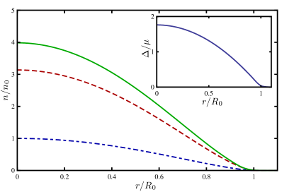
Figure 1: (Color online) The density profiles of the normal phase and the superfluid phase of a balanced unitary gas at zero temperature. Both calculated using the Bogoliubov-de Gennes method. Besides a small smoothening near the edge, this gives the same result as LDA. The dash-dotted line is the ideal-gas result, here $R_{0}$ is the radius of the ideal gas cloud and $n_{0}$ the central atomic density. The dashed line is the normal phase with self-energy effects and the solid line the superfluid phase. The inset shows the gap parameter for the superfluid phase.

The self-energy depends on the pseudospin of the particle and can be added to the Hamiltonian of Eq. (6) in the following way,

$$\bm{H}_{nl}^{\text{tot}}=\bm{H}_{nl}-\frac{2m}{\hbar^{2}}\begin{pmatrix}\hbar\Sigma_{+}(\bm{x})&0\\ 0&\hbar\Sigma_{-}(\bm{x})\\ \end{pmatrix}\;.$$ (20)

In the polarized case, these self-energies are really different from each other, and cannot be written in the same form as the chemical potential, such that the difference is a constant independent of position. This means that the $E^{\prime}\rightarrow-E^{\prime}$ symmetry of the Bogoliubov-de Gennes equation is gone. The BCS coherence functions $u_{\bm{n}}$ and $v_{\bm{n}}$ thus have to be computed independently for positive and negative energies. For the gap equation we can only use Eq. (11) and for the densities only Eq. (17).

The self-energy originates from the interaction, which is only nonzero for particles of different species. Therefore we take the majority(minority) self-energy proportional to the majority(minority) atomic density. From the Monte-Carlo results Lobo et al. (2006); Pilati and Giorgini (2008) the equation of state is known for a highly polarized mixture at unitarity. From this equation of state we can extract an accurate approximation to the self-energy. When we assume that all interaction effects are incorporated by the self-energies, the equation of state becomes

$$\frac{E}{V}=\frac{3}{5}\frac{\hbar^{2}}{2m}(6\pi^{2})^{2/3}(n_{+}^{5/3}+n_{-}^{5/3})+n_{+}n_{-}\Gamma\;,$$ (21)

where we already used that $\hbar\Sigma_{\sigma}=n_{-\sigma}\Gamma$. Symmetry arguments and dimensional analysis suggest the following form for the effective interaction,

$$\Gamma=-\frac{3}{5}\frac{\hbar^{2}}{2m}(6\pi^{2})^{2/3}\frac{A}{(n_{+}^{\alpha}+n_{-}^{\alpha})^{1/3{\alpha}}}\;,$$ (22)

with $\alpha$ a fit parameter and $A$ can in principle be obtained from a simple ladder calculation. This equation of state overlaps very accurately with the Monte-Carlo equation of state for $\alpha=3$ and $A=0.96$. The resulting self-energies can be directly added to the Bogoliubov-de Gennes equations. In the normal state and in the limit of large $\mu\gg\hbar\omega$, the results of the Bogoliubov-de Gennes equations are equal to the local density approximation, with the exception of boundary effects as shown in Fig. 1.

II.3 Superfluid phase

The self-energies we use for the normal phase are not correct for the superfluid phase. In order to improve on that we can add a superfluid correction. The simplest way to do that is to include a second-order correction in $\Delta$. From other workGubbels et al. (2006); Astrakharchik et al. (2004b); Carlson and Reddy (2005) it is known that the balanced unitary superfluid behaves like a BCS superconductor with a scaling factor of the chemical potential. In BCS theory, the relation between the chemical potential and the Fermi energy is $\mu=(1+\beta_{\text{BCS}})\epsilon_{\text{F}}$ with $\beta_{\text{BCS}}=-0.41$ and $\epsilon_{\text{F}}=\hbar^{2}(6\pi^{2}n)^{2/3}/2m$. For the unitarity Fermi gas this relation is $\mu=(1+\beta)\epsilon_{\text{F}}$ with $\beta=-0.59$. This scaling can be incorporated in the self-energy as $\mu^{\prime}=\mu-\hbar\Sigma$, where $\mu^{\prime}$ then plays the role of the chemical potential in BCS theory, from which it follows that $\mu^{\prime}=(1+\beta_{\text{BCS}})\epsilon_{\text{F}}$. We thus obtain that $\hbar\Sigma=(\beta-\beta_{\text{BCS}})\epsilon_{\text{F}}$. The self-energy we find using this scaling, can be compared with the equal density one from Eq. (22). It follows that both self-energies are equal for $A_{\text{sf}}=0.32$. The $\alpha$ is not fixed with the scaling approach and therefore we use $\alpha=3$. This smaller value of $A$ shows that the normal self-energy overestimates the diagonal self-energy in the superfluid phase.

In this paper we want to investigate what happens at the surface between the normal and the superfluid phase in the imbalanced trapped Fermi mixture. To do this we need the self-energy not only in the equilibrium normal and superfluid phase separately, but also out of equilibrium. We achieve this by considering a $|\Delta|^{2}$ correction to the self-energy. We thus write for the effective interaction,

$$\Gamma=-\frac{3}{5}\frac{\hbar^{2}}{2m}(6\pi^{2})^{2/3}\frac{A-(A-A_{\text{sf}})\frac{|\Delta|^{2}}{|\Delta_{0}|^{2}}}{(n_{+}^{3}+n_{-}^{3})^{1/9}}\;,$$ (23)

here $|\Delta_{0}|=1.67\mu$ is the value of the gap in the balanced superfluid for our modified BCS theory with self-energy effects. Within Bogoliubov-de Gennes theory this self-energy now incorporates the correct equation of state for both the normal and the superfluid phase. With this we can thus study the behavior around the interface.

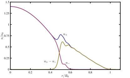
Figure 2: (Color online) The density profiles of the polarized superfluid in the unitarity limit at zero temperature calculated using the Bogoliubov-de Gennes method. The interface between the normal and superfluid phase is clearly visible, and has a nonzero width. The minority density, however, drops quickly to zero after the interface, which is in contrast with experiments. We used $\mu=21\hbar\omega$ and about $P=0.48$ for the polarization. The scaling is as in Fig. 1, with $R_{0}$ and $n_{0}$ for the majority species.

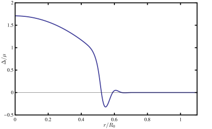
Figure 3: (Color online) The gap parameter for a polarized superfluid in the unitarity limit calculated using the Bogoliubov-de Gennes method. The interface between the normal and superfluid phase is clearly visible, and has a nonzero width. Near the interface, oscillations are clearly visible. The physical parameters are the same as in Fig. 2.

An interface appears when we consider a population imbalance in the Fermi mixture. We can arrive at this by setting the chemical potential difference $h$ to a nonzero value. In principle the Bogoliubov-de Gennes method solves such a system, however, in practice there are technical details that decrease the efficiency of the iterative process used to find a solution to the gap equation. The major difficulty is that different energy levels can get close together, such that they are not easily distinguished. In order to find all energy levels up to the cutoff, a very good guess of the energy is needed to start with. To get a good guess, we start with the gap and self-energy set to zero, so that the energies are given by Eq. (7), and slowly increase them. This method, although time consuming, works very well. However, this in turn gives rise to avoided crossings that complicates the algorithm to guess the energies. The resulting algorithm is rather slow, but fast enough to give results after a few hours of computer running time.

II.4 Results

The approach using the Bogoliubov-de Gennes equations together with the gap equation, works well in the sense that it converges to a reasonable function for the gap. Most of the results plotted in this paper are performed with the chemical potential $\mu=21\hbar\omega$. This value is chosen for numerical convenience, since it is large enough that most finite-size effects are small, but not too large such that a result can be found within a reasonable amount of time. This value of the chemical potential corresponds to about $2\times 10^{4}$ particles, which is somewhat less than used in experiments that have about $10^{5}$-$10^{7}$. The dependence on the total number of atoms can, however, be scaled away in the unitarity limit, as is done in the figures as well as with the data of MIT. Only finite-size effects near the edge or the interface are affected by the total number of atoms.

In Fig. 5 the $u$’s and $v$’s for some one-particle eigenstates are plotted. This shows that the states near the Fermi surface deviate substantially from the harmonic oscillator states, whereas for larger energies they become more alike. The fact that the harmonic oscillator states are a good approximation for large energies is used when dealing with the regularization of the divergence in the gap equation Eq. (14). In Fig. 4 the energy spectrum for $l=0$ is shown for both the polarized and the balanced superfluid. The polarized energies are clearly not symmetric for $E^{\prime}_{n}\rightarrow\ -E^{\prime}_{-n}$ whereas the balanced energies have this symmetry. Notice that in both cases, the chemical potential difference $h$ is absorbed in the energies. The difference between the positive en negative branch is thus entirely caused by the difference in the self-energies.

The Bogoliubov-de Gennes equations with the gap equation and the self-energy effects included, seems to describe the observed physics rather well. However, a closer look shows problems with this method. These problems are critical when looking at the interface in the Fermi mixture. The two most important problems are the oscillations that appear near the interface and the incorrect location of the interface itself.

The location of the interface is determined by the gap equation, which in normal BCS theory minimizes the thermodynamic potential. However, in the polarized case, the phase transition is a first-order transition. This means that the thermodynamic potential close to the phase transition has two minima and a maximum, all of which are a solution to the gap equation. The real transition should occur when the value of the thermodynamic potential in the $\Delta=0$ minimum becomes lower than its value in the other superfluid minimum. This condition crucially depends on the actual value of the thermodynamic potential in the superfluid minimum. Although this value is known from other analysis, see Eq. (26) below, it is not included in this model. Because of this problem, the interface is shifted outwards and as a result almost completely removes the partially-polarized shell from the theory.

The oscillations in the gap parameter and the density profiles are related to the proximity effect near the interfaceMcMillan (1968). This seems to be a common feature in many Bogoliubov-de Gennes analysis Kinnunen et al. (2006); Tezuka and Ueda (2008); Liu et al. (2007); Machida et al. (2006) and also appears in balanced BCS theory when studying a normal-superfluid interface. We believe this is not a signature of an FFLO phase in the gas, because for that the homogeneous phase diagram should contain a so-called Lifshitz point where the superfluid density becomes negative and it is energetically favorable to form Cooper pairs with a nonzero center-of-mass momentum. But we have checked that this theory at unitarity does not contain such a Lifshitz point Gubbels et al. (2009). The oscillations are also not related to the self-energy contributions, however, the oscillations are enhanced by it as the self-energies depend on the gap parameter. In the current theory, no extra costs for gradients in the gap parameter are included, which would clearly suppress these oscillations.

The problems with the Bogoliubov-de Gennes approach are difficult, if not impossible to overcome within this framework. We therefore believe that a different approach, using Landau-Ginzburg theory, in which a gradient effects for the gap parameter can be easily taken into account, works much better. The position of the interface can then correctly be included by choosing the correct self-energies. The oscillations will be suppressed as a result of gradients contributions that introduces an extra energy cost for rapid variations in the gap. How this works in practice is discussed next.

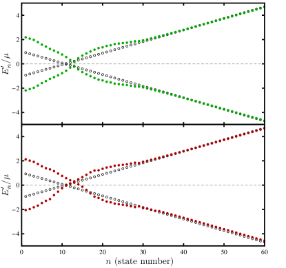
Figure 4: (Color online) The energy spectrum in the unitarity limit for zero angular momentum $l=0$ for the normal state (open dots), the balanced superfluid (upper figure) and the polarized superfluid (lower figure).

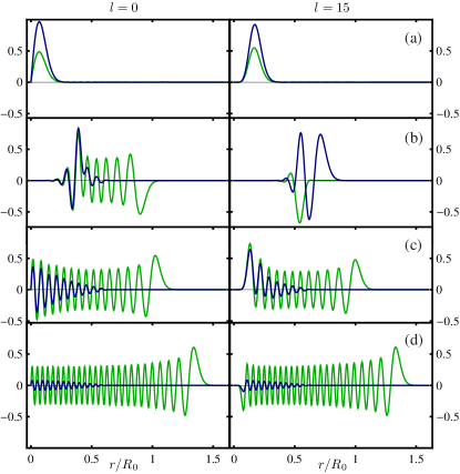
Figure 5: (Color online) Some examples of eigenstates of the trapped Fermi mixture. The two lines are the $u_{nl}(r)$ (light green line) and $v_{nl}(r)$ (dark blue line) functions from the Bogoliubov transformation in Eq. (4). In the left column states with angular momentum zero $l=0$, and in the right column with $l=15$. On the rows (a) through (d), states with increasing $n$ are shown. The state in (b) is near the Fermi-surface and thus deviates most from the harmonic oscillator states, while in (d) the $n$ is very large and the states look more like the harmonic oscillator states.

III Landau-Ginzburg

In the previous section we discussed the Bogoliubov-de Gennes method to study beyond local-density behavior in the vicinity of the superfluid-normal interface. We want to stress once more that this method experiences problems in a system with a first-order transition, that can not be readily resolved. Therefore, to obtain a more detailed picture of the interface we need a different approach. Because we want to describe a first-order phase transition, the location of the transition, and therefore the interface, is determined by the values of the thermodynamic potential in its minima. To do this correctly we need an appropriate thermodynamic potential that describes both the normal and the superfluid phase. This thermodynamic potential can then be extended with a gradient term to take the energy cost of a varying gap parameter into account.

We arrive at our most accurate theory for the inhomogeneous Fermi mixture in the unitarity limit by constructing an approximation to the exact Landau-Ginzburg (grand-canonical) energy functional $\Omega[\Delta(x);\mu,h]$ for the BCS gap parameter $\Delta(x)$. Here, $\mu_{+}=\mu+h$ and $\mu_{-}=\mu-h$ are again the chemical potentials for the majority and minority atoms respectively. The approach is very different from the previous approach based on the Bogoliubov-de Gennes equations. Although these equations exactly diagonalize the fermionic part of the microscopic action, the BCS gap parameter is then only obtained in the saddle-point approximation. As a result, crucial fluctuation corrections are missing in the strongly interacting limit. While self-energy corrections can still be readily included in the Bogoliubov-de Gennes approach, diagrammatic vertex corrections to the particle-particle correlation function that also affect the gap equation are neglected.

III.1 Normal phase

The Landau-Ginzburg approach is based on the central idea that the relevant physics of the strongly interacting system is not only captured by fermionic self-energy insertions, but that also gradients of the order parameter are important. In this context it is important to realize that there exists an exact energy functional $\Omega[\Delta;\mu,h]$ that describes the system exactly and that we thus want to approximate as best as we can. As a first step towards this goal we can use mean-field theory, because it is now rather well established that mean-field theory gives a correct qualitative description of the unitarity limit. Namely, at zero temperature both experiments and several Monte Carlo calculations find a first-order transition at a local critical imbalance of about $P_{c}=0.4$, while for the balanced case both find a second-order phase transition at about $T_{c}=0.15T_{F}$. The second and first-order transitions should then be connected by a tricritical point as confirmed experimentally. Since the BCS energy functional gives rise to the same qualitative behavior it must have the same shape and temperature dependence as the exact functional. We therefore start with BCS theory, after which we include the dominant effects we are still missing. The BCS energy functional is

$$\Omega_{\text{BCS}}[\Delta;\mu,h]= \sum_{\bm{k}}\left(\epsilon_{\bm{k}}-\mu-\hbar\omega_{\bm{k}}+\frac{|\Delta|^{2}}{2\epsilon_{\bm{k}}}\right)$$ (24)

$$-k_{\text{B}}T\sum_{\bm{k},\sigma}\log\left(1+\text{e}^{-\hbar\omega_{\bm{k},\sigma}/k_{\text{B}}T}\right)~{},$$

where $\epsilon_{\bm{k}}=\hbar^{2}\bm{k}^{2}/2m$, $m$ is the mass, and the superfluid dispersion is $\hbar\omega_{\bm{k}}=\sqrt{(\epsilon_{\bm{k}}-\mu)^{2}+|\Delta|^{2}}$. The second sum is over the pseudo-spin $\sigma=\pm$ with $\hbar\omega_{\bm{k},\sigma}=\hbar\omega_{\bm{k}}-\sigma h$.

Since BCS theory incorrectly leads to a noninteracting normal state, we first incorporate the fermionic self-energy effects, such that we are able to correctly describe the strongly interacting normal state. To incorporate self-energy effects, we have to replace the chemical potentials by their renormalized versions $\mu_{\sigma}^{\prime}=\mu_{\sigma}-\hbar\Sigma_{\sigma}$, where $\hbar\Sigma_{\sigma}$ are the appropriate fermionic self-energies. Inspired by Hartree-Fock theory we take in the normal state the following Ansatz Gubbels et al. (2006)

$$\mu_{\sigma}^{\prime}=\mu_{\sigma}+\frac{3}{5}A\frac{(\mu_{-\sigma}^{\prime})^{2}}{\mu_{+}^{\prime}+\mu_{-}^{\prime}}\;.$$ (25)

From the Monte Carlo result for a fully polarized gas Lobo et al. (2006), we know that minority particles start to appear at zero temperature when $\mu_{-}=-0.6\mu_{+}$. This fixes the prefactor in the Ansatz for the self-energy which is then the same as in Eq. (22). This construction leads to excellent agreement with the full Monte Carlo equation of state. This is very nicely illustrated in Fig 2. of Ref. Gubbels et al. (2009) (dashed line) were the same self-energy is used. As a result, we are thermodynamically completely equivalent to Monte Carlo calculations in the normal state at zero temperature. Moreover, we have also checked that our construction leads to the correct Monte Carlo result for the balanced gas at $T_{c}=0.15T_{\text{F}}$. Namely, our construction also gives $\mu=0.5\epsilon_{\text{F}}$ just as found in Ref. Burovski et al. (2006). This agrees with our assumption that the coefficient $A$ does not depend too much on temperature in the normal state.

This form of the self-energy is closely related to the one in Eq. (22), which can be seen by replacing the densities with the ideal gas value. These two different forms behave similar for the normal phase, but for the superfluid phase it is clear that the self-energy in Eq. (25) has not the correct behavior. To account for this we will introduce the necessary corrections in the next subsection.

III.2 Superfluid phase

We now turn to the superfluid state. Since at zero temperature a phase separation occurs between the normal state and a balanced superfluid, the (diagonal) self-energy in the balanced superfluid is also important for our purposes. Since both our normal state construction and the use of BCS theory take interaction effects into account in the superfluid state, there are double counting problems. To correct for this, the strategy is again too match the superfluid Monte Carlo result, so that the coefficient of our extra superfluid self-energy correction is uniquely fixed by the known value for the energy in the superfluid minimum. In the superfluid phase it is much harder to calculate self-energy corrections from first principles, however, what can be shown analytically is that corrections to the self-energy in the superfluid state can be expanded as a series with even powers in the gap parameter. As a result, the direct way to account for the superfluid self-energy effects is by matching a second-order correction in the BCS gap parameter Bulgac and Forbes (2008) to Monte Carlo. This can be accomplished by adding $\varDelta\Sigma_{\sigma}=0.21\Delta^{2}/\hbar\mu^{\prime}$ to the self-energies. The proportionality constant is fixed by the requirement that in the balanced case the minimum of the energy functional equals

$$\Omega_{\text{cr}}/V=-\frac{4\sqrt{2}\mu^{5/2}m^{3/2}}{15\pi^{2}\hbar^{3}(1+\beta)^{3/2}}\;,$$ (26)

with $\beta=-0.58$ and $V$ the volume. Also, the critical imbalance for phase separation is now automatically incorporated exactly into the theory at zero temperature.

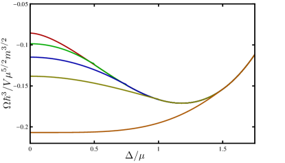
Figure 6: (Color online) The zero temperature energy functional as a function of the order parameter $\Delta$ with the self-energy of Eq. (23) for different values of $h$.

At this point our construction gives rise to one last problem, namely that the terms in the thermodynamic potential that describe the condensate of Cooper pairs, still depends on $h$ in the superfluid state through the renormalization $\mu^{\prime}(\mu,h)$. This is not correct, because at zero temperature the phase separation occurs between a partially polarized normal state and an unpolarized superfluid. To solve this problem, we have chosen to exponentially suppress the $h$ dependence in the superfluid state, which then finally leads to the correct shape of the thermodynamic potential in all known limits. Technically this is achieved by writing $\mu^{\prime}$ in terms of $\mu$ and $h$ while exponentially suppressing the $h$ dependence through the substitution $h\rightarrow h\exp{(-4|\Delta|^{2}/\mu^{2})}$. The factor of 4 in the exponent of the suppression is somewhat arbitrary, but it is large enough to make the $h$ dependence in the ground state superfluid minimum vanish. Slight variations in this factor do not affect our results. Note that the whole problem is truly artificial, since if we would have calculated the self-energy corrections in terms of the densities rather than the chemical potentials, then all $h$-dependence would have been automatically exponentially suppressed in the superfluid state. This is what was done in the previous part using Eq. (23) and is shown explicitly in Fig. 6, where the energy-functional is plotted for the density dependent self-energy in Eq. (22). The energy-functional we just constructed with the self-energy given above Eq. (25) is shown in Fig. 7 and has the same behavior as a function of $h$ as in Fig. 6. This thus proves that this suppression of the $h$ dependance captures the correct and relevant physics. The reason that the energy functional with the self-energy of Eq. (25) is preferred, is that it does not directly depend on the densities. This makes it consistent with the use of the grand-canonical ensemble and much easier to use.

Now our theory gives the correct equation of state in both the superfluid and the normal phase and thus also the correct critical polarization. Even the outcome for the universal number $\zeta=\Delta/\mu$ of the balanced superfluid ground state is reasonable. Here, we find $0.97$ while Monte Carlo gives $1.07\pm 0.15$ Carlson and Reddy (2008, 2005). Moreover, our functional also provides a theoretical description of the system in case the order parameter is not in a minimum of the thermodynamic potential as illustrated in Fig. 7. This is very important for our purposes as it can be used to study also the superfluid-normal interface.

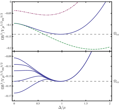
Figure 7: (Color online) The zero temperature energy functional as a function of the order parameter $\Delta$. The upper panel illustrates the balanced case, where the dash-dotted line is the usual BCS result, the dashed line incorporates only the normal state self-energy effects, and the solid line includes also the superfluid $\varDelta\Sigma_{\sigma}$ correction. In the lower panel the energy functional is shown for various values of the chemical potential difference $h$, with $h_{\text{cr}}=0.94\mu$ its critical value.

To go beyond LDA, we now take into account the gradient term in the energy functional, resulting in

$$\begin{split}\Omega[\Delta;\mu,h]=&\Omega_{\text{BCS}}[\Delta;\mu^{\prime},h^{\prime}]\\ &+\frac{1}{2}\int\operatorname{d}\!\bm{x}~{}\gamma(\mu,h)|\nabla\Delta|^{2}\;,\end{split}$$ (27)

where $\hbar\gamma(\mu,h)\sqrt{\mu/m}$ is a positive function of the ratio $h/\mu$ only. This changes the discontinuous step at the interface obtained within LDA, into a smooth transition. A careful inspection of the interface in the data of Shin et al. Shin et al. (2008), cf. Fig. 8, also reveals that the interface is not a sharp step. This is most clear in the data of the density difference, since the noise in the difference is much smaller than in the total density. This has to do with the experimental procedure used, which independently measures the total density and density difference. As we have seen, a smooth transition arises also in the self-consistent Bogoliubov-de Gennes equations. But these lead then also to oscillations in the order parameter and the densities, due to the proximity effect McMillan (1968). This is not observed experimentally. Oscillations will also occur in our Landau-Ginzburg approach if $\gamma(\mu,h)<0$. However, we have checked both with the above theory as well as with renormalization group calculations Gubbels and Stoof (2008) that $\gamma(\mu,h)$ is positive. This agrees with the phase diagram of the imbalanced Fermi mixture containing a tricritical point and not a Lifshitz point in the unitarity limit Gubbels et al. (2009).

We restrict ourselves here to a gradient term that is of second order in $\Delta$ and also of second order in the gradients. There are of course higher-order gradient terms that may contribute quantitatively Stoof (1993), but the leading order physics is captured in this way due to the absence of a Lifshitz transition. One way to compute the coefficient $\gamma(\mu,h)$ is to use the fact that in equilibrium this coefficient can be exactly related to the superfluid stiffness, and therefore the superfluid density $\rho_{\text{s}}$, by $\gamma=\hbar^{2}\rho_{\text{s}}/4m^{2}|\langle\Delta\rangle|^{2}$. At zero temperature it gives the simple result that $\gamma(\mu,h)=\sqrt{m/2\mu}/6\pi^{2}\hbar\zeta^{2}(1+\beta)^{3/2}$, with $\beta$ and $\zeta$ universal constants as defined earlier.

IV Comparison with Experiments

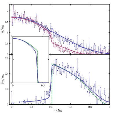
Figure 8: (Color online) The density profiles of a unitary mixture with polarization P=0.44 in a harmonic trap. The upper figure shows the majority and minority densities as a function of the position in the trap. The lower figure shows the density difference, where the theoretical curves show the results both within LDA (dashed line) and for our theory (solid line) that goes beyond this approximation and, therefore, allows for a substantial better agreement with experiment. The inset shows the BCS gap parameter $\Delta(r)$ both for LDA (dashed line) and our theory (solid line). The experimental data (dots) and scaling is from Shin et al. Shin et al. (2008).

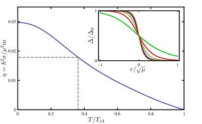
Figure 9: (Color online) The surface tension as a function of the temperature, computed in the homogeneous case at unitarity. The temperature is scaled by the temperature of the tricritical point. The dashed line shows the value used to compare with experiments. The inset shows the gap around the interface for several temperatures ($0.9$, $0.7$, $0.5$, $0.25$ and $0.01$ $T_{\text{c}3}$).

Up to now we have focussed on the zero temperature limit. However, our arguments are also valid for nonzero temperatures $T\ll T_{F+}$, with $T_{\text{F+}}$ the Fermi temperature of the majority species. Here we are allowed to neglect the temperature dependence of the self-energies and the superfluid density. The data of Shin et al. of interest to us is taken at a temperature of $0.03T_{\text{F+}}$. This is about a third of the temperature at the tricritical point $T_{\text{c3}}$. A nonzero temperature significantly affects the surface tension and increases the width of the interface, because it lowers the energy barrier between the normal and superfluid phases. Indeed at the tricritical point this barrier, and thus the surface tension, exactly vanishes. We therefore also perform calculations at $0.3T_{\text{c3}}$. As mentioned, the leading-order temperature effects are incorporated in the BCS energy functional of Eq. (24).

IV.1 Surface Tension

The fact that we are able to study the superfluid normal interface beyond LDA, makes it possible for us to also determine the surface tension. The surface tension is given by the (grand-canonical) energy difference between a one-dimensional LDA result with a discontinuous step in $\Delta(z)$ and our Landau-Ginzburg theory with a smooth profile for the order parameter $\Delta(z)$. To write the surface tension $\sigma$ in a dimensionless form, we use $\sigma=\eta(m/\hbar^{2})\mu^{2}$, with $\eta$ a dimensionless number. In this form it was previously found that for the Rice experiment $\eta=0.6$ Partridge et al. (2006a). This was extracted from the large deformations of the superfluid core observed in that experiment. The experiment of Shin et al. Shin et al. (2008) does not show any deformation, which puts an upper bound on $\eta$ of about $0.1$ Haque and Stoof (2007); Baur et al. (2009).

The size of the interface is rather small compared to the size of the whole trap. This makes it possible to compute the surface tension of the interface in a homogeneous system rather than in the whole trap. In Fig. 9 the surface tension of this model is plotted as a function of the temperature. At the tricritical point the surface tension vanishes and at zero temperature it is about $\eta=0.03$. For a more realistic temperature of about $0.3T_{\text{c3}}$ we find $\eta=0.02$ which is significantly smaller than the critical surface tension that would cause deformation. This is thus in agreement with the MIT experiment.

We now give a more detailed discussion of our analysis of the density profiles observed by Shin et al. In experiments the cloud is trapped in an anisotropic harmonic potential, which is in the axial direction less steep than in the radial direction. However, since the gas cloud shows no deformations in this case we can in a good approximation take the trap to be spherically symmetric. The order parameter then depends only on the radius and the total Landau-Ginzburg energy is given by integrating the Landau-Ginzburg energy density over the trap volume. To account for the trap potential in the energy functional we let the chemical potential depend on the radius, such that we have $\mu_{\sigma}(r)=\mu_{\sigma}-V(r)$, with $V(r)$ the effectively isotropic harmonic potential.

To find the order parameter as a function of the radius we have to minimize the energy functional with respect to the order parameter, thus $\delta\Omega[\Delta;\mu,h]/\delta\Delta(r)=0$. This gives a second-order differential equation for $\Delta(r)$. Solving this Euler-Lagrange equation, with the proper boundary conditions in the center of the trap, gives a profile for $\Delta$ as is shown in the inset of Fig. 8. This profile of the order parameter is much smoother than the discontinuous step one obtains within LDA that is also shown in Fig. 8. Besides this, there are two more aspects that deserve some attention. First, we notice that the value of the gap at the original LDA interface is decreased by almost a factor of three and, second, the gap penetrates into the area originally seen as the normal phase. This behavior makes the gap for a small region smaller than $h^{\prime}$, giving locally rise to a gapless superfluid, which implies a stabilization of the Sarma phase.

Before discussing this particular physics, we focus first on the density difference. To obtain the density profiles within our theory, the thermodynamic relation $n_{\sigma}(r)=\partial\Omega/\partial\mu_{\sigma}(r)$ is used, where $n_{\sigma}$ is the density of particles in state $\sigma$ and $\mu_{\sigma}(r)$ the associated local chemical potential. It is important that, because of the self-energy effects, we cannot use the standard BCS formulas for the density, but really have to differentiate the energy functional. In BCS theory this would of course be equivalent. Given the density profiles, the comparison between theory and experiment can be made and is ultimately shown in Fig. 8. Overall the agreement is very good. Theoretically the interface appears to be somewhat sharper than observed. This can be due to higher-order gradient terms, that are neglected in the calculation and that would give an additional energy penalty for a spatial variation of the order parameter. There are however experimental effects that could make the interface appear broader, for instance, the spatial resolution of the tomographic reconstruction or the accuracy of the elliptical averaging Ketterle and Shin .

The Landau-Ginzburg approach presented here, shows some new features compared to LDA. One interesting feature is the kink, that is clearly visible in the majority density profile shown in Fig. 8. Notice that this kink appears before the original (LDA) phase transition from the superfluid to the normal phase. This kink signals a crossover to a new exotic phase, namely the gapless Sarma phase. Note that at zero temperature it becomes a true quantum phase transition. At the crossover, the order parameter becomes smaller than the renormalized chemical potential difference $h^{\prime}$ and the unitarity limited attraction is no longer able to fully overcome the frustration induced by the imbalance. As a result the gas becomes a polarized superfluid. Because the gap $\Delta$ is smaller than $h^{\prime}$ this corresponds to a gapless superconductor. In a homogeneous situation this can, far below the tricritical temperature, never be a stable state. However, because of the inhomogeneity induced by the confinement of the gas, the gap is at the interface forced to move away from the local minimum of the energy functional and ultimately becomes smaller than $h^{\prime}$. The Sarma state is now locally stabilized even at these low temperatures. Notice that this is a feature of a smooth behavior of the gap and that the presence of the Sarma phase does not depend on the quantitative details of the energy functional $\Omega[\Delta;\mu,h]$.

V Conclusions

In this paper we first studied the Bogoliubov-de Gennes method to go beyond LDA. We showed that the addition of a self-energy gives a model that reproduces the known Monte-Carlo results of the homogeneous system. However, we argued that this Bogoliubov-de Gennes approach suffers from some fundamental difficulties and that an approach using Landau-Ginzburg theory gives more accurate results. We used results from Monte-Carlo calculations to construct an approximation to the exact Landau-Ginzburg energy functional that describes the experimental data without any free parameters. We considered beyond LDA effects on imbalanced Fermi mixtures in the unitarity limit and showed that this results in a much better agreement with experiments than LDA. The interface details will depend on both the polarization and temperature, but there is not sufficient experimental data available for such a systematic study. Moreover, we found that exotic physics is occurring in the superfluid-normal interface. We also showed that an experimental signature of the gapless Sarma phase is a kink in the majority density profile. The temperature plays an important role here, since a lower temperature will lead to a more visible kink but also to a sharper interface. Presumably a compromise will have to be found in this respect. We hope that our work will stimulate more experimental work in this direction.