Gravitational Microlensing: A parallel, large-data implementation¹

Abstract

Gravitational lensing allows us to probe the structure of matter on a broad range of astronomical scales, and as light from a distant source traverses an intervening galaxy, compact matter such as planets, stars, and black holes act as individual lenses. The magnification from such microlensing results in rapid brightness fluctuations which reveal not only the properties of the lensing masses, but also the surface brightness distribution in the source. However, while the combination of deflections due to individual stars is linear, the resulting magnifications are highly non-linear, leading to significant computational challenges which currently limit the range of problems which can be tackled. This paper presents a new and novel implementation of a numerical approach to gravitational microlensing, increasing the scale of the problems that can be tackled by more than two orders of magnitude, opening up a new regime of astrophysically interesting problems.

1 Introduction

Since the identification of the first multiply-imaged quasar (Walsh et al., 1979), gravitational lensing has been used to probe the distribution of matter on many astrophysical scales, such as planets (Gaudi et al., 2008), individual galaxies (e.g. Brewer & Lewis, 2008; Dye et al., 2008), clusters (e.g. Deb et al., 2008; Sand et al., 2008), and large-scale structure (e.g. Kitching et al., 2008; Wang et al., 2009). Soon after the discovery of the first gravitational lens, it was realised that individual stars within a lensing galaxy would themselves act as lenses (Chang & Refsdal, 1979), and while the separation of the resulting images would be too small to be resolved, this microlensing can significantly magnify the background source. Furthermore, given the density of compact objects within galaxies (such as stars and possible dark matter), it was clear that many objects will influence the path of a beam of light as it traverses a galaxy, and beyond considering only a couple of lensing masses, the study of microlensing becomes analytically intractable and must be tackled numerically (Young, 1981; Paczynski, 1986).

The first observations of microlensing were made in 1989 (Corrigan et al., 1990; Irwin et al., 1989), in 2237+0305, a distant quasar (z = 1.695) lensed into four images by a nearby spiral galaxy (Huchra et al., 1985); it has been photometrically monitored for two decades (Udalski et al., 2006), revealing exquisite light curves for each of the images, clearly revealing the presence of gravitational microlensing. Furthermore, the number of potentially microlensed quasars has steadily increased (Eigenbrod et al., 2006; Gunn et al., 1979; Myers et al., 1999; Reimers et al., 2002; Turner et al., 1989; Vanderriest et al., 1983) and hence an efficient means of theoretically understanding gravitational microlensing is required.

2 Microlensing Ray-Tracing

2.1 Mathematical Framework

This paper does not intend to derive the basic gravitational lensing equations, the reader is directed towards the excellent textbook by Schneider et al. (1992) and thesis by Wambsganss (1990). For microlensing calculations a normalized lens equation in the following form is used to map the ray from the observer, through the lens, and into the source:

$$\vec{y}=\left(\begin{array}[]{ccc}1-\gamma&0\\ 0&1+\gamma\end{array}\right)\vec{x}-{\sigma}_{c}\vec{x}-\sum_{i=1}^{N_{*}}\frac{m_{i}(\vec{x}-\vec{x_{i}})}{(\vec{x}-\vec{x_{i}})\textsuperscript{2}}.$$ (1)

Here, $\vec{x}$ and $\vec{y}$ are the location of a light ray in the lens and source plane respectively, $\vec{x_{i}}$ and $m_{i}$ are the mass and co-ordinates of the ith microlensing star. For the remaining terms in this expression, $\sigma_{c}$ represents the local density of smooth matter in the galaxy, whereas $\gamma$, known as the shear, encapsulates the large scale asymmetry in the galaxy mass distribution. The surface density of compact objects (assumed to be uniform), is also used in modelling and simulations and is given by $\sigma_{s}$. The distance scale used in lensing is the Einstein Radius (ER), the radius of a ring produced by lensing of a source that is directly behind a point lens in a line from lens to observer. Einstein Radii are used to refer to the extent of observed images on the sky, and are derived from the mass of the lens and the distances to the lens and source.

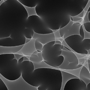
Figure 1: An example of a gravitational microlensing magnification map generated via inverse ray tracing. The lens consists of 435 stars each of 1 solar mass (M_⊙), randomly distributed, with mass parameters $\sigma_{s}$ = 0.39, $\gamma$ = 0.10. The viewing window is 8 ER in width. Light shading corresponds to regions of high magnification, whereas darker regions represent demagnification.

2.2 Numerical Approach

Clearly, Eqn 1 represents a mapping from a source location, $\vec{y}$, to a number of image (or observed) positions $\vec{x}$. However, it is apparent that this mapping is one-to-many, with a single source resulting in a number of images (dependent upon the number of microlensing masses $N_{*}$). However, reversing the mapping from the image plane back to the source is one-to-one and hence an “inverse ray-tracing” mechanism (Glassner, 1989) is typically employed in the study of microlensing. With this, the observer sends out a large number of rays into the image plane. For each ray, the deflection angle is calculated through Eqn 1 and the ray is mapped into the source plane and collected on a grid. After all the rays are followed, the density of rays in the binned-up map of their source positions is directly proportional to the magnification of a source at that location; Fig 1 presents an example of such a map, where light regions correspond to a high density of collected rays (i.e. strong magnification) whereas dark regions correspond to the opposite situation.

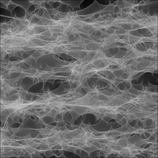
(a) 100% = 1 M_⊙, number of stars = 30496

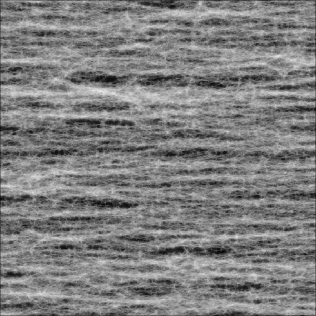
(b) 98% = 0.01 M_⊙, number of stars = 2989306

(c) 98% = 0.001 M_⊙, number of stars = 29887581

(d) 98% = Smooth, number of stars = 609

Figure 2: Magnification maps from simulations of bi-modal mass distributions. A total mass of 30496 $M_{\odot}$ is distributed in a circular lens plane of diameter 500 ER, with a viewing window of 20 $\times$ 20 ER. All simulations use $\gamma$ = 0.4250, with (a), (b) and (c) having $\sigma_{s}$ = 0.4750, $\sigma_{c}$ = 0 and (d) having $\sigma_{s}$ = 0.0095, $\sigma_{c}$ = 0.4655, so the total mass is the same in all. The first simulation (a) is a single-mass distribution of stellar masses, then in (b) and (c) some of the stellar mass is replaced with smaller compact objects, then in (d) that mass is replaced with smooth matter.

A deeper examination of Eqn 1 reveals that the computationally intensive aspect of undertaking such ray tracing is the sum over the microlensing masses when calculating the deflection angles; in typical simulations, there could be $10^{5}\rightarrow 10^{6}$ masses, with the tracing of $\sim 10^{11}$rays required to achieve sufficient density in the source plane. Following the seminal work by (Kayser et al., 1986), Wambsganss (1999) implemented an inverse ray-tracing approach which has become the “industry standard”, utilizing a tree-algorithm to ease the sum over the microlensing deflection angles. The advent of this approach has allowed the analysis of the magnification patterns of microlensed quasars (Wambsganss, 1992), the structure of quasar broad line emission regions (Keeton et al., 2006; Lewis & Ibata, 2004), chromatic effects in microlensing (Wambsganss & Paczynski, 1991), the nature of dark matter in lensing galaxies (Lewis & Gil-Merino, 2006; Pooley et al., 2008; Schechter & Wambsganss, 2002), and the effect of source size on microlensing (Bate et al., 2008; Mortonson et al., 2005), among others.

3 New Physical Challenges

Several quasar systems appear to possess anomalous flux ratios (Blackburne et al., 2006; Eigenbrod et al., 2006; Ota et al., 2006; Pooley et al., 2006), meaning that the observed image brightnesses differ significantly from predictions drawn from gravitational lens models possessing mass distributions that are smooth on galactic scales. Two key hypotheses have been put forward to explain these observations; either these anomalous ratios are due to millilensing by $\sim 10^{6}{\rm M_{\odot}}$ clumps of dark matter in the halo of the lensing galaxy (Chiba, 2002; Dalal & Kochanek, 2002; Metcalf, 2001; Mao & Schneider, 1998), or the quasars are microlensed by stars embedded in an overall smooth dark matter distribution (Witt et al., 1995). The former proposal is attractive as it may provide the first direct measurement of the missing substructure expected from galactic build-up in cold dark matter formation scenarios. The latter proposal is also important, potentially probing the fundamental nature of dark matter, as will be explained below.

The original proposal by Witt et al. (1995) considered a smooth dark matter component which actually suppresses the image flux for long periods, leading to the apparently anomalous flux ratios. However, Schechter & Wambsganss (2002) questioned this hypothesis, suggesting that the dark matter could in fact be composed of substellar compact objects, and that the existence of such a compact component could imprint itself on the resulting gravitational lens statistics. In studying the microlensing hypothesis, a number of of numerical simulations were undertaken by Schechter & Wambsganss (2002) using the backwards ray shooting approach, and Figure 2 illustrates several examples of the parameters employed. Figure 2(a) simulates a galaxy of a few thousand stars all of one solar mass (M_⊙), with $\sigma_{s}$ = 0.475 and $\gamma$ = 0.425. Figures 2(b) and (c) use the same parameters but two different masses for $\sigma_{s}$: 2% of the mass is in stars of mass M_⊙, and the rest is contained in small compact objects, 0.01M_⊙ in (b) and 0.001M_⊙ objects in (c). The final panel, Figure 2(d), presents the case of a smooth dark matter component ($\sigma_{s}$ = 0.0095, $\sigma_{c}$ = 0.4655, $\gamma$ = 0.425); as shown in (Lewis & Gil-Merino, 2006), when the mass of the compact dark matter component is made smaller, the general scale of caustic structure is reduced, although large scale caustic features, due to the presence of the solar mass stars in the simulations, remain. In comparing the lower two panels in Figure 2, the large scale caustic structure is the same in the small compact and smooth dark matter cases, but the smaller scale structure is quite different (in fact, it is non-existent in the smooth matter case). Lewis & Gil-Merino (2006) went on to show that, even though the large scale caustic structure is similar, the presence of the small scale caustics imprints itself on the statistical properties of the microlensing, with the lower panels possessing quite different magnification probability distributions. However, convolving these maps with a finite source radius washes out the small scale caustic structure, and for large enough sources the convolved compact mass and smooth mass magnification maps become statistically indistinguishable. This implies that there is a source scale size below which any compact matter component would appear as compact, and above which it would appear smooth, and hence observations of such systems at differing wavelengths (corresponding to differing source sizes) would probe the fundamental properties of dark matter.

However, the simulations undertaken to date have been limited by the computational power and memory of available computers; anomalous flux quasars are those that typically have been strongly magnified, requiring ray shooting through a large area to be statistically meaningful. Furthermore, these limitations place constraints on the number of dark matter lenses that can be considered, effectively placing a limit on the mass scale that can be simulated - around 10⁷ objects of mass 0.001 M${\odot}$. Hence, it was decided that a supercomputer implementation of the ray-shooting approach was required to tackle these physically interesting regimes.

4 A Supercomputing Approach

The numerical ray-shooting approach employs several approximations that have little impact on the accuracy but allow a significant improvement in performance. An examination of Equation 1 reveals that a $r^{-1}$ calculation is required for each lensing mass, the total deflection requiring a sum over all of these individual masses; of course, the calculation of the distance, $r$, involves the square roots, significantly adding to the computational load. The ray-tracing approach as adopted by Wambsganss (1999) reduces this load by use of a multipole expansion of the gravitational interaction for lensing masses far from the passage of the ray through the field of masses. For this, a cell tree is constructed by subdividing the distribution of lensing masses, with a constant regular subdivision until each cell holds a maximum of a single lensing mass. An opening angle criteria is then applied to distinguish between employing nearby masses as individual lenses, whereas more distant lens masses are grouped and a multipole expansion of their distribution is used to approximate their gravitational influences.

The use of the cell-tree substantially improves simulation run-time but substantially increases the amount of data required to run a simulation. All data is held in computer memory, and consists of:

• A 2-D array for the pixel map.

• An array of “stars”, each element containing the mass and location of a star in the galaxy. We will use the term “stars” to refer to all objects constituting the lens.

• An array for the cell tree, each element containing information about a cell and its location within the tree.

A typical simulation on a desktop computer may contain a pixel array of 2000$\times$2000 pixels and of order a million stars. This corresponds to 15 Mb for the pixel array, 38 Mb for the stars array, and 89Mb for the cell tree. The rays have no data existence; the result of shooting a ray is a pixel hit which is added to that pixel’s hit count. In the following, we outline the basic operation of the standard microlensing approach and the changes required to employ it in a supercomputer environment, successfully handling the significant computational and storage requirements to push the application of microlensing into a new scientific regime (see Section 5).

The starting point is to understand the operation of the standard ray shooting approach of Wambsganss (1999); this is expressed in the following pseudo-code

// Setup phase

Generate the stars, using a random distribution of locations and masses, within certain parameters

Sort the stars by encoding indexes

Generate the cell tree from the stars

Sort the cell tree by encoding indexes

// Shooting phase

Loop

Shoot a ray
Increment the pixel hit array where necessary
Move to a new location in the lens plane

Until the whole lens plane has been covered

The sorting operations of the stars and cell tree are required because during the shooting of the rays, searches are performed to determine the break between the employment of individual masses and expanded cells that are to be used for a particular ray, with the configuration changing as we consider rays traversing differing locations in the field of stars.

As noted in Section 3, we wish to increase the number of stars under consideration. Immediately, this significantly impacts the undertaking of microlensing simulations by desktop computers (which are limited by virtual memory to $\sim 20$ million stars), increasing the storage required for the masses and locations, as well as the tree structure. Furthermore, we additionally require an increase of the number of rays fired; as can be seen in Figure 2, the inclusion of small masses induces small scale structure in the magnification map, and to fully resolve this it is essential to increase the number of pixels covering the source, and the number of rays traced, to ensure we are not limited by counting statistics in the final map. In moving to a supercomputer environment, the following changes are required:

• Adapt the algorithmic approach of Wambsganss (1999).

• Parallelize the approach so it can exploit current multiprocessor computers; ray tracing is inherently parallelizable, as the rays are usually independent of each other. There are typically billions of rays in a microlensing simulation, which can be distributed in some appropriate way across many processors and shot concurrently.

• Increase the number of stars that can be considered, into the billions. This is an increase of a hundred-fold, and it is unlikely the data can be held in RAM with any reasonable architecture. Other strategies will be required to store the massive amounts of data that will be used.

• Change to an object-oriented paradigm; the approach of Wambsganss (1999) was originally implemented in Fortran 77 with procedural code and global data. It was decided that the supercomputer implementation would employ C++ as some objects such as the stars and cells naturally lend themselves to implementation as C++ class objects. Re-implementing in C++ will provide a sound basis for future work.

As the reimplementation in C++ is a design and development process we will describe it only briefly here. Data elements, such as stars and cells, were identified and reimplemented as C++ class types. The Fortran lensing algorithms were rewritten in C++ and combined with the C++ classes, producing a working program. The arrays that store the stars and cells were replaced with a C++ module that implements arrays as disk files (described later), but with a similar interface. Then the implementation was parallelized by sharing out the generation of stars, and the ray-shooting, to different processors (this is described later).

The rest of the paper focuses on the strategies used to parallelize our approach and increase the size of lenses available for microlensing research.

4.0.1 Parallelizing the ray shooting

For the supercomputer implementation, the rays that are shot need to be distributed across the available processors. There are many ways of parallelizing ray-tracing (Amri, 2003; Lee et al., 1998; Verdu et al., 1996) but little experience with this in gravitational lensing simulations. It does not matter which ray is executed on which processor, or in what order, as they are completely independent. We consider only static assignment of rays to processors, as dynamic assignment for load-balancing purposes is much more complicated and static assignment should be tried first. Dynamic load balancing is a model where job tasks (in this case rays) are assigned to processors at run-time based on the load on each processor as the simulation proceeds - idle processors get the next jobs, much like a multiprocessor operating system running user programs. Much more time and effort is required to implement dynamic load balancing compared to static load balancing. Static load balancing means that when the program runs, some algorithm at startup determines which ray is assigned to which process, and that is fixed for the duration of the simulation.

Therefore we are looking for a mapping

$$Assign(Ray)\mapsto Processor$$ (2)

which maps rays to processors for that run. There is a value for Assign which is optimal for a particular simulation, but it is unknown, so some heuristic is required. Mapping an equal number of rays to each processor is sufficient if there are many more rays than processors and each ray takes the same time. The latter is probably not going to be the case since the stars in the lens may not be not distributed evenly, and rays close to a lot of mass will take longer to process. We have adopted an interlaced ray distribution model: take a 2-D element dA of the lens plane and distribute the rays in that element across all processors, and do the same for all other elements. This means that every processor simulates lensing over the entire lens plane, but only some rays at each point of the lens plane. We hope that this will even out the load without the need for load balancing.

To implement parallelization we could employ either a multithreading or multiprocess model. Multiprocessing means that several parallel processes are created by the computer operating system and they must access shared data outside the program, for example on disk. In multithreading there is only a single process with parallel threads of execution running inside it, and all global data in the program is automatically shared between threads. Multithreading is usually more efficient but also more error-prone in development, so for a first implementation we opted for multiprocessing.

In the setup phase the generation of the stars can be parallelized by distributing the load evenly across all processes. The generation of the cells from the stars is a sequential process based on sophisticated location and tree indexing which cannot be easily parallelized. The sorting steps could be parallelized but have not been; this will be discussed in the next section. The shooting phase can be distributed across all processors.

4.1 Increasing the data storage

Pushing into the regime of $\sim$billion stars in a lens requires a stars array and cell tree of order 200GB; the following are possible ways of storing this data:

1. On a 64-bit computer with 200Gb RAM it could be stored in memory as it previously has been.

2. If simulations are to be run on many computers at the same time, and the computers collectively have enough memory, distribute the data in the memory of those machines.

3. Put the data in files on a shared disk, not in RAM.

Option 1 is possible and requires no modification of the data storage, although clearly requires a particular computer architecture not available in typical (i.e. beowulf) clusters. Option 2 is possible if enough machines are used with enough RAM; then data could be spread amongst them and fetched across the network. Option 3 can be used anywhere there is sufficient disk space, even on desktop computers. In our new implementation all three options were combined, as huge amounts of disk space are now common (more than large RAM machines), the simulation data is placed on disk, but partially cached in memory so that all the available RAM is used.

The stars array and cell tree were each replaced with a binary file, but still accessed like arrays, so that any object at any part of the file could be requested with an index. Naturally this means that file I/O will dramatically slow down the simulation, although it is envisaged that caching strategies and parallelizing the ray-shooting may compensate for this. Since shared files are trivial on modern networks, multiple processes can read data from a single set of shared files. When starting a simulation, several processes can create the files and the others wait until they are ready, or, each process can generate its own version of the files, which is very wasteful of disk space but means some processes may be able to start earlier.

4.2 Sorting with files

The sorting of stars and cells is inherent in the algorithms in the set-up phase that code the stars and cells for indexing and searching; it cannot be avoided without significant redesign of the cell tree usage. In the original implementation where data is in RAM, a heap-sort algorithm is used (Knuth, 1998). A heap sort swaps elements from the end of an array to the beginning, gradually building a sorted array in place of the original values. When the stars and cell tree were placed in files the sorting steps became extremely slow - as expected. A run of one billion stars would take an intolerably long time and be unworkable. In fact, when the data was initially placed in files and a simulation of one billion attempted, the sort was still running after two days and we gave up on it.

The best way to process files is sequentially, and best way to sort files is with a merge sort (Knuth, 1998). We implemented a folding merge-sort algorithm for the sorting steps. In the original implementation the stars and cell tree were sorted after they were generated; a folding merge-sort does the sorting while the data is generated. The algorithm is as follows; as stars are generated they are placed in a memory cache. When the cache is full, it is sorted using a heap-sort and written to the stars file. This is the first instance of the file. Further stars are generated, and placed in the cache. When the cache is full it is heap-sorted and then merge-sorted into the file, producing a new instance of the file. The process continues until all stars are in the file, and the file is always sorted. The same process is done for the cell tree.

This mechanism substantially improved the run-time of the sorting phases. There are however disadvantages:

• The space required for a merge-sort is double the data size, due to the fact that a new version of the file is being created as the existing one is being read

• As the file gets bigger the merge gets slower

Nevertheless this method has provided us with a usable implementation.

4.3 Shooting cache

The memory cache used for merge-sorting is only required during the setup phase; after that the memory is available for shooting. As rays are shot, a per-ray stars and cell configuration is used to calculate the deflection, and analysis of the usage patterns in the sequential version showed that around 66% of stars and cells used for one ray are used again for the next, as the rays are close together in space (assuming a large number of them).

Based on this information we implemented a shooting memory cache that allows re-use of stars and cells, from one ray to the next. Unfortunately this scheme interacts with the interlaced ray distribution scheme, in that the scheme means each process is executing rays that are slightly further apart on the lens plane than they normally would be. This degrades the performance of the shooting cache slightly.

4.4 File cache

The amount of memory needed for the stars/cell configuration for a ray is not much (a few Mb), leaving plenty of RAM free. This RAM could be used as a more general memory cache for storing some stars and cells that are otherwise on disk, making them faster to access. Implementing a general cache of file data requires an analysis of the usage patterns of the stars and cell data files, and at a first-order approximation there are two patterns operating: depth first traversals of the cell tree and binary searches in both the stars and cell arrays. A depth first traversal will follow a single branch of the cell tree from the root down to a ”leaf”, traversing the file in a sequential fashion; a binary search will jump around from one end of the file to the other. These conflict, and make it difficult to generate heuristics for anticipating what portions of the files to load into memory, so we have chosen a simple scheme to begin with: cache the first levels of the cell tree and the first records of the stars file, as many as possible. The root of the cell tree is heavily accessed and caching it proved useful.

5 Results

We discuss the performance of our new method and then give some preliminary results of its application to microlensing.

5.1 Performance

The following performance statistics were obtained from simulations using 10⁷ stars with a pixel map of 2000x2000. The number of rays to shoot are based on these and other parameters, in this case it is 1.3x10⁹. The performance depends greatly on the amount of RAM available for caching. For the test runs reported here, we fixed the size of the cache per parallel process to be about 1/8th the size of the stars data, because this is the ratio for a simulation of 10⁹ stars run on a common 32-bit desktop machine, something we may consider as a “standard” for comparisons.

	Version	Total	Shooting	Setup
		time	time	time
Fortran	v1	5.64	5.57	0.06
Fortran, optimized	v2	1.98	1.93	0.05
C++, Fortran copy	v3	5.38	5.34	0.04
C++, copy, optimized	v4	2.15	2.12	0.03
C++, data in files,	v5	20.93	19.72	1.21
no caches
C++, add merge-sorts	v6	4.20	4.01	0.18
and file caches

Table 1: Run times (hours) for different versions of the new approach, single process

Table 1 shows run-times for different versions of the new tool, beginning with the original Fortran (v1) and progressing through some C++ versions to the final version (v6). All times are in hours. The first C++ version that was generated (v3, v4) was a straight copy of the Fortran (v1, v2). The run-times for both languages are similar. Of note is the fact that both run 2.5-2.8 times faster when full compiler optimizations are used, due to the algorithms being computationally intensive and these versions having no I/O operations. The C++ is slightly computationally faster when unoptimized, the Fortran slightly faster when optimized, but they are close, so we have not lost much in the move to C++. The same compilers (GNU C++ and GNU Fortran 95 from FSF) were used for both languages, but since there are overheads in C++ due to the use of object-oriented classes, it is not surprising that C++ is slightly slower in the best-case scenario. We have not investigated the relative performance when both are unoptimized. Different compilers with different optimization strategies can always produce a faster (or slower) program, so our comparisons do not constitute a formal benchmarch, merely the performance for commonly-used compilers (i.e GNU). Further investigation can be made in the future to determine the compiler that is best suited for this program.

After taking the arrays out of memory and placing them on disk the performance, as expected, degrades considerably (v5). The run is 10 times slower. Although the stars and cells are generated in a sequential fashion, they are then heap-sorted, which is very inefficient inside files. Using the folding merge-sort (v6) avoids inefficiencies because it scans and merges file sections sequentially. In v5 when shooting begins there is no file caching; star data and cell data is loaded from all over the files, and the I/O and spread-out file access makes shooting very slow. In v6 the shooting cache and file cache are implemented and they improve performance time by reducing the access to the star and cell data files. The techniques used to improve performance in the files version (v6) bring the run-time down so that is is comparable to the unoptimized in-memory version - a good result.

5.1.1 Parallel speed-up

Versions 4 and 6 are able to run in parallel mode, dividing work between processes. Version 4 maintains data in memory and is can be used when the number of stars is up to 10⁷; version 6 uses files and must be used for simulations of more than 10⁷ stars.

Figure 3 shows the speedup obtained for these versions using the new method. Version 4 (solid line) uses parallelism during ray-shooting. It achieves a perfect speedup during ray shooting, showing that all the theoretical parallelism that is available can be extracted in practice by the right implementation and in the right circumstances: i.e. each ray is completely independent of the others, there are far many more rays than processes, our simple ray distribution scheme is achieving a good load balance, and the data is in memory and can be accessed concurrently.

Figure 3: Speedups of new versions of the new microlensing implementation

Version 6 uses parallelism in two places: during the generation of stars in the setup phase, and during ray shooting. These are indicated by the dashed and dotted lines respectively. The stars generation shows a reasonable speedup but then tapers off, the shooting phase only gains a speedup of 3. The reason for the poor speedups in this file based implementation is serialization of I/O requests to the data files. To stop this happening it would be necessary to give each process a copy of the files, placed on different disks, and accessed through different I/O controllers. We note again that the performance of the new approach is now much more dependant on the computer on which it is run. Currently we do not have a different configuration to test our simulations on, but a 2-3 times speedup is acceptable enough, and in a real situation this particular simulation would use enough RAM so that all the data was cached.

5.1.2 Summary

To investigate the properties of quasar microlensing we enhanced a well-known microlensing implementation by massively increasing the number of stars that can be used, and executing some phases of the algorithms in parallel. The simulation is run on supercomputers, data is placed in very large files, but parallelising the algorithms and adding various caching schemes and a different sort strategy has brought the run-time to acceptable levels. We can now run simulations in a time comparable to the original method, but using 10⁹ stars, 100 times more than in the past.

5.2 Microlensing results

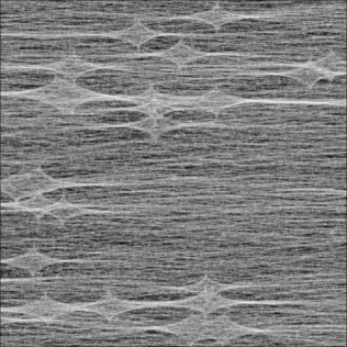
(a) 2% = M_⊙, 98% = 0.001000 M_⊙, total number of stars = 29887581

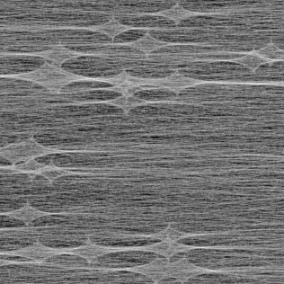
(b) 2% = M_⊙, 98% = 0.000675 M_⊙, total number of stars = 4920276

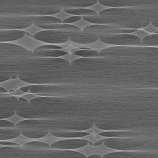
(c) 2% = M_⊙, 98% = 0.000025 M_⊙, total number of stars = 1195479475

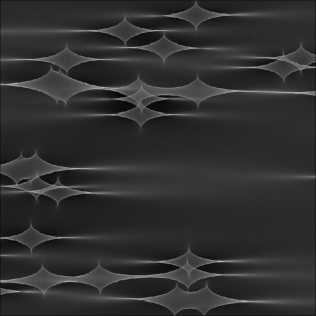
(d) 2% = M_⊙, 98% = Smooth, total number of stars = 609

Figure 4: Magnification maps from simulations of bi-modal mass distributions; these use the same parameters as figure 2 but use smaller and more numerous masses as the compact matter ($\sigma_{s}$). As the size of the masses is decreased the similarities between the use of compact masses (a)-(c) and smooth matter (d) become more marked.

Using our new implementation we can push down the mass size of the compact masses in bi-modal simulations, while at the same time increasing their number. Figure 4 shows simulations of quasar microlensing models that go down to 0.000025 M_⊙ for small compact mass objects; this is about 10 times Earth mass. Future simulations will go to smaller masses and possibly up to 3 billion stars. Of most interest is what happens to the magnification map as the masses become smaller. Figure 4 begins at case (c) of figure 2 and reduces the mass to 0.000025 M_⊙, increasing the number of stars to over a billion. With these small masses the large-scale caustics are becoming clearer and the fine-structure in-between the caustics is becoming smoother. Initial analysis indicates that as the small masses become smaller and more numerous the magnification distribution will tend to that of the smooth-matter case (d), but the size of the source will be important. Results of more complete investigations will be reported in forthcoming papers.

6 Discussion

Our new approach is of interest in itself, and can be studied as an instance of a large, parallel, computationally intensive implementation. Although our current aims excluded modifying the physics code, that can still be done at some later time.

6.1 Software Engineering

The following could be worthwhile scientific research projects based around our implementation:

Optimum distribution of rays to processors. Do rays that are close to clumps of matter really take longer to process than those that aren’t? And by how much? How close to optimal is our simple static load-distribution scheme?

Dynamic load balancing. Instead of fixing the allocation of rays to processors, the allocation could be varied at run-time, so that rays are moved from heavily loaded processors to lightly loaded processors. We could implement microtasking where each ray could be a task, with a scheduler pulling jobs off a run-queue and assigning them to processors for execution. We have not investigated whether the load on processors varies enough to warrant the overhead of dynamic load-balancing; our impressions are that it does not, for very large runs.

Distributed memory. A simulation of billions of stars generates hundreds of gigabytes of data, and this data has to go somewhere. If there are enough processes available with enough total memory, the data can be distributed amongst them and fetched across a network.

“Pre-set” stars. It would useful to generate stars and cells that can be saved and re-used, thus skipping the initialization phase altogether. A standard for the storing of lens/cell data could be developed by the lensing community, so that stars and cells can be stored and then simulated, modified, and re-used as necessary.

Multithreaded version. The new implementation has been built with this in mind. There is little data specific to a process that would have to be made specific to a thread; the significant shared data is external and can be accessed just the same by multiple threads or processes. Therefore a multithreaded version could be generated.

Use a commercial database for cells and stars. The assumption is that a commercial database will be more efficient at general file caching and perhaps can be tuned to the usage patterns of our simulations.

File compression. Compressing the stars and cell files on the fly will not make a simulation run faster, in fact it will run slower, but the data compresses to about 63% of its original size. This would be useful if we run short of disk space or go to bigger simulations, but particularly it could be useful for a distributed-memory version.

6.2 Science

Beyond computer engineering, there are the scientific aspects of simulating microlensing on computers, for example with the use of a cell tree. The cell tree is one reason why the original method executed so speedily, but it is also the reason for the huge amount of data generated. Instead of using a tree it may be possible to use other more recent models such as adaptive meshes that are used in N-body simulations (Yahagi, 2005).

There are also enhancements that can be made that add more physics to the implementation, such as implementing moving sources and moving stars. It is clear that both the source and the lens and the objects that make up the lens, if it is complex, are moving; and the gravitational potential and light curves are changing over time. The ability to simulate time-changing lensing events would be a significant advance over all current approaches.

7 Conclusion

We have generated a new version of a ray-shooting microlensing simulation tool that can be used to run huge simulations and continue research in quasar dark matter microlensing. We have discovered that the ray-shooting is easily parallelizable and simple load-balancing works well; parallelizing the stars and cell generation is not so easy, and memory caching could be improved with more research into the patterns of how the data is accessed.

Our new approach will now be used to continue research in microlensing; based on its performance and usefulness we can determine what modifications to pursue for the future.

8 Acknowledgements

We thank the anonymous reviewer for comments that improved the quality of this paper.

References

- Amri (2003) M. Amri, 2003. A New Data Distribution Method for Parallel Ray Tracing, in: E. Banissi, et al. (Eds.), Proc. 7th Int. Conf. Inf. Vis. (IV’03), IEEE Computer Society, London, pp. 79-84.
- Bate et al. (2008) N. F. Bate, R. L. Webster, J. S. B. Wyithe, 2008. Smooth Matter and Source Size in Microlensing Simulations of Gravitationally Lensed Quasars. MNRAS 381, 1591-1596.
- Blackburne et al. (2006) Blackburne, J. A., Pooley, D. & Rappaport, S., 2006. X-Ray and Optical Flux Anomalies in the Quadruply Lensed QSO 1RXS J1131-1231. ApJ, 640, 569.
- Brewer & Lewis (2008) Brewer, B. J., & Lewis, G. F. 2008. Unlensing HST observations of the Einstein ring 1RXS J1131-1231: a Bayesian analysis. MNRAS 390, 39-48.
- Chang & Refsdal (1979) Chang, K., & Refsdal, S., 1979. Flux variations of QSO 0957+561 A, B and image splitting by stars near the light path. Nature 282, 561-564.
- Chiba (2002) Chiba, M., 2002. Probing Dark Matter Substructure in Lens Galaxies. ApJ, 565, 17-23.
- Corrigan et al. (1990) Corrigan, R. T., Irwin, M. J., Hewett, P. C. & Webster, R. L. 1990. Photometric monitoring of 2237 + 0305, in: Gravitational lensing: Proceedings of a Workshop, Springer-Verlag, New York, pp. 206-209.
- Dalal & Kochanek (2002) Dalal, N. & Kochanek, C. S., 2002. Direct Detection of Cold Dark Matter Substructure. ApJ 572, 25-33.
- Deb et al. (2008) Deb, S., Goldberg, D. M., & Ramdass, V. J., 2008. Reconstruction of Cluster Masses Using Particle based Lensing. I. Application to Weak Lensing. ApJ 687, 39-49.
- Dye et al. (2008) Dye, S., Evans, N. W., Belokurov, V., Warren, S. J., & Hewett, P., 2008. Models of the Cosmic Horseshoe gravitational lens J1004+4112. MNRAS 388, 384-392.
- Eigenbrod et al. (2006) Eigenbrod, A., Courbin, F., Dye, S., Meylan, G., Sluse, D., Vuissoz, C., Magain, P., 2006. COSMOGRAIL: the COSmological MOnitoring of GRAvItational Lenses. II. SDSS J0924+0219: the redshift of the lensing galaxy, the quasar spectral variability and the Einstein rings. AA 451, 747-757.
- Glassner (1989) Glassner, A., 1989. An Introduction to Ray Tracing. Morgan Kaufman, San Francisco.
- Gaudi et al. (2008) Gaudi, B. S., et al., 2008. Discovery of a Jupiter/Saturn Analog with Gravitational Microlensing. Science 319, 927-+.
- Gunn et al. (1979) Gunn, J. E., Kristian, J., Oke, J. B., Westphal, J. A., Young, P. J., 1979. The Double Quasar Q0957+561. IAU Circ. 3431, 2-+.
- Huchra et al. (1985) Huchra, J., Gorenstein, M., Kent, S., Shapiro, I., Smith, G., Horine, E., Perley, R., 1985. 2237 + 0305 - A new and unusual gravitational lens. AJ 90, 691-696.
- Irwin et al. (1989) Irwin, M. J., Webster, R. L., Hewett, P. C., Corrigan, R. T., Jedrzejewski, R. I., 1989. Photometric variations in the Q2237 + 0305 system - First detection of a microlensing event. AJ 98, 1989-1994.
- Kayser et al. (1986) Kayser, R., Refsdal, S., & Stabell, R., 1986. Astrophysical applications of gravitational micro-lensing. A&A 166, 36-52.
- Keeton et al. (2006) Keeton, C. R., Burles, S., Schechter, P. L., Wambsganss, J., 2006. Differential Microlensing of the Continuum and Broad Emission Lines in SDSS J0924+0219, the Most Anomalous Lensed Quasar. ApJ, 639, 1-6.
- Kitching et al. (2008) Kitching, T. D., Miller, L., Heymans, C. E., van Waerbeke, L.,& Heavens, A. F., 2008. Bayesian galaxy shape measurement for weak lensing surveys - II. Application to simulations. MNRAS 390, 149-167.
- Knuth (1998) Knuth, D., 1998. The Art of Computer Programming Vol. 3, second ed. Addison-Wesley, Boston.
- Lee et al. (1998) Lee, T-Y., Raghavendra, C. S., Nicholas, J. B., 1998. Parallel implementation of a ray tracing algorithm for distributed memory parallel computers. Concurrency: Practice and Experience 9, 947-965.
- Lewis & Gil-Merino (2006) Lewis, G. F., & Gil-Merino, R., 2006. Quasar Microlensing: When Compact Masses Mimic Smooth Matter. ApJ 645, 835-840.
- Lewis & Ibata (2004) Lewis, G. F. & Ibata, R. A., 2004. Gravitational microlensing of quasar broad-line regions at large optical depths. MNRAS 348, 24-33.
- Mao & Schneider (1998) Mao, S., & Schneider, P., 1998. Evidence for substructure in lens galaxies? MNRAS 295, 587-+.
- Metcalf (2001) Metcalf, R. B., & Madau, P., 2001. Compound Gravitational Lensing as a Probe of Dark Matter Substructure within Galaxy Halos. ApJ 563, 9-20.
- Mortonson et al. (2005) Mortonson, M. J., Schechter, P. L., Wambsganss, J., 2005. Size Is Everything: Universal Features of Quasar Microlensing with Extended Sources. ApJ 628, 594-603.
- Myers et al. (1999) Myers, S. T., et al., 1999. CLASS B1152+199 and B1359+154: Two New Gravitational Lens Systems Discovered in the Cosmic Lens All-Sky Survey. AJ 117, 25652572.
- Ota et al. (2006) Ota, N., et al., 2006. Chandra Observations of SDSS J1004+4112: Constraints on the Lensing Cluster and Anomalous X-Ray Flux Ratios of the Quadruply Imaged Quasar. ApJ 647, 215-221.
- Paczynski (1986) Paczynski, B., 1986. Gravitational microlensing at large optical depth. Apj 301, 503-516.
- Pooley et al. (2006) Pooley, D., Blackburne, J. A., Rappaport, S., Schechter, P., Fong, W-f., 2006. A Strong X-Ray Flux Ratio Anomaly in the Quadruply Lensed Quasar PG 1115+080. ApJ 648, 67-72.
- Pooley et al. (2008) Pooley, D., Rappaport, S., Blackburne, J., Schechter, P. L., Schwab, J. & Wambsganss, J., 2008. The dark-Matter Fraction in the Elliptical Galaxy Lensing the Quasar PG 1115+080. ApJ, submitted.
- Reimers et al. (2002) Reimers, D., Hagen, H.-J., Baade, R., Lopez, S., Tytler, D., 2002. Discovery of a new quadruply lensed QSO: HS 0810+2554 - A brighter twin to PG 1115+080. A&A 352, L26-L28.
- Sand et al. (2008) Sand, D. J., Treu, T., Ellis, R. S., Smith, G. P., & Kneib, J.-P., 2008. Separating Baryons and Dark Matter in Cluster Cores: A Full Two-dimensional Lensing and Dynamic Analysis of Abell 383 and MS 2137-23. ApJ 674, 711-727.
- Schechter & Wambsganss (2002) Schechter, P., & Wambsganss, J., 2002. Quasar Microlensing at High Magnification and the Role of Dark Matter: Enhanced Fluctuations and Suppressed Saddle Points. ApJ 580, 685-695.
- Schneider et al. (1992) Schneider, P., Ehlers, J., & Falco, E. E. 1992. Gravitational Lenses. Springer-Verlag, New York.
- Turner et al. (1989) Turner, E. L. et al., 1989. MG0414+0534: A Candidate Gravitational Lens. BAAS 21, 718-+.
- Vanderriest et al. (1983) Vanderriest, C., Wlerick, G., Felenbok, P., 1983. PG 1115+080. IAU Circ. 3841, 3-+.
- Verdu et al. (1996) Verdú, I., Giménez, D. & Torres, J. C., 1996. Ray Tracing for natural scenes in parallel processors, in: Liddell, H. M., Colbrook, A., Hertzberger, B., Sloot, P. (Eds.), Proc. Int. Conf. High-Performance Computing and Networking. Springer, Italy, pp. 297-305.
- Walsh et al. (1979) Walsh, D., Carswell, R. F. & Weymann, R. J., 1979. 0957 + 561 A, B - Twin quasistellar objects or gravitational lens. Nature 279, 381-384.
- Wambsganss (1990) Wambsganss, J., 1990. Ph.D. thesis, Univ. of Munich (Report MPA 550).
- Wambsganss & Paczynski (1991) Wambsganss, J., Paczynski, B., 1991. Expected color variations of the gravitationally microlensed QSO 2237 + 0305. AJ 102, 864-868.
- Wambsganss (1992) Wambsganss, J., 1992. Probability distributions for the magnification of quasars due to microlensing. ApJ 386, 19-29.
- Wambsganss (1999) Wambsganss, J., 1999. Gravitational lensing: numerical simulations with a hierarchical tree code. J. Comput. Appl. Math. 109, 353-372.
- Wang et al. (2009) Wang, S., Haiman, Z., May, M., 2009. Constraining Cosmology with High-Convergence Regions in Weak Lensing Surveys. ApJ 691, 547-559.
- Witt et al. (1995) Witt, H. J., Mao, S., & Schechter, P., 1995. On the universality of microlensing in quadruple gravitational lenses. ApJ 443, 18-28.
- Udalski et al. (2006) Udalski, A. et al., 2006. The Optical Gravitational Lensing Experiment. OGLE-III Long Term Monitoring of the Gravitational Lens QSO 2237+0305. Acta Astronomica 56, 293-305.
- Yahagi (2005) Yahagi, H., 2005. Vectorization and Parallelization of the Adaptive Mesh Refinement N-body Code. PASJ 57, 779-798.
- Young (1981) Young, P., 1981. Q0957+561 - Effects of random stars on the gravitational lens. ApJ 244, 756-767.