On the Continuity of Stochastic Exit Time Control Problems

Abstract.

We determine a weaker sufficient condition than that of Theorem 5.2.1 in Fleming and Soner (2006) for the continuity of the value functions of stochastic exit time control problems.

Keywords and Phrases. Continuity of the value function, exit time control, degenerate diffusions, viscosity solutions, the Cauchy problem on bounded domains.

AMS subject classifications. 60G20, 93E15.

1. Introduction

Let $(\Omega,\mathcal{F},\mathbb{F}=(\mathcal{F}_{s})_{t\leq s<\infty},\mathbb{P})$ be a filtered probability space satisfying the usual conditions and $W$ be an $\mathbb{R}^{d}$ valued Brownian motion adapted to $\mathbb{F}$. Consider the following stochastic differential equation in $\mathbb{R}^{n}$

$$dX_{s}=b(s,X_{s},\alpha_{s})ds+\sigma(s,X_{s},\alpha_{s})dW_{s},\quad$$ (1.1)

where $\alpha_{t}$ the control belongs to $\mathcal{A}$, the set of all progressively measurable processes with values in a compact subset $A$ of $\mathbb{R}^{k}$.

Let $O\subset\mathbb{R}^{n}$ be a bounded open set, and set $Q=[0,T)\times O$. For a given initial $(t,x)\in Q$, define $\tau$ as the first exit time of the $\mathbb{R}^{n+1}$-valued process $(s,X_{s})$ from the bounded domain $Q$, that is

$$\tau=\inf\{s\geq t:(s,X_{s})\notin Q\}.$$ (1.2)

Given a running cost function $\ell:\mathbb{R}_{+}\times\mathbb{R}^{n}\times A\to\mathbb{R}$ and a terminal cost function $g:\mathbb{R}_{+}\times\mathbb{R}^{n}\to\mathbb{R}$, we define the value function as

$$V(t,x)=\inf_{\alpha\in\mathcal{A}}\mathbb{E}_{t,x}\left\{\int_{t}^{\tau}\ell(s,X_{s},\alpha_{s})ds+g(\tau,X(\tau))\right\},$$ (1.3)

in which $\mathbb{E}_{t,x}$ is the expectation operator conditional on $X_{t}=x$. Occasionally, we will refer to $X$ as $X^{t,x}$ to emphasize its initial condition.

In general one can show that the value function is a viscosity solution of a fully non-linear Hamilton-Jacobi-Bellman equation given that it is a continuous function; see Corollary 3.1 on page 209 of [4]. However, when the domain is bounded, it is not always the case that the value function is continuous due to tangency problem mentioned in [11, pp. 278-279], which imposes continuity as an additional assumption. Consider two underlying processes $X^{1}=X^{t,x^{1}}$ (solid line) and $X^{2}=X^{t,x^{2}}$ (dotted line) in Figure 1. No matter how close $X^{1}$ and $X^{2}$ are, the difference between their first exit time $\tau_{1}$ and $\tau_{2}$ could be very large.

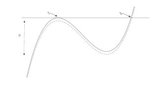
Figure 1. Tangency problem

A sufficient condition for the continuity of the value function is provided on page 205 of [4]. In this paper we improve this condition using a probabilistic argument; see Theorem 4.1 and Example 4.1. We also note that the regularity of the stochastic exit time control problem has been studied in [12], in which the value function is shown to be Lipschitz continuous assuming the existence of an appropriate “global barrier”. Under weaker assumptions, similar to the ones considered here, the continuity of the value function was obtained by [1] and [6] for semi-linear and quasi-linear Dirichlet problems, respectively, using purely PDE methods. More recently, the continuity of viscosity solutions of fully non-linear Dirichlet problems (with integro-differential terms) is analyzed in [2]. Related results can also be found in [8], where the Dirichlet problem for the Isaacs Equation is discussed. With respect to these aforementioned papers our contribution is to give a simple probabilistic proof of the continuity result for the fully nonlinear Cauchy problems on bounded domains.

The rest of the paper is organized as follows: In Section 2 we recall some preliminary results. Section 3, is devoted to an important result on the sample path behavior of the state process on the boundary of the domain of the problem. Using the results developed in Section 3, a sufficient condition on the continuity of the value function is derived in Section 4. Some of the proofs are given in the Appendix.

2. Preliminaries

This section presents definitions and assumptions needed for the setup of our problem, and collects some relevant classical results.

To proceed, we present the standing assumptions needed for our work. Below we use $|\cdot|$ for the absolute value of a scalar and $\|\cdot\|$ for the second Euclidean norm.

Assumption 2.1.

For any $x,x^{1},x^{2}\in\mathbb{R}^{n}$, $a\in A$, $t\in[0,T]$, functions $b,\sigma,\ell$, and $g$ satisfy, for some strictly positive constant $K$

1. $\|b(t,x^{1},a)-b(t,x^{2},a)\|+\|\sigma(t,x^{1},a)-\sigma(t,x^{2},a)\|\leq K{\|x^{1}-x^{2}\|};$

2. $\|b(t,x,a)\|+\|\sigma(t,x,a)\|\leq K(1+\|x\|)$, $\forall(t,x,a)\in[0,T]\times\mathbb{R}^{n}\times A$;

3. $\ell$ and $g$ are continuous functions;

4. $|\ell(t,x^{1},a)-\ell(t,x^{2},a)|+|g(t,x^{1})-g(t,x^{2})|\leq K{\|x^{1}-x^{2}\|};\;x^{1},x^{2}\in\mathbb{R}^{n},(t,a)\in[0,T]\times A;$

5. $|\ell(t,x,a)|+|g(t,x)|\leq K(1+\|x\|^{2})$.

The first two of our assumptions guarantee that (1.1) has a unique strong solution for a given $\alpha\in\mathcal{A}$.

Next, we present the dynamic programming principle; see e.g. [4, 13].

Proposition 2.1.

For any stopping time $\theta$ with $t\leq\theta\leq\tau$,

$$V(t,x)=\inf_{\alpha\in\mathcal{A}}\mathbb{E}_{t,x}\left\{\int_{t}^{\theta}\ell(s,X_{s},\alpha_{s})ds+V(\theta,X_{\theta})\right\}.$$ (2.1)

Let $\forall\varphi\in C^{1,2}(Q)$

$$G^{a}\varphi(t,x)=\varphi_{t}(t,x)+L_{t}^{a}\varphi(x),$$

and

$$L_{t}^{a}\varphi(x)=b(t,x,a)\cdot D_{x}\varphi(t,x)+\frac{1}{2}\hbox{ tr }(\sigma\sigma^{\prime}(t,x,a)D_{x}^{2}\varphi(t,x)).$$ (2.2)

Using the dynamic programming principle it can be seen that the value function is a solution of

$$\begin{split}\inf_{a\in A}\{G^{a}V(t,x)+\ell(t,x,a)\}&=0,\quad(t,x)\in Q,\\ V(t,x)&=g(t,x),\quad(t,x)\in\partial^{*}Q\triangleq[0,T)\times\partial O\cup\{T\}\times O,\end{split}$$ (2.3)

in the sense, which we will now describe.

Definition 2.1.

Let $u(t,x)=g(t,x)$, $(t,x)\in\partial^{*}Q$. (i) It is called a viscosity subsolution of (2.3) if for any $(t_{0},x_{0};\varphi)\in Q\times C^{2,1}(Q)$ such that $\varphi(t,x)\leq u(t,x)$, $(t,x)\in Q$, and $\varphi(t_{0},x_{0})=u(t_{0},x_{0})$ we have that

$$\inf_{a\in A}\left\{G^{a}\varphi(t_{0},x_{0})+\ell(t_{0},x_{0},a)\right\}\geq 0.$$

(ii) It is called a viscosity supersolution of (2.3) if for any $(t_{0},x_{0};\varphi)\in Q\times C^{2,1}(Q)$ such that $\varphi(t,x)\geq u(t,x)$, $(t,x)\in Q$, and $\varphi(t_{0},x_{0})=u(t_{0},x_{0})$ we have that

$$\inf_{a\in A}\left\{G^{a}\varphi(t_{0},x_{0})+\ell(t_{0},x_{0},a)\right\}\leq 0.$$

(iii) Finally, $u$ is a viscosity solution if it is both a viscosity subsolution and a viscosity supersolution.

Proposition 2.2.

Suppose $V(t,x)\in C(\bar{Q})$ and Assumption 2.1 hold. Then the value function $V(t,x)$ is the unique viscosity solution of (2.3).

A complete proof of Proposition 2.2 can be found in [4]. In Appendix, we provide an alternative proof for the existence part.

The characterization of the value function in Proposition 2.2 assumes that it is continuous. However the value function is not necessarily continuous if the domain is a bounded set (see Figure 1 and Example 4.1). In the next section we give a sufficient condition that guarantees the continuity of the value function. This improves on the condition provided in Section V.2 of [4].

3. Sample Path Behavior on the boundary of domain

In this section, we will discuss the sample path behavior of Itô process on $[0,T)\times\partial O$, which turns out to be crucial for the continuity of the value function.

For a given constant vector $a\in A$, let $Y$ be the unique strong solution of the following stochastic differential equation:

$$dY_{s}=b(s,Y_{s},a)ds+\sigma(s,Y_{s},a)dW_{s},\quad Y_{t}=y.$$

The main result of this section, which we will state next, derives a sufficient condition (3.2), under which the process $Y$ must hit $\bar{O}^{c}$ infinitely many times in any small duration, if it starts on $\partial O$. To formulate our result, let us denote the signed distance function by

$$\hat{\rho}(y)\triangleq\begin{cases}\hbox{dist}(y,\bar{O}),&y\notin O;\\ -\hbox{dist}(y,{O^{c}}),&y\in O.\end{cases}$$ (3.1)

Proposition 3.1.

Let $(t,y)\in[0,T)\times\partial O$ and $a\in A$. Assume that $\partial O\in C^{2}$ and that

$$\max\{L_{t}^{a}\hat{\rho}(y),\|\sigma^{\prime}(t,y,a)D\hat{\rho}(y)\|\}>0.$$ (3.2)

Then,

$$\inf\{s>t:Y_{s}\notin\bar{O}\}=t\quad\mathbb{P}-\text{a.s.}$$ (3.3)

Remark 3.1.

The assumption that $\partial O\in C^{2}$ implies that $\hat{\rho}\in C^{2}$ in a neighborhood of $\partial{O}$; see Lemma 14.16 in [5]. Also see page 78 of [9] and the references therein.

Before we present the proof of this proposition, we will need some preparation. First, note that (3.3) can be written as the local behavior of a one-dimensional process $\hat{\rho}(X_{s})$:

$$\inf\{s>t:\hat{\rho}(Y_{s})>0\}=t\quad\mathbb{P}-a.s.$$

Next, we will focus on one-dimensional process, which implies that a non-degenerate continuous local martingale process $M$ starting from zero hits $(0,\infty)$ infinitely many times in any small time period. If $M$ is a standard Brownian motion, the proof is given by Blumenthal 0-1 law [3, Theorem 7.2.6]. However, because the distribution of $M$ is not explicitly available, we use the representation of $M$ as a time changed Brownian motion.

Lemma 3.1.

Let $\hat{B}(r)$ be a one-dimensional Brownian motion with respect to $(\Omega,\mathcal{F},\mathbb{F},\mathbb{Q})$. We assume that $\hat{\sigma}$ is a one-dimensional progressively measurable process with $\int_{t}^{T}\hat{\sigma}_{r}^{2}dr<\infty$, so that $M_{s}=\int_{t}^{s}\hat{\sigma}_{r}d\hat{B}_{r}$ is a local martingale. Furthermore, we assume that $\hat{\sigma}_{s}>0$ $\forall s\in[t,T]$ $\mathbb{Q}$-a.s. Then $\tau=\inf\{s>t:M_{s}>0\}$ satisfies $\tau=t$ $\mathbb{Q}$-a.s.

Proof.

First, we can extend function $\hat{\sigma}$ on $[t,T]$ to $[t,\infty)$ by $\hat{\sigma}(s)=\hat{\sigma}(T)$ for all $s>T$. Then, the quadratic variation of $M$ is a strictly increasing function and it satisfies

$$\langle M\rangle_{s}=\int_{t}^{s}\hat{\sigma}^{2}(r)dr\to\infty\hbox{ as }s\to\infty,\ \mathbb{Q}-a.s.$$

since $\hat{\sigma}>0$. For a given positive $s$, define $T(s)\triangleq\inf\{r\geq 0:\langle M\rangle(r)>s\}.$ The strictly increasing function $T$ satisfies $T\left(\langle M\rangle(s)\right)=s.$ The time-changed process $B_{s}\triangleq M_{T(s)}$ is a $\mathbb{Q}$-Brownian motion under the filtration $\mathcal{G}_{s}=\mathcal{F}_{T(s)}$ and $M_{s}=B_{\langle M\rangle(s)}$; see e.g. [7, Theorem 3.4.6]. Thus, $\mathbb{Q}$-almost surely, we have

$$\begin{array}[]{ll}\inf\{s:M_{s}>0\}&=\inf\{s:B_{\langle M\rangle(s)}>0\}\\ &=\inf\{T\left(\langle M\rangle(s)\right):B_{\langle M\rangle(s)}>0\}\\ &=T\left(\inf\{\langle M\rangle(s):B_{\langle M\rangle(s)}>0\}\right)\\ &=T(0)=0.\end{array}$$

The second equality follows from the fact that $\hat{\sigma}>0$. The third, on the other hand, follows from the fact that $T$ is increasing. ∎

We are ready to prove Proposition 3.1.

Proof of Proposition 3.1.

We will carry out the proof in two steps.
(i) Let us first assume that $\|\sigma^{\prime}(t,y,a)D\hat{\rho}(y)\|>0$. Due to the continuity of this function, there exists a stopping time $\tau>t$, (which is less than the exit time from the neighborhood mentioned in Remark 3.1) such that for $s\in(t,\tau)$

$$\|\sigma^{\prime}(s,Y_{s},a)D\hat{\rho}(Y_{s})\|>\varepsilon\triangleq\frac{1}{2}\|\sigma^{\prime}(t,y,a)D\hat{\rho}(y)\|>0,\quad\mathbb{P}-a.s.$$ (3.4)

Thus, applying Itô’s formula, we obtain

$$\begin{array}[]{ll}\hat{\rho}(Y_{s})&\displaystyle=\int_{t}^{s}L_{r}^{a}\hat{\rho}(Y(r))dr+\int_{t}^{s}D\hat{\rho}(Y(r))\sigma(r,Y(r),a)dW(r)\\ &=\displaystyle\int_{t}^{s}L_{r}^{a}\hat{\rho}(Y(r))dr+\int_{t}^{s}\|\sigma^{\prime}(r,Y(r),a)D\hat{\rho}(Y(r))\|d\widetilde{W}(r)\end{array}$$

where $\widetilde{W}$ is a one-dimensional $\mathbb{P}$-Brownian motion. By Girsanov’s theorem, there exists $\mathbb{Q}\sim\mathbb{P}$, such that

$$\begin{array}[]{ll}\hat{\rho}(Y_{s})\displaystyle=\int_{t}^{s}\|\sigma^{\prime}(r,Y(r),a)D\hat{\rho}(Y(r))\|d\widetilde{W}_{r}^{\mathcal{Q}}\end{array}$$

where $\widetilde{W}_{r}^{\mathcal{Q}}$ is a $\mathbb{Q}$-Brownian motion. Thus, $\hat{\rho}(Y_{s})$ is a local martingale process under $\mathbb{Q}$. Lemma 3.1 implies that

$$\inf\{s>t:\hat{\rho}(Y_{s})>0\}=t,\quad\mathbb{Q}-\text{a.s.}$$

Since $\mathbb{P}$ is equivalent to $\mathbb{Q}$, and the conclusion holds $\mathbb{P}$-a.s.

(ii) This was a case already proved in [4, Lemma V.2.1]. ∎

4. Continuity of the value function

We will construct a sequence of functions that converge uniformly to the value function. For this purpose let $\hat{d}(x)=\hat{\rho}^{+}(x)$ and define $\Lambda^{\varepsilon}(s,X)\triangleq\displaystyle\exp\left\{-\frac{1}{\varepsilon}\int_{t}^{s}\hat{d}(X_{r})dr\right\}.$ Let

$$J^{\varepsilon}(t,x,\alpha)=\mathbb{E}_{t,x}\left\{\int_{t}^{T}\Lambda^{\varepsilon}(s,X)\ell(s,X_{s},\alpha_{s})ds+\Lambda^{\varepsilon}(T,X)g(T,X(T))\right\}.$$ (4.1)

and

$$\begin{array}[]{ll}V^{\varepsilon}(t,x)=\inf_{\alpha\in\mathcal{A}}J^{\varepsilon}(t,x,\alpha).\end{array}$$ (4.2)

Next, Lemma 4.1 shows the continuity of this function. Its proof is given in the Appendix.

Lemma 4.1.

Under Assumption 2.1, $V^{\varepsilon}\in C([0,T]\times\bar{O})$. In fact,

$$\begin{array}[]{ll}|V^{\varepsilon}(t_{1},x^{1})-V^{\varepsilon}(t_{2},x^{2})|\leq C_{\varepsilon}(\|x^{1}-x^{2}\|+|t_{1}-t_{2}|^{1/2}),\end{array}$$

for some positive constant $C_{\varepsilon}$.

Theorem 4.1.

Assume that Assumption 2.1 and the following hold:

1. $\partial O\in C^{2}$;

2. $\forall(t,x)\in[0,T)\times\partial O$, there exists an $a\in A$ satisfying (3.2);

3. $$\inf_{a\in A}\{G^{a}(u+g)(t,x)+\ell(t,x,a)\}\geq 0,\forall(t,x)\in[0,T]\times\mathbb{R}^{n}.$$ (4.3)

Then $V$ is continuous on $\bar{Q}$.

Remark 4.1.

In [4, Pages 202-203], a sufficient condition for the continuity of the value function is given: $L_{t}^{a}\hat{\rho}(y)>0$ for some $a\in A$ for all $(t,y)\in[0,T)\times\partial O$. Theorem 4.1 provides an alternative sufficient condition: $\|\sigma^{\prime}(t,x,a)D\hat{\rho}(x)\|>0$ for some $a\in A$ for all $(t,x)\in[0,T)\times\partial O$.

Proof.

The proof is divided into two steps.

(i) Assume that $\ell\geq 0,g=0$ on $\mathbb{R}_{+}\times\mathbb{R}^{n}\times A$. Fix $(t,x)\in[0,T)\times\partial O$. Let $a\in A$ satisfy (3.2). Consider the constant control process $\{a_{s}\equiv a:s\geq t\}$ and let $Y$ denote the corresponding process governed by this constant control. By Theorem 3.1 for $s\in(t,T]$ we have

$$\begin{array}[]{ll}\displaystyle\int_{t}^{s}\hat{d}(Y_{r})dr>0,\quad\mathbb{P}-\text{a.s.}\end{array}$$

Hence,

$$\begin{array}[]{ll}\lim_{\varepsilon\to 0^{+}}\Lambda^{\varepsilon}(s,Y)=0\quad\mathbb{P}-a.s.\end{array}$$

By Dominated Convergence Theorem, one can conclude that

$$\begin{array}[]{ll}\lim_{\varepsilon\to 0^{+}}\mathbb{E}_{t,x}\left\{\int_{t}^{T}\Lambda^{\varepsilon}(s,Y)\ell(s,Y_{s},a)ds+\Lambda^{\varepsilon}(T,Y)g(T,Y_{T})\right\}=0.\end{array}$$

This implies

$$\lim_{\varepsilon\to 0^{+}}J^{\varepsilon}(t,x,a)=0.$$

Together with $J^{\varepsilon}(t,x,a)\geq V^{\varepsilon}(t,x)\geq 0$ which follows from (4.2), the above implies that

$$\lim_{\varepsilon\to 0^{+}}V^{\varepsilon}(t,x)=0=V(t,x),\quad(t,x)\in[0,T]\times\partial O.$$ (4.4)

Therefore, $V^{\varepsilon}(t,x)$ is continuous (Lemma 4.1) on the compact set $[0,T]\times\partial O$ in $\mathbb{R}^{n+1}$, and it monotonically converges to the zero function. Dini’s theorem implies that $\lim_{\varepsilon\to 0^{+}}V^{\varepsilon}(t,x)=0$ uniformly on $[0,T]\times\partial O$. Thanks to the uniform convergence, if we set

$$\begin{array}[]{ll}h(\varepsilon)\triangleq\sup\{V^{\varepsilon}(t,x):(t,x)\in[0,T]\times\partial O\},\end{array}$$

we have that $\lim_{\varepsilon\to 0^{+}}h(\varepsilon)=0$.

Now we are ready to prove the continuity of the value function $V$. Let $(t,x)\in Q$. Applying the dynamic programming principle to $V^{\varepsilon}(\cdot,\cdot)$ with respect to stopping time $\tau$ of (1.2), and using the fact that $\Lambda^{\varepsilon}(s,X_{s}^{t,x,\alpha},\alpha_{s})\equiv 1$ for $s\leq\tau$ and $\alpha\in\mathcal{A}$, we obtain

$$\begin{array}[]{ll}V^{\varepsilon}(t,x)&\displaystyle=\inf_{\alpha\in\mathcal{A}}\left\{\mathbb{E}_{t,x}\left[\int_{t}^{\tau}\ell(s,X_{s}^{t,x,\alpha},\alpha_{s})ds+V^{\varepsilon}(\tau,X^{t,x,\alpha}_{\tau})\right]\right\}\\ &\leq\displaystyle\inf_{\alpha\in\mathcal{A}}\left\{\mathbb{E}\left[\int_{t}^{\tau}\ell(s,X^{t,x,\alpha}_{s},\alpha_{s})ds\right]\right\}+h(\varepsilon),\quad\hbox{ since }(\tau,X^{t,x,\alpha}_{\tau})\in\partial^{*}Q\\ &=V(t,x)+h(\varepsilon).\end{array}$$ (4.5)

Since $\ell\geq 0$, we further have that

$$\begin{array}[]{ll}V(t,x)\leq V^{\varepsilon}(t,x)\leq V(t,x)+h(\varepsilon),\ \forall(t,x)\in\bar{Q}\end{array}$$

This implies $V^{\varepsilon}\to V$ uniformly on $\bar{Q}$. Since $V^{\varepsilon}$ is continuous by Lemma 4.1, the value function $V$ is also continuous.

(ii) The proof follows from (i) once we let $\tilde{l}(t,x,a)\triangleq l(t,x,a)+G^{a}g(t,x)$ and consider (1.3) and (4.2) by setting $l=\tilde{l}$ and $g=0$.

∎

Next, we give an example, whose value function is continuous, although it does not satisfy the sufficient condition of [4]. In this example, we first consider a deterministic exit time problem. We observe that this problem does not have a continuous value function. Next, we consider a degenerate random version of the same problem. In this problem, the sufficient condition $L_{t}^{a}\hat{\rho}(x)>0$ of [4] holds only for some points $x$ on the boundary. Yet, it still satisfies the sufficient condition of (3.2) on the entire boundary, and therefore, the value function is continuous.

Example 4.1.

(i) Let $X^{t,x}_{s}$, $s\geq t$, be the one-dimensional process satisfying

$$dX^{t,x}_{s}=-2(s-1)ds,\ X^{t,x}_{t}=x.$$

Let $Q=[0,2)\times(-1,1)$, and $\tau^{t,x}=\inf\{s>t:X^{t,x}(s)\notin(-1,1)\}$. Let us define the value function as $V(t,x)=(\tau^{t,x}\wedge 2)-t$. Then, $X^{t,x}$ has an explicit form:

$$X^{t,x}_{s}=-(s-1)^{2}+x+(t-1)^{2}.$$

Therefore, the function $s\to X_{s}^{t,x}$ first increases towards its maximum

$$\max_{s\geq t}X^{t,x}_{s}=x+(t-1)^{2},$$

and upon reaching it decreases to $-\infty$. Thus, if $x+(t-1)^{2}\geq 1$, then $X^{t,x}_{\tau^{t,x}}=1$, otherwise $X^{t,x}_{\tau^{t,x}}=-1$. As a result, for $t\in[0,1]$, $V(t,x)$ is discontinuous at every point on the parabola

$$\left\{(t,x)\in Q:\max_{s\geq t}X_{s}=1\right\}=\left\{(t,x)\in Q:x=-t^{2}+2t\right\}.$$

We also note that, (3.2) does not hold, since

$$\max\{L^{a}_{t}\hat{\rho}(\pm 1),\|\sigma^{\prime}(t,x,a)\hat{\rho}(\pm 1)\|\}=0,\quad\forall t\in(0,1).$$

(ii) Next, we consider the following state process, which we obtain by adding a random perturbation to the above deterministic process:

$$dX^{t,x}_{s}=-2(s-1)ds+(2s-X_{s}^{t,x})^{+}dW_{s},\ X^{t,x}_{t}=x.$$

This equation admits a unique strong solution since the coefficients are Lipschitz continuous. Let us define the value function to be $V(t,x)\triangleq\mathbb{E}_{t,x}[(\tau^{t,x}\wedge 2)-t]$. Note that, $\hat{\rho}(\cdot)$ of (3.1) satisfies

$$\hat{\rho}(x)=(x-1){\hbox{1{\kern-3.50006pt}1}}_{\{x\geq 0\}}+(-1-x){\hbox{1{\kern-3.50006pt}1}}_{\{x<0\}},\ D\hat{\rho}(x)=\mathop{sgn}(x),\hbox{ and }D^{2}\hat{\rho}(x)\equiv 0.$$ (4.6)

As a result,

$$L_{t}\hat{\rho}(1)=-2(t-1)>0\hbox{ on }t\in(0,1);\quad|\sigma(t,1)D\hat{\rho}(1)|=(2t-1)^{+}>0\hbox{ on }t\in(1/2,2),$$

and

$$L_{t}\hat{\rho}(-1)=2(t-1)>0\hbox{ on }t\in(1,2);\quad|\sigma(t,1)D\hat{\rho}(-1)|=(2t+1)^{+}>0\hbox{ on }t\in(0,2).$$

Although, the condition $L_{t}^{a}\hat{\rho}>0$, which is the sufficient condition given by [4]—see equation (2.8) on page 202— fails on the boundary, the continuity of the value function follows from Theorem 4.1. ∎

5. Appendix

5.1. Proof of Proposition 2.2

First, we will develop the following auxiliary result.

Lemma 5.1.

For a given $(t,x)\in Q$, define

$$\theta=\inf\{s>t:(s,X_{s})\notin[t,t+h^{2})\times B(x,h)\},$$

where $B(x,h)$ is a ball centered at $x$ with radius $h\in(0,1)$. Then, there exists a constant $K$, which does not depend on the control $\alpha$, such that

$$\begin{array}[]{ll}\mathbb{E}_{t,x}[\theta-t]\geq Kh^{2}.\end{array}$$

Proof.

Let $f(y)=\|y-x\|^{2}$. Applying Itô’s formula and taking expectations yield

$$\mathbb{E}_{t,x}\{f(X_{\theta})-f(x)\}=\mathbb{E}_{t,x}\left\{\int_{t}^{\theta}L_{s}^{\alpha_{s}}f(X_{s})ds\right\}.$$ (5.1)

Since $[t,t+1]\times\bar{B}(x,1)\times A$ is compact, by continuity

$$\begin{array}[]{ll}\displaystyle\sup_{(s,x,a)\in[t,t+1]\times\bar{B}(x,1)\times A}|L_{s}^{a}f(x)|\leq K_{t,x}<\infty,\end{array}$$

for some constant $K_{t,x}$. Since $(s,X_{s},\alpha_{s})\in[t,t+1]\times\bar{B}(x,1)\times A$ for any $s\in[t,\theta]$ the integrand in (5.1) is bounded above by $K_{t,x}$. Since $f(x)=0$, we can write (5.1) as

$$\mathbb{E}_{t,x}\left[{\hbox{1{\kern-3.50006pt}1}}_{\{\theta=t+h^{2}\}}f(X_{\theta})\right]+\mathbb{E}_{t,x}\left[{\hbox{1{\kern-3.50006pt}1}}_{\{\theta<t+h^{2}\}}h^{2}\right]=\mathbb{E}_{t,x}\left[\int_{t}^{\theta}L^{\alpha_{s}}f(X_{s})ds\right]\leq K_{t,x}\mathbb{E}_{t,x}\left[\theta-t\right].$$

On the other hand,

$$\begin{array}[]{ll}\mathbb{E}_{t,x}[\theta-t]\geq\mathbb{E}_{t,x}\left[(\theta-t){\hbox{1{\kern-3.50006pt}1}}_{\{\theta=t+h^{2}\}}\right]=h^{2}\mathbb{E}_{t,x}\left[{\hbox{1{\kern-3.50006pt}1}}_{\{\theta=t+h^{2}\}}\right].\end{array}$$

Adding the last two inequalities, we get

$$\begin{array}[]{ll}(K_{t,x}+1)\mathbb{E}_{t,x}[\theta-t]\geq h^{2}+\mathbb{E}_{t,x}\left[{\hbox{1{\kern-3.50006pt}1}}_{\{\theta=t+h^{2}\}}f(X_{\theta})\right]\geq h^{2}.\end{array}$$

The result follows by setting $K\triangleq 1/(K_{t,x}+1)$. ∎

Now, we are ready to prove Proposition 2.2.

Proof of Proposition 2.2.

(i) We will first show that $V$ is a subsolution of (2.3). We will prove the assertion by a contradiction argument. Let us assume that there $(t,x;\varphi)$ as in Definition 2.1-(i) such that

$$\ell(t,x,a)+G^{a}\varphi(t,x)<-\delta,$$

for some $\delta>0$. Then, by continuity of $\ell+G^{a}\varphi$ in $(t,x)$, there exists $h>0$ such that

$$\ell(s,y,a)+G^{a}\varphi(y,a)<-\frac{\delta}{2}<0,\quad\forall(s,y)\in[t,t+h^{2})\times B(x,h)\subset Q.$$

Let $Y$ be the process which can be obtained by applying the control $\alpha\equiv a$ and define

$$\theta=\inf\{s>t,Y_{s}\notin B(x,h)\}\wedge(t+h^{2}).$$

By the dynamic programing principle

$$V(t,x)\leq\mathbb{E}_{t,x}\left\{\int_{t}^{\theta}\ell(s,Y_{s},a)ds+V(\theta,Y_{\theta})\right\}.$$

It follows from how $\varphi$ is chosen that

$$\begin{array}[]{ll}0&\leq\displaystyle\mathbb{E}_{t,x}\left\{\int_{t}^{\theta}\ell(s,Y_{s},a)ds+\varphi(\theta,Y_{\theta})-\varphi(t,x)\right\}\\ &=\displaystyle\mathbb{E}_{t,x}\left\{\int_{t}^{\theta}[\ell(s,Y_{s},a)+G^{a}\varphi(s,Y_{s})]ds\right\}<-\mathbb{E}_{t,x}\left\{\int_{t}^{\theta}\left(\frac{\delta}{2}\right)ds\right\}<0,\end{array}$$

which yields a contradiction.

(ii) We will now show that $V$ is a supersolution of (2.3). We will, again, use proof by contradiction. Let us assume that there exists a triplet $(t,x;\varphi)$ as in Definition 2.1-(ii) such that

$$\inf_{a\in A}\{\ell(t,x,a)+G^{a}\varphi(t,x)\}=\delta>0,$$

As a function of $(t,x)$, $\ell(t,x,a)+G^{a}\varphi(t,x)$ is equicontinuous in $A$, by Assumption 2.1. Therefore,

$$\inf_{a\in A}\{\ell(t,x,a)+G^{a}\varphi(t,x)\}$$

is also continuous in $(t,x)$. So, one can find $h>0$ such that

$$\inf_{a\in A}\{\ell(s,y,a)+G^{a}\varphi(s,y)\}>\frac{\delta}{2}>0,\quad\forall(s,y)\in[t,t+h^{2})\times B(x,h).$$

Let $\varepsilon=\frac{\delta}{4}Kh^{2}$, where $K$ is the constant in Lemma 5.1. Let $\alpha$ be $\varepsilon$-optimal control and define

$$\theta=\inf\{s>t:X_{s}\notin B(x,h)\}\wedge(t+h^{2}).$$

Then

$$\begin{array}[]{ll}V(t,x)&\displaystyle\geq\mathbb{E}_{t,x}\left\{\int_{t}^{\tau}\ell(s,X_{s},\alpha_{s})ds+g(\tau,X_{\tau})\right\}-\varepsilon\\ &\displaystyle\geq\mathbb{E}_{t,x}\left\{\int_{t}^{\theta}\ell(s,X_{s},\alpha_{s})ds+V({\theta},X_{\theta})\right\}-\varepsilon,\end{array}$$

In the following, we obtain the desired contradiction:

$$\begin{array}[]{ll}0&\displaystyle\geq\mathbb{E}_{t,x}\left\{\int_{t}^{\theta}\ell(s,X_{s},\alpha_{s})ds+\varphi({\theta},X_{\theta})-\varphi(t,x)\right\}-\varepsilon,\\ &\displaystyle=\mathbb{E}_{t,x}\left\{\int_{t}^{\theta}[\ell(s,X_{s},\alpha_{s})+G^{\alpha_{s}}\varphi(s,X_{s})]ds\right\}-\varepsilon\\ &\displaystyle\geq\mathbb{E}_{t,x}\left\{\int_{t}^{\theta}[\ell(s,X_{s},\alpha_{s})+G^{\alpha_{s}}\varphi(s,X_{s})]ds\right\}-\frac{\delta}{4}\mathbb{E}_{t,x}[{\theta}-t],\quad\hbox{ by Lemma~{}{\rm\ref{l-estop}}}\\ &\displaystyle=\mathbb{E}_{t,x}\left\{\int_{t}^{\theta}\left[\ell(s,X_{s},\alpha_{s})+G^{\alpha_{s}}\varphi(s,X_{s})-\frac{\delta}{4}\right]ds\right\}\\ &\displaystyle\geq\frac{\delta}{4}\mathbb{E}_{t,x}[{\theta}-t]>0.\end{array}$$

∎

5.2. Proof of Lemma 4.1

First, it can be checked that the following inequality holds:

$$\begin{array}[]{ll}|\hat{d}(x^{1})-\hat{d}(x^{2})|\leq\|x^{1}-x^{2}\|,\quad x^{1},x^{2}\in\mathbb{R}^{n}.\end{array}$$

As a result

$$\begin{split}|\Lambda^{\varepsilon}(s,X^{1})-\Lambda^{\varepsilon}(s,X^{2})|&=\displaystyle\left|\exp\left\{-\frac{1}{\varepsilon}\int_{t}^{s}\hat{d}(X^{1}_{r})dr\right\}-\exp\left\{-\frac{1}{\varepsilon}\int_{t}^{s}\hat{d}(X^{2}_{r})dr\right\}\right|\\ &\leq\displaystyle\frac{1}{\varepsilon}\left|\int_{t}^{s}\hat{d}(X^{1}_{r})-\hat{d}(X^{2}_{r})dr\right|\leq\displaystyle\frac{1}{\varepsilon}\int_{t}^{s}\|X^{1}_{r}-X^{2}_{r}\|dr\\ &\displaystyle\leq\frac{1}{\varepsilon}(s-t)\sup_{r\in[t,s]}\|X^{1}_{r}-X^{2}_{r}\|.\end{split}$$

For $\varphi=\ell,g$ we have that

$$\begin{array}[]{ll}\displaystyle\mathbb{E}_{t,x}\left\{|\Lambda^{\varepsilon}(s,X^{1})\varphi(s,X^{1}_{s})-\Lambda^{\varepsilon}(s,X^{2})\varphi(s,X^{2}_{s})|\right\}\\ \displaystyle\leq\mathbb{E}_{t,x}\left\{|(\Lambda^{\varepsilon}(s,X^{1})-\Lambda^{\varepsilon}(s,X^{2}))\varphi(s,X^{1}_{s})|\right\}+\mathbb{E}_{t,x}\left\{|\Lambda^{\varepsilon}(s,X^{2})(\varphi(s,X^{1}_{s})-\varphi(s,X^{2}_{s}))|\right\}\\ \displaystyle\leq\left(\mathbb{E}_{t,x}|\Lambda^{\varepsilon}(s,X^{1})-\Lambda^{\varepsilon}(s,X^{2})|^{2}\right)^{1/2}\left(\mathbb{E}_{t,x}|\varphi(s,X^{1}_{s})|^{2}\right)^{1/2}+\\ \hskip 72.26999pt\left(\mathbb{E}_{t,x}|\Lambda^{\varepsilon}(s,X^{2})|^{2}\right)^{1/2}\left(\mathbb{E}_{t,x}|\varphi(s,X^{1}_{s})-\varphi(s,X^{2}_{s})|^{2}\right)^{1/2}\\ \leq\displaystyle\frac{1}{\varepsilon}(s-t)\left(\mathbb{E}_{t,x}(\sup_{r\in[t,T]}\|X^{1}_{r}-X^{2}_{r}\|)^{2}\right)^{1/2}+K\left(\mathbb{E}_{t,x}|X^{1}_{s}-X^{1}_{s}|^{2}\right)^{1/2}\\ \leq C|x^{1}-x^{2}|,\end{array}$$

for some positive constant $C$. In the above derivation, we utilized

$$\begin{array}[]{ll}\mathbb{E}\left[\sup_{t\leq s\leq t_{1}}\|X^{1}_{s}-X^{2}_{s}\|^{2}\right]\leq C\|x^{1}-x^{2}\|^{2},\quad t\leq t_{1}\leq T,\end{array}$$

for another positive constant $C$. Now, we are ready to prove the regularity of $V^{\varepsilon}$ in $x$. For any $x^{1},x^{2}\in O$,

$$\begin{split}|V^{\varepsilon}(t,x^{1})-V^{\varepsilon}(t,x^{2})|&\leq\sup_{\alpha\in\mathcal{A}}\Bigg{\{}\mathbb{E}_{t,x}\left[\int_{t}^{T}|\Lambda^{\varepsilon}(s,X^{1})\ell(s,X^{1}(s),\alpha_{s})-\Lambda^{\varepsilon}(s,X^{2})\ell(s,X^{2}(s),\alpha_{s})|ds\right]\\ &+\mathbb{E}_{t,x}\left[\left|\Lambda^{\varepsilon}(T,X^{1})g(T,X^{1}(T))-\Lambda^{\varepsilon}(T,X^{2})g(T,X^{2}(T)\right|\right]\Bigg{\}}\\ \leq&C\|x^{1}-x^{2}\|,\end{split}$$

for some positive constant $C$. Please refer to [10] for the moment inequalities we used above.

Let us prove the regularity of the value function in $t$. For $t_{1}<t_{2}$, we can use the dynamic programming principle to write

$$\begin{split}|V^{\varepsilon}(t_{1},x)-V^{\varepsilon}(t_{2},x)|&\leq\sup_{\alpha}\int_{t_{1}}^{t_{2}}\mathbb{E}_{t,x}|\Lambda^{\varepsilon}(s,X)\ell(s,X_{s},\alpha_{s})|ds+\sup_{\alpha}\mathbb{E}_{t,x}|V^{\varepsilon}(t_{2},X(t_{2}))-V^{\varepsilon}(t_{2},x)|\\ &\leq C\left[\sup_{\alpha}\int_{t_{1}}^{t_{2}}\mathbb{E}_{t,x}\left(1+\|X_{s}\|^{2}\right)ds+\mathbb{E}_{t,x}\|X_{t_{2}}-x\|\right]\\ &\leq C_{1}(t_{2}-t_{1})+C_{2}(t_{2}-t_{1})^{1/2}\leq(C_{1}T+C_{2})(t_{2}-t_{1})^{1/2},\end{split}$$

in which $C$, $C_{1}$ and $C_{2}$ are positive constants. Here, we used the facts that

$$\mathbb{E}\left[\sup_{0\leq s\leq T}\|X_{s}\|^{2}\right]<\infty,$$

and

$$\sup_{\alpha\in\mathcal{A}}\mathbb{E}_{t,x}\left[\left\|X_{s}-x\right\|\right]\leq C|s-t|^{1/2},$$

for some constant $C$. $\square$

References

- [1] G. Barles and J. Burdeau. The Dirichlet problem for semilinear second-order degenerate elliptic equations and applications to stochastic exit time control problems. Comm. Partial Differential Equations, 20(1-2):129–178, 1995.
- [2] G. Barles, E. Chasseigne, and C. Imbert. On the Dirichlet problem for second-order elliptic integro-differential equations. Indiana Univ. Math. J., 57(1):213–246, 2008.
- [3] Richard Durrett. Probability. The Wadsworth & Brooks/Cole Statistics/Probability Series. Wadsworth & Brooks/Cole Advanced Books & Software, Pacific Grove, CA, 3rd edition, 2005. Theory and examples.
- [4] Wendell H. Fleming and H. Mete Soner. Controlled Markov processes and viscosity solutions, volume 25 of Stochastic Modelling and Applied Probability. Springer, New York, second edition, 2006.
- [5] David Gilbarg and Neil S. Trudinger. Elliptic partial differential equations of second order. Classics in Mathematics. Springer-Verlag, Berlin, 2001. Reprint of the 1998 edition.
- [6] H. Ishii and P.-L. Lions. Viscosity solutions of fully nonlinear second-order elliptic partial differential equations. J. Differential Equations, 83(1):26–78, 1990.
- [7] Ioannis Karatzas and Steven E. Shreve. Brownian motion and stochastic calculus, volume 113 of Graduate Texts in Mathematics. Springer-Verlag, New York, second edition, 1991.
- [8] Jay Kovats. Value functions and the Dirichlet problem for Isaacs equation in a smooth domain. Trans. Amer. Math. Soc., 361(8):4045–4076, 2009.
- [9] Steven G. Krantz and Harold R. Parks. The implicit function theorem. Birkhäuser Boston Inc., Boston, MA, 2002. History, theory, and applications.
- [10] N. V. Krylov. Controlled diffusion processes, volume 14 of Applications of Mathematics. Springer-Verlag, New York, 1980. Translated from the Russian by A. B. Aries.
- [11] Harold J. Kushner and Paul Dupuis. Numerical methods for stochastic control problems in continuous time, volume 24 of Applications of Mathematics (New York). Springer-Verlag, New York, second edition, 2001. Stochastic Modelling and Applied Probability.
- [12] Pierre-Louis Lions and José-Luis Menaldi. Optimal control of stochastic integrals and Hamilton-Jacobi-Bellman equations. I, II. SIAM J. Control Optim., 20(1):58–81, 82–95, 1982.
- [13] Jin Ma and Jiongmin Yong. Dynamic programming for multidimensional stochastic control problems. Acta Math. Sin. (Engl. Ser.), 15(4):485–506, 1999.