New Limits on Radio Emission from X-ray Dim Isolated Neutron Stars

Abstract

We have carried out a search for radio emission at 820 MHz from six X-ray dim isolated neutron stars with the Robert C. Byrd Green Bank Radio Telescope. No transient or pulsed emission was found using fast folding, fast Fourier transform, and single-pulse searches. The corresponding flux limits are about 0.01 mJy for pulsed emission, depending on the integration time for the particular source and assuming a duty cycle of 2%, and 20 mJy for single dispersed pulses. These are the most sensitive limits to date on radio emission from X-ray dim isolated neutron stars. There is no evidence for isolated radio pulses, as seen in a class of neutron stars known as rotating radio transients. Our results imply that either the radio luminosities of these objects are lower than those of any known radio pulsars, or they could simply be long-period nearby radio pulsars with high magnetic fields beaming away from the Earth. To test the latter possibility, we would need around 40 similar sources to provide a $1\sigma$ probability of at least one of them beaming toward us. We also give a detailed description of our implementation of the Fast Folding Algorithm.

1. Introduction

The discovery of two unusual X-ray sources, RX J1856.5$-$3754 and RX J0720.4$-$3125, by the ROSAT satellite in the mid-1990s (Walter et al., 1996; Haberl et al., 1996, 1997) gave rise to a new class of isolated radio-quiet neutron stars that are commonly known as X-ray dim isolated neutron stars (XDINS). To date, a total of seven such sources are known, all discovered in the ROSAT All-Sky Survey (Voges et al., 1999), which share very similar properties (see Haberl, 2004, 2007; Kaplan, 2008). They are related to the local overabundance of young stars, known as the Gould Belt (Popov et al., 2003).

XDINSs are characterized by soft blackbody-like spectra with temperatures $kT\!\sim\!40$–$100$ eV, with no indication of harder, non-thermal components. Their X-ray fluxes are very stable, with stringent limits of a few percent on long-term variability (Walter et al., 1996; Haberl et al., 1997; Motch et al., 1999). However, long-term spectral variations have recently been found for RX J0720.4$-$3125 (Haberl et al., 2006,  and references therein). Very faint optical counterparts have been detected for six of the XDINSs to varying confidence levels (Walter & Matthews, 1997; Motch & Haberl, 1998; Kulkarni & van Kerkwijk, 1998; Haberl et al., 2004a; Kaplan et al., 2002, 2003a; Zane et al., 2008; Schwope et al., 2009) with extremely large X-ray to optical flux ratios of $f_{\mathrm{x}}/f_{\mathrm{opt}}\gtrsim 10^{4}$ (see, e.g., Schwope et al., 1999,  and references therein). Limits on optical counterparts for the other known XDINSs correspond to $f_{\mathrm{x}}/f_{\mathrm{opt}}$ of at least $10^{3}$ (e.g., Zampieri et al., 2001). Such large values strongly suggest that XDINSs are isolated neutron stars (Maccacaro et al., 1988; Treves et al., 2000).

Low values of hydrogen column density $N_{\mathrm{H}}\sim 10^{20}$ cm^-2 derived from their X-ray spectra signify that XDINSs are nearby objects not further than 1 kpc away (Posselt et al., 2007). This is confirmed by parallax measurements (van Kerkwijk & Kaplan, 2007; Kaplan et al., 2007) for two stars, RX J1856.5$-$3754 and RX J0720.4$-$3125, with derived distances of $161^{+18}_{-14}$ and $360^{+170}_{-90}$ pc. XDINSs therefore appear to be faint objects with X-ray luminosities in the range $10^{30}$–$10^{32}$ erg s^-1.

The most probable origin for the soft X-rays observed from XDINSs is thermal emission from middle-aged ($\sim 10^{5}$–$10^{6}$ yr) cooling neutron stars (see, e.g., Haberl, 2007, and references therein). This makes these objects important laboratories for testing theories of neutron star cooling, and therefore for nuclear physics. It seems unlikely that the soft X-rays are due to Bondi-Hoyle accretion from the interstellar medium because of the large proper motions measured for the three brightest XDINSs (Walter & Lattimer, 2002; Zane et al., 2006; Kaplan et al., 2007).

X-ray pulsations with periods in the range 3–12 s have been detected in at least six XDINSs. Assuming that these neutron stars were born with periods of order milliseconds, the current periods imply strong magnetic fields $B\sim 10^{13}$ G, to provide spin-down. This scenario has obtained support from independent measurements of $B$. First, for all XDINSs but RX J1856.5$-$375, broad absorption features at energies $\sim 100$–700 eV were found in their X-ray spectra (Haberl et al., 2003; van Kerkwijk et al., 2004; Haberl et al., 2004a, b; Zane et al., 2005). If due to proton cyclotron resonance, and/or bound-free or bound-bound transitions in H, H-like, and He-like atoms, they imply magnetic field strengths of the order of $\sim 10^{13}-10^{14}$ G. Independent measurements of $1.5\times 10^{13}$, $2.4\times 10^{13}$, $3.4\times 10^{13}$, and $2\times 10^{13}$ G were obtained by van Kerkwijk & Kaplan (2008), Cropper et al. (2004), and Kaplan & van Kerkwijk (2005a, b, 2009) for RX J1856.5$-$375, RX J0720.4$-$3125, RX J1308.6+2127, and RX J2143.0+0654 from the period derivative (determined through phase-connected timing techniques) under the assumption of magneto-dipolar losses.

Neither associations with supernova remnants nor confident detections of radio emission have been found for any XDINS thus far. For RX J1856.5$-$3754 a limit of 4 mJy on the pulsed flux from a 430-MHz observation with the 64-m Parkes radio telescope and a $5\sigma$ upper limit of 0.6 mJy on the continuum flux at 5 GHz from a 330-s VLA snapshot observation were reported by Walter et al. (1996) (see also Brazier & Johnston, 1999; Perlman et al., 1996). Assuming 3% duty cycles for RX J0720.4$-$3125 and RX J0806.4$-$4132, $3\sigma$ upper limits of 0.05 mJy on pulsed radio emission were obtained at 1384 and 1704 MHz using the Australia Telescope Compact Array radio interferometer (Johnston, 2003). A slightly better limit of 0.02 mJy at the $8\sigma$-level (for a duty cycle of 1%) for the pulsed flux of RX J0720.4$-$3125 was estimated by Kaplan et al. (2003b) from Parkes observations at 1374 MHz. They have also reported an upper limit at 644 MHz of about 0.2 mJy given the same detection limit and duty cycle. No radio pulsations or isolated pulses were found in a Parkes search of RX J2143.0+0654 at 0.78 and 2.9 GHz reported recently by Rea et al. (2007). For a pulse duty cycle of 5%, they obtained flux density upper limits of 0.33 and 0.06 mJy at 0.78 and 2.9 GHz, respectively. Recently, Malofeev et al. (2005, 2007) reported the detection of weak radio emission from two XDINSs, RX J1308.6+2127 and RX J2143.0+0654, at the very low frequency of 111 MHz with the Large Phased Array (BSA) at Puschino Radio Observatory. They measured flux densities of $50\pm 20$ and $60\pm 25$ mJy, for RX J1308.6+2127 and RX J2143.0+0654, respectively. Though very intriguing, independent observations with other telescopes at similar frequencies are essential to confirm these detections.

There are many striking similarities between X-ray dim isolated neutron stars, magnetars, rotating radio transients (RRATs) (McLaughlin et al., 2006), and high-$B$ long-period radio pulsars. They occupy similar, but not identical, overlapped regions in the period ($P$) and period derivative ($\dot{P}$) diagram shown in Fig. 1, with ages and magnetic fields suggesting evolutionary relationships.

Most of the RRATs were not yet observable at X-ray energies due to their poor position localization. At present, however, seven out of eleven RRATs have timing solutions and hence positional accuracies suitable for X-ray observations (McLaughlin et al., 2009). X-ray pulsations were already detected from the 4.26-s RRAT J1819–1458 in a 43-ksec XMM-Newton observation (McLaughlin et al., 2007). The X-ray pulsations and inferred blackbody temperature are consistent with the properties of both the XDINSs and of normal X-ray detected radio pulsars. However, the spectral feature detected is similar to those seen in the spectra of XDINSs (van Kerkwijk & Kaplan, 2007). The X-ray properties of this source are also similar to those of the transient magnetar XTE J1810–197 in quiescence (Ibrahim et al., 2004; Gotthelf et al., 2004). However, the radio emission characteristics of these two neutron stars appear to be quite different.

Figure 1.— $P$-$\dot{P}$ diagram. Lines on the top mark the period values for objects with no measured period derivatives: three RRATs (solid), one soft $\gamma$-repeater, SGR 1627$-$41, and two anomalous X-ray pulsars, AX J1845$-$03 and CXO J164710.2$-$455216 (dashed), and two XDINSs RX J0420.0$-$5022 and RX J1605.3+3249 (longer dashed). High-$B$ long-period radio pulsars are those with periods $>1$ s and magnetic fields $B>10^{13}$ G (see Section 5). Dotted lines are those for constant inferred dipolar magnetic field strength and constant characteristic age. The dashed line depicts the quantum critical field of $4.4\times 10^{13}$ G.

An appealing option, then, is that RRATs are simply more distant XDINSs (Popov et al., 2006b). Being that RRATs are at much larger distances (a few kpc, as derived from their dispersion measures (DMs) compared to a few hundred pc for the XDINSs), their dim X-ray emission would not have been detectable (and, indeed, was not detectable for J1819–1458) in the ROSAT all-sky survey. If this hypothesis is correct, the putative transient radio emission from XDINSs should be easily observed. However, to our knowledge, all previous radio investigations, except the recent observation of RX J2143.0+0654 (Rea et al., 2007), only focused on search for periodic radio pulses, like those seen in ordinary pulsars. In this case, any RRAT-like radio emission could have escaped detection.

In this paper we attempt to directly test this hypothesis, and report on the results of an 820-MHz search for periodic and transient radio emission from six out of the seven known XDINSs visible from with the Robert C. Byrd Green Bank Telescope (GBT). We searched for periodic emission using the standard Fast Fourier Transform (FFT) algorithm, and also included a Fast Folding Algorithm (FFA), known to be more sensitive to long-period signals. We also incorporated a search for single dispersed pulses.

We describe the observations in Section 2 and data reduction techniques in Section 3. The results of our searches are presented in Section 4. The implications of these results are discussed in Section 5. Finally, in the Appendix, we give a brief review of the FFA used to search for pulsed radio emission, and provide a freely-available program which implements the search.

2. Observations

Observations of six XDINSs at a center frequency of 820 MHz were carried out with the GBT from 26 May 2006 to 2 June 2006. Two orthogonal polarizations were summed and the total intensity was recorded using the pulsar SPIGOT backend (Kaplan et al., 2005), a digital correlator which records 1024 3-level autocorrelation functions across a 50 MHz band, sampled every $81.92~{}\mu$s. The system temperature of the 0.68–0.92 GHz prime focus receiver is 25 K. We observed all six XDINSs that are visible at the GBT. Several test pulsars were also observed for short exposures for setup and calibration, and to check the search procedures that we applied to the XDINSs. Among those observed was the 1.24-s pulsar J0628+09, discovered through a search for single pulses in the Arecibo PALFA survey (Cordes et al., 2006). The list of sources is given in Table 1 with the modified Julian day (MJD) of observation and the total observing time.

The choice of 820 MHz was determined by the following considerations. The spectral indices of XDINSs are unknown. However, their non-detection so far at radio frequencies $>1$ GHz together with the possible recent detection of pulsed radio emission from two XDINSs at 111 MHz (Malofeev et al., 2005, 2007) suggest that the radio spectra are steep (see Section 5), making lower frequencies preferable. In addition, frequencies around 1400 MHz at the GBT are more affected by radio frequency interference (RFI). The ideal choice of 350 MHz, which is less affected by RFI, was impossible due to receiver interchange issues at the time of the observations.

Each XDINS was observed two or three times, with each observation typically lasting for 4 hours. However, two out of three observing sessions of RX J0806.4$-$4123 were only 2.5 and 2 hours long, and one of three observing sessions of RX J1308.6+2127 was only 2 hours long. The optimal duration of 4 hours was chosen as to be greater than the maximum average interval between consecutive pulses for the RRAT sources. This is about 3 hours for RRAT J1911+00 (McLaughlin et al., 2006).

Table 1Observations summary.

Source	MJD	$\mathrm{T}_{\mathrm{obs}}$	$N_{\mathrm{s}}$	$T_{\mathrm{sky}}$
		(h)		(K)
XDINSs
RX J0720.4$-$3125	53881	3.84	x	7
	53883	4	1
RX J0806.4$-$4123	53882	4	x	9
	53884	2.5	1
	53885	2	1
RX J1308.6+2127	53881	4	x	6
	53883	4.25	2
	53885	2	x
RX J1605.3+3249	53882	4	x	7
	53884	4	1
RX J1856.5$-$3754	53886	4	3	11
	53888	4	x
RX J2143.0+0654	53886	4.08	3	7
	53888	4	x
Radio Pulsars
B0540+23	53881	1 min	1	11
B1534+12	53884	15 min	1	10
	53886	2 min	1
J0628+09	53885	2	1	9

3. Data Reduction

All the processing described here was carried out on a Beowulf cluster at West Virginia University. The raw autocorrelation functions for each time sample recorded by the SPIGOT were first corrected for 3-level quantization biases before being Fourier transformed to synthesize 1024 frequency channels across the 50 MHz band. To reduce the computational requirements in our search, where predominantly long-period signals are expected, the data were subsequently downsampled by a factor of six for an effective time resolution of $491.52~{}\mu$s using the SIGPROC package. To characterize the RFI environment during our observations, we used the rfifind program from the PRESTO package on all data. The program searches for strong broad-band outbursts and periodic interference and creates a mask which can be applied to further processing.

Table 2XDINSs processing summary

XDINS	$P$	$\dot{P}$	d	$t_{\mathrm{run}}$	$N^{\mathrm{ch}}_{\mathrm{ignored}}$	DMmax	DMstep	Ref
	(s)	($10^{-12}$ s s-1)	(kpc)	(s)	(%)	(pc cm-3)	(pc cm-3)
RX J0720.4$-$3125	8.39	0.0698	0.36	14400	13	98	1.21	1,2
RX J0806.4$-$4123	11.37	$<2$		9000	—	172	0.7	3,4
				2321	20		1.45
RX J1308.6+2127	10.31	0.112		7923	0.1	27	1.21	5,2
				7297	0.1
RX J1605.3+3249	6.88?	—		14400	—	31	0.6	6
RX J1856.5$-$3754	7.055	0.0297	0.161	1680	—	37	0.6	7,8
				6002
				3741
RX J2143.0+0654	9.437	0.04		2961	12	33	1.21	9,10
				1441	12
				5682	15.4

Almost all of the data were severely affected by RFI, with half of it (see Table 1) of such bad quality that we excluded them from our analysis. Fig. 2 shows an example of one of the omitted observations. All RFI seemed to be of either equipment and external nature. In addition to the large amount of broad-band impulsive RFI, we also measured a large feature at around 818 MHz having a bandwidth of about 2.5 MHz. This is a resonant frequency from the orthomode transducers that split the polarizations. This strong feature affects about 100 channels in almost all the data so we excluded them from our processing.

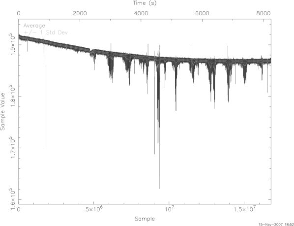
Figure 2.— An observation of RX J0806.4$-$4123 severely affected by RFI. Shown is the flux density in arbitrary units versus the time (top axis) or sample number (bottom axis) for about 8000 s of a 4-h observation. The plot was made by dedispersing the data with DM$=0$ pc cm^-3 using the prepdata program from the PRESTO package. Gray lines represent the average and $\pm 1\sigma$ contours. Each of these quasi-periodic negative bursts consist of many shorter leaps.

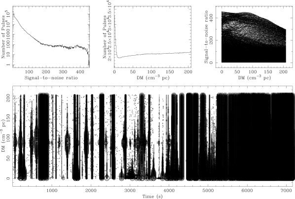
Figure 3.— The single-pulse search diagnostic plots for the 1.24-s pulsar J0628+09 without RFI excision (left) and with the manual RFI excision technique applied (using rfimarker, right). They have four smaller insets. Top: the histograms of the number of pulses versus S/N and DM, and the dependence of S/N versus DM (from left to right). Bottom: the main time-DM plot with the size of the points corresponding to the S/N of the pulse. The detection threshold is $5\sigma$. Vertical lines of pulses are either stronger at zero DM or roughly constant over all the DM range. They are RFI signatures rather than a real pulse, which would appear as a vertical segment of pulses with S/N peaking at a non-zero DM and gradually fading towards the edges of the segment (see bottom plot of the Fig. 4 how the pulse signatures appear for the low-DM fake pulsar). The train of pulses is clearly seen in the right plot (bottom inset). The strong peak in S/N-DM inset confirms the detection.

3.1. RFI Excision

For the half of the data that were not excluded, we created a mask to zap the RFI by using the rfifind package from PRESTO. Zapped samples were substituted by the mean of 80% of samples (excluding outliers) in every 30 s long chunk of data in each channel. However, even after applying the mask, the time series at dispersion measure $\mathrm{DM}=0$ pc cm^-3 and at larger values exhibited large outliers, fluctuations and jumps in the baseline levels. This is because rfifind deals only with strong broad-band outbursts by clipping them at $\mathrm{DM}=0$ pc cm^-3 (all spikes stronger than $6\sigma$ by default) and with periodic RFI (Scott Ransom, private communication). However, there were still many interference signatures left in the data of mostly non-periodic nature. In addition, some data were influenced by jumps in the baseline that could not be corrected by rfifind.

First, to overcome the jumps in power levels we divided the corresponding data into several sections and processed them separately. The fourth column in Table 1 shows the number of sections that were used for every observation. The duration of each observation is given in Table 2 (column 5). Then, we dedispersed every piece with $\mathrm{DM}=0$ pc cm^-3 and inspected these time series for RFI. To do this the rfimarker program was written. All records were inspected manually, and RFI-affected samples were selected by eye and flagged using a cursor. Then another program rficut read both the input data file and RFI binary list produced by rfimarker and replaced the bad samples by the average in a window of 131072 samples, excluding the top 10% of outliers. We also inspected the bandpass and if there were some frequency channels strongly affected by RFI, they were excluded from further analysis. This was done by providing a list of channels to ignore as an input option to the dedisperse program from the SIGPROC package. The percentage of channels that were ignored is listed in Table 2 (column 6). The advantage of RFI excision is shown in Fig. 3 where the diagnostic plot for the single-pulse search for pulsar J0628+09 is shown both for original data and the data with the masked RFI processed with rfimarker.

A careful reader may notice that in our paper we are focusing on searching for low-DM signals expected from nearby XDINSs rather than higher DM signals such as pulsar J0628+09. In the case of a low-DM source, the chance of occasionally zapping a real pulse from an XDINS is higher. Furthermore, in plots similar to Fig. 3, it would be more difficult to distinguish real pulses from zero-DM RFI. This is why the visual inspection aspect of rfimarker is important; much of the RFI has repeatable characteristic signatures that the trained eye will recognize. To show that rfimarker does not zap real pulses, we injected a fake pulsar signal into the real data shown in Fig. 3 contaminated by RFI. We cleaned these data with rfimarker, processed it in a range of DMs and made a diagnostic single-pulse plot. We chose a subset of data severely affected by RFI, namely a series of 600 s duration starting roughly 6000 s from the beginning of the observation (see Fig. 3). The range of DMs processed was 0–20 pc cm^-3; therefore the contribution from the pulsar J0628+09 itself, with DM$=88$ pc cm^-3, is negligible. The parameters of the fake pulsar were randomly generated from the range of the values we might expect for XDINSs, namely $P$ from 5–10 s, DM from 3–10 pc cm^-3, duty cycle from 0.1–2%, null fraction from 50–90% and peak SNR from 7–15. The results are shown in Figure 4. Without RFI excision, one can see many RFI peaks across the entire range of DMs with a larger contribution at lower DMs as expected. With RFI zapping, the plot looks cleaner, but one still can see several vertical lines similar to those we expected from RFI. They are, however, actually the pulses of the injected fake pulsar. After the injection of the fake pulsar and clipping we checked the parameters of the injected pulsar and how many pulses were injected (we did not know them in advance). There were 17 of them, in agreement with the null fraction for this fake pulsar, its period and data length. The number of these vertical lines is the same. The time differences between them all are equal to the integer number of periods of the fake pulsar (we used this technique for real XDINSs data, see Section 4.3). We did this experiment for several fake injected pulsars, with similar results. Therefore, this confirms that our manual RFI clipping technique does not zap real pulses.

However, as was mentioned above, it is difficult to distinguish between real low-DM pulses and RFI on the single-pulse diagnostic plots. This is because it is hard to tell whether the S/N peaks at a low DM or zero DM. Using Eq. 12 from Cordes & McLaughlin (2003), the ratio of the measured S/N of the pulse, when dedispersed with the wrong DM, to the true S/N, is almost 1 for a pulse width of 10 ms and error in DM of $1$ pc cm^-3 (given the observing frequency and total bandwidth of our observations). For a larger error in DM of $10$ pc cm^-3, this ratio is only 0.88 for a 10-ms pulse, and closer to 1 for broader pulses which we might expect from XDINSs. In any case, the broadening due to dispersion conserves the pulse area, and due to the matched filtering techniques we would get almost the same S/N, but with a larger effective sampling time, equal to the observed width of the pulse. Thus, there is no significant decrease in S/N for low-DM signals when one inspects the single-pulse diagnostic plots. All of the above considerations are true for high-DM pulsars as well, but in the diagnostic plots we inspect a much larger range of DM for them where the decrease in S/N at zero DM is more noticeable.

To combat this difficulty, we used the same technique which was used by McLaughlin et al. (2006) and resulted in the discovery of the rotating radio transients. The results of this search is given below in the Section 4.3.

Figure 4.— The time-DM plots from the single-pulse search analysis for the fake pulsar signal injected into real data without RFI excision (top) and with the RFI clipping technique applied (bottom). The RFI excision technique is described in Section 3.1. These plots are similar to the bottom insets of Fig. 3. Three other similar insets do not provide any necessary information and are not presented here. The real data used to inject the fake pulsar signal is the chunk of length 600 s from the observation of pulsar J0628+09 offset by 6000 s from the start of the observation (see Fig. 3). This particular chunk was greatly affected by RFI. The range of DMs processed is 0–20 pc cm^-3, thus the contribution from the pulsar J0628+09 with DM$=88$ pc cm^-3 is negligible. The parameters of the injected fake pulsar are: $P=7510.686$ ms, DM$=3.27$ pc cm^-3, duty cycle $=0.315$%, peak S/N $=10.3$, and null fraction = 79%. The vertical lines of large circles are true fake pulses rather than RFI.

3.2. Search pipeline

After the excision of RFI, each corrected observation was dedispersed for a number of different dispersion measures, DMs, from zero to a maximum value DM_max (column 7, Table 2) with a step size of roughly 1 pc cm^-3 (column 8). The DM spacing was determined by considering the dispersion smearing of $491.52~{}\mu$s (1 sample) in one frequency channel and the minimum pulse width of 1 ms. We chose the maximum value DM_max as double the prediction from the NE2001 model of free electron density in our Galaxy (Cordes & Lazio, 2002) assuming distances up to 1 kpc for all sources. The corresponding searched distance ranges are certainly much larger than any distance estimates for XDINSs (Posselt et al., 2007) or known parallax distances reported by van Kerkwijk & Kaplan (2007) and Kaplan et al. (2007). Once the data were dedispersed they were then searched for single pulses using the single-pulse search technique described in Cordes & McLaughlin (2003). The data were searched for periodic emission as well using two search techniques, the FFT and the FFA. Both single-pulse and FFT searches are incorporated in the SIGPROC pulsar software package. We wrote an FFA search code ffasearch to implement the FFA algorithm (see Appendix). This code has been proven to detect known long-period pulsars with higher signal-to-noise ratios (S/N) than traditional FFT searches.

Table 3XDINSs Results

	Pulsed emission			Bursty emission
XDINS	$S_{\mathrm{lim}}$	$L_{1400}^{\mathrm{p,max}}$	$L_{820}^{\mathrm{p,max}}$	rate upper limit	$S_{\mathrm{lim}}^{\mathrm{sp}}$	$L_{1400}^{\mathrm{b,max}}$
	($\mu$Jy)	(mJy kpc2)	(mJy kpc2)	(hr-1)	(mJy)	(mJy kpc2)
RX J0720.4$-$3125	$8$	$4\times 10^{-4}$	$10^{-3}$	$0.25$	$21$	$1$
RX J0806.4$-$4123	$10$	$4\times 10^{-3}$	$10^{-2}$	$0.32$	$18$	$6.9$
RX J1308.6+2127	$10$	$4\times 10^{-3}$	$10^{-2}$	$0.24$	$17$	$6.5$
RX J1605.3+3249	$8$	$3\times 10^{-3}$	$8\times 10^{-3}$	$0.25$	$22$	$8.4$
RX J1856.5$-$3754	$14$	$1.4\times 10^{-4}$	$3.6\times 10^{-4}$	$0.32$	$24$	$0.2$
RX J2143.0+0654	$13$	$5\times 10^{-3}$	$1.3\times 10^{-2}$	$0.36$	$20$	$7.6$

4. Results

No pulsed radio emission or isolated pulses were found from any of the six observed isolated neutron stars. Table 3 summarizes the results. Column 1 lists the name of the source, column 2 gives the $4\sigma$ flux upper limits $S_{\mathrm{lim}}$ on pulsed radio emission for an assumed pulse duty cycle of 2%, and column 3 lists the upper limit on radio luminosity at 1400 MHz, $L_{1400}^{\mathrm{p,max}}$, in mJy kpc² assuming spectral index $\alpha=-1.8$ and either measured parallax distances from Table 2 (column 4) for two XDINSs or a very conservative distance estimate of 1 kpc. Column 4 gives the radio luminosity at our observing frequency of 820 MHz, $L_{820}^{\mathrm{p,max}}$, with the same distance assumptions as for column 3. Columns 5–7 summarize the results on single-pulse emission and list the upper limits on single-pulse detection rate, peak fluxes $S_{\mathrm{lim}}^{\mathrm{sp}}$ and radio luminosities $L_{1400}^{\mathrm{b,max}}$ with the same assumptions as for radio luminosity for pulsed emission. The spectral indices of XDINSs are unknown, and for our estimates we used the mean value of $-1.8$ measured for known radio pulsars (Maron et al., 2000).

4.1. FFT Search

Though the FFT search is not efficient for long period sources (see A.3), we still applied it to every observed XDINS. We tried three incoherent harmonic summations with 32, 64, and 128 harmonics. However, we did not find any promising candidates.

4.2. FFA search

On the contrary, the FFA search should be very effective for long-period pulsars. The ffasearch program was written to implement the FFA algorithm (see Appendix). We performed this search for period ranges within 200 ms of the reported X-ray period (see Table 2). These ranges are much larger than the difference between the reported barycentric X-ray period value and the topocentric period at the date of observation even for a period derivative as large as $\dot{P}=10^{-11}$ s s^-1. They are also much larger than any reasonable uncertainties in the X-ray periods. Following the matched filtering technique by Cordes & McLaughlin (2003), every profile was rebinned by different factors from 1 (no rebinning; sampling interval is $491.52~{}\mu$s) to $N$, where $N$ corresponded to a sampling interval approximately equal to 0.04$P$, where $P$ is the X-ray period. Thus, our search was sensitive for all possible pulse widths up to duty cycles of 4%. We have inspected the folded profiles for many candidates and did not find any significant profiles down to a $4\sigma$ detection threshold. Those profiles with peak fluxes still above a $4\sigma$ level were undoubtedly of RFI nature because they were detected over a broad range of DMs including $\mathrm{DM}=0$ pc cm^-3. We therefore quote a $4\sigma$ upper limit on pulsed radio emission. As an example, Fig. 5 shows an FFA diagnostic plot for RX J0720.4$-$3125. The presence of a real pulsed source would show up as an elongated train of candidates in both period and DM axes.

Figure 5.— Example of an FFA diagnostic plot for RX J0720.4$-$3125. The top-left plot is the periodogram, i.e. the folded profile’s significance for every periodic candidate, the top-right plot shows the profile significance versus DM. The plot on the bottom represents the S/N of the folded profiles versus DM and the period. The darker points have larger S/Ns. The expected signature of the pulsar is a bar of increased flux along the DM axis (see Appendix for more details). Long lines over a broad DM range are not real but rather due to strong RFI of periodic origin.

4.3. Single-Pulse Search

The single-pulse search is a very powerful tool to detect strong individual pulses from sources whose regular, periodic emission is too weak to be detected through a periodicity search. The RRATs were discovered in this way (McLaughlin et al., 2006). XDINSs show possible connections with the RRATs, thus making the single-pulse search very important.

We performed a single-pulse search for each isolated neutron star in our analysis. The search was done for a range of pulse widths using the matched filtering technique (Cordes & McLaughlin, 2003) up to maximum widths of about 503 ms (ten consecutive summations of neighboring samples). If pulses were detected with several different matched filters, only the candidate with the largest S/N was recorded. For every XDINS we obtained the candidates list of all events stronger than $5\sigma$ and single-pulse diagnostic plots similar to those in Fig. 3, 4. However, as was discussed in the Section 3.1 it is very hard to distinguish real low-DM signals from zero-DM RFI in these plots.

To overcome this difficulty, we can make use of the fact that any pulses from an XDINS should be emitted modulo the known rotation period (see Table 2). By searching for the greatest common denominator of the differences between all of the pulses, we can determine whether they have an underlying periodicity. This was the method used to reveal the periods of the rotating radio transients (McLaughlin et al., 2006). Due to the inevitable presence of some pulses due to RFI, we simply report the period that fits the greatest number of differences, but do not require that all pulses fit. We applied this method to the test pulsar J0628+09 and the fake pulsar from Fig. 4. For the pulsar J0628+09 we found that, despite the presence of pulses due to RFI, the underlying pulsar periodicity was evident. The fake pulsar periodicity was found in the clipped data only, emphasizing the importance of the RFI mitigation. Applying this method to the single pulses detected in this XDINS search revealed no obvious periodicities. Because we know the periods of the XDINSs a priori, we also performed another search in which we took all of the differences between pulses and divided by the known period. There was no evidence that any of the differences between detected pulses were integer multiples of the spin period.

We therefore can conclude with confidence that our single pulse search did not detect any pulses from the XDINSs.

4.4. Flux Upper Limits

The minimum detectable flux of our survey strongly depends on the pulse duty cycle, $\delta$, as

$$S_{\mathrm{lim}}=354\frac{T_{\mathrm{sys}}\cdot\mathrm{S/N}}{\sqrt{t_{\mathrm{run}}~{}\!B}}\sqrt{\frac{\delta}{1-\delta}}~{}\mu\mathrm{Jy}$$ (1)

for our observing setup at 820 MHz. In this expression, $T_{\mathrm{sys}}$ is the system temperature in K including sky contribution, $t_{\mathrm{run}}$ the observing time in seconds, $B$ the effective bandwidth in MHz, and S/N the detection threshold. Assuming a reasonable value of $\delta=2\%$, greater than the duty cycle of 65% of pulsars with $P>2$ s, our $4\sigma$ detection limits range from 8 to $14~{}\mu$Jy for different XDINSs depending on the length of the observation and number of ignored frequency channels, i.e. the effective bandwidth. The list of the flux upper limits is given in Table 3 (column 2). The single-pulse duty cycles of the RRATs are even smaller than 2%, with the mean value around 0.5% (McLaughlin et al., 2006; McLaughlin, 2009a). If the integrated duty cycles of possible radio emission from XDINSs are the same as for RRATs, then the flux limits are even smaller than those listed.

For single radio pulses, the flux limits can be obtained from

$$S_{\mathrm{lim}}^{\mathrm{sp}}=11.2\frac{T_{\mathrm{sys}}\cdot\mathrm{S/N}}{\sqrt{w~{}\!B}}~{}\mathrm{mJy}~{},$$ (2)

where $w$ is the assumed pulsed width, and other quantities are the same as in equation (1). Assuming pulse widths $w=0.02P$, where $P$ is the X-ray period, we derive $5\sigma$ upper limits on single-pulse fluxes ranging from 17 to 24 mJy. This list is given in column 6 of Table 3. These limits are more than 5 times smaller than the peak fluxes of the strongest single pulses from the RRATs (McLaughlin et al., 2006; McLaughlin, 2009a). For two RRATs, J0848$-$43 and J1839$-$01, the peak fluxes of the strongest pulses are 100 mJy at 1400 MHz, which means that they should be even larger at our frequency of 820 MHz, assuming typical pulsar spectral indices. If XDINSs manifested the same single-pulse properties of the RRATs, they should be easily detected in our observations at about the $60\sigma$ level.

4.5. Test observations of known radio pulsars

We successfully applied the same search pipeline to data taken during the same observing session with the same observational setup on the 246-ms pulsar B0540+23, the relativistic binary pulsar B1534+12, and the 1.24-s pulsar J0628+09. They were detected with all three search methods (see, for instance, Figs. 3 and 7). For the pulsar J0628+09 the first FFT run did not detect the main pulsar harmonic using the default incoherent foldings of 32 harmonics. The subsequent runs with the summation of 64 and 128 harmonics found the pulsar at a frequency of 0.8055 Hz ($P=1241.477$ ms) with S/N $=17.2$ and $19.5$, respectively. The value of 128 summed harmonics corresponds roughly to the pulse width of about 10 ms ($N_{\mathrm{harm}}\sim P/w$). The S/N of the integrated profile with a bin width of 10 ms is consistent with the spectral S/N and is about 20. This corresponds to a mean flux density of about $40~{}\mu$Jy at 820 MHz. Note that this pulsar was originally detected only through a single-pulse search (Cordes et al., 2006). For the relativistic binary B1534+12 the FFT and FFA searches give S/Ns of about 11 and 8, respectively. Including an acceleration search increases the S/N to 30, corresponding to a mean flux of about 0.35 mJy. This value is smaller than the expected mean flux at our observing frequency of about 3.4 mJy (Wolszczan, 1991; Kramer et al., 1998) and can be accounted for by scintillation. The pulsar B0540+23 was found with S/N of 76 in the FFT search with 32 harmonics folds and of about 240 in the FFA search. The mean flux of about 7 mJy that corresponds to S/N = 240 is about 3 times less than the expected flux at this frequency. This can be due to interstellar scintillations with a timescale of about several minutes (observing time was only 1 min). System overflow could also have been an issue because the pulsar is very strong, and the inherent 3-level sampling of the SPIGOT is subject to saturation for bright sources. The presence of artifacts in the average profile further supports this suggestion.

5. Discussion

The elusive radio emission of XDINSs, the sporadic radio activity of the RRATs, and the recently discovered transient radio emission from allegedly ‘radio-quiet” magnetars (Camilo et al., 2006, 2007) hint at close relationships between these classes of neutron stars. Popov et al. (2006b) have shown that the implied birthrate of RRATs is more consistent with that of XDINSs than that of magnetars. As shown in the $P$-$\dot{P}$ diagram (Fig. 1), RRATs and XDINSs also have similar periods and period derivatives, implied ages and magnetic fields. Moreover, X-ray observations of one RRAT (McLaughlin et al., 2007) reveal properties similar to those of XDINSs (i.e. a purely thermal spectrum with $kT\sim 140$ eV and a broad absorption feature at $\sim 1$ keV). However, the RRATs spin-down properties are also consistent with those of the normal pulsar population and transient magnetars in quiescence. The nearby ($\simeq 300$ pc) radio pulsar B0656+14, in addition to underlying weak emission of broad pulses, manifests extremely bright spiky emission (Weltevrede et al., 2006). Because of this, it would only be detected as an RRAT were it placed at a distance of a few kiloparsecs (Weltevrede et al., 2007).

The distances to the XDINSs are also believed to be much smaller than those to the RRATs ($\lesssim 1$ kpc). Thus, we should have had high sensitivity to RRAT-like radio emission. Indeed, with the average $1\sigma$ sensitivity to single radio pulses of 4 mJy for the XDINSs, the strongest pulses, with the same properties as those of the RRATs (McLaughlin, 2009a), would be detected with S/N $>60$. However, we have not detected such isolated radio pulses or any periodic emission from the six XDINSs we have observed. Our non-detection of such emission, however, does not necessarily mean that there is no relationship between the two source classes.

The radio emission of XDINSs may simply be more sporadic than that of the RRATs. We estimated the upper limits on the rates of possible pulses from the XDINSs as less than one event in the full observing time for every source (see Table 3, column 5). These limiting pulse rates range from 0.24 pulses per hour for RX J1308.6+2127 to the maximum rate of 0.36 for RX J2143.0+0654. The smallest average pulse detection rate of the known RRATs is 0.3 pulses per hour for J1911+00. This value corresponds exactly to the average upper limit on pulse detection rates for all XDINSs. However, some RRATs, like J1839–01, show extreme variations in their pulse detection rates and have periods where the detection rate is much less than 0.3 pulses per hour.

Another possibility is that XDINSs may be truly “radio-weak” or “radio-quiet”. The derived upper limits for the radio luminosities of pulsed emission at 1400 MHz $L_{1400}^{\mathrm{p,max}}$ are very small, $(0.14-5)\times 10^{-3}$ mJy kpc² (Table 3, column 3). No normal radio pulsars are known to have such low values of radio luminosity at 1400 MHz, with only six radio pulsars having values smaller than 0.1 mJy kpc². However, this could be due to our lack of knowledge about the spectral indices of XDINSs. In our estimates we have used the mean value of spectral indices for normal radio pulsars of $-1.8$. To avoid using such an uncertain quantity we also compared radio luminosities of XDINSs with that of normal radio pulsars at our frequency of 820 MHz. Upper limits of the radio luminosities of XDINSs at 820 MHz are listed in column 4 of Table 3. For comparison we chose 285 pulsars with known spectral indices and radio luminosities at either 1400 or 400 MHz. The lowest derived value of radio luminosity at 820 MHz is 0.17 mJy kpc² for PSR J0030+0451 with only 8 pulsars having luminosities below 1 mJy kpc². Thus, by any means the pulsed radio luminosities of XDINSs are much weaker than those of normal radio pulsars. Column 7 of Table 3 lists the upper limits for single-pulse luminosity at 1400 MHz. They are all less than 10 mJy kpc², but probably the true value is even less, $<1$ mJy kpc², as for RX J0720.4$-$3125 and RX J1856.5$-$3754 with measured parallax distances. The minimum single-pulse luminosities for RRATs are believed to be about 100 mJy kpc² (McLaughlin et al., 2006; McLaughlin, 2009a). Therefore, the “radio-weak” or “radio-quiet” scenario is consistent with our results.

Perhaps the most likely possibility, however, is that XDINSs simply represent a sub-sample of long-period ordinary radio pulsars with relatively high magnetic fields. Being nearby objects, their radio emission could escape detection in our deep observations due to unfavorably aligned radio beams. Indeed, assuming the radio pulsar mean beaming fraction $f=0.1$ (Tauris & Manchester, 1998), i.e. the probability that any pulsar’s emission beam intersects our line of sight, then the probability that all six XDINSs are beamed away from the Earth is $(1-f)^{6}=53\%$. For long-period pulsars this probability could be even as high as $83\%$, if instead of the mean value of $0.1$ one uses the relation (15) from Tauris & Manchester (1998) between beaming fraction and the pulsar period, for the periods from Table 2. In other words, we would need a sample of about 40 sources to provide a $1\sigma$ probability of at least one of their radio beams intersecting our line of sight.

Are there any long-period high-$B$ normal radio pulsars known to emit in X-rays, and if so, are their properties consistent with those of XDINSs? There are 34 rotation-powered radio pulsars in our Galaxy, listed in the ATNF pulsar catalog, with periods $>1$ s and magnetic fields $B>10^{13}$ G. As discussed, the X-ray properties of RRAT J1819$-$1458 are remarkably similar to those of XDINSs (McLaughlin et al., 2007). To our knowledge only four of the remaining 33 — B0154+61, J1718$-$3718, J1814$-$1744 and J1847$-$0130  — have been observed in X-rays. No X-ray emission was detected from the $B=2.1\times 10^{13}$ G, $P$ = 2.3 s PSR B0154+61 in a 31-ks observation with XMM-Newton (Gonzalez et al., 2004). Archival ROSAT and ASCA data (duration of 7.7 and $2\times 11.5$ ks, respectively) do not reveal X-ray emission from the field of the $B=5.5\times 10^{13}$ G, $P$ = 3.9 s PSR J1814$-$1744 (Pivovaroff et al., 2000). A recent 6-ks observation with Chandra also resulted in a non-detection (PI: Camilo, proposal number 0207010101). No X-ray emission was also found from the 6-ks ASCA archival data of the field containing J1847$-$0130, with $B=9.4\times 10^{13}$ and $P$ = 6.7 s. (McLaughlin et al., 2003). However, for pulsar J1718$-$3718, with $B=7.4\times 10^{13}$ G and $P$ = 3.3 s, very faint X-ray emission was found by Kaspi & McLaughlin (2005) in a much longer 55.7-ks Chandra observation. The thermal spectrum resembles that from XDINSs, but a longer observation of J1718–3718 is needed to draw any firm conclusions.

While B0154+61 has a DM-derived distance of only 1.6 kpc, the non-detection of X-ray emission from the very high magnetic field pulsars J1847–0130 and J1814–1744 could be due to their large distances (7.7 kpc and 9.8 kpc, respectively, compared with 4.9 kpc for X-ray faint J1718$-$3718) and the shorter integration times used. If deeper X-ray observations would allow to detect and recognize them as XDINSs, this will strongly support the hypothesis that XDINSs are simply nearby long-period high-$B$ normal radio pulsars beamed away from us. Rapidly evolving to long periods, they still can be detected in X-rays if they are nearby and cooling of the neutron star is not yet completed. Further X-ray and optical observations with long integration times of long-period high-$B$ radio pulsars are necessary to confirm their relation with XDINSs.

This attractive picture, however, does not agree well with the results from population syntheses. Under the standard assumptions about neutron star cooling (see Page et al., 2006,  and references therein) the birth rate of XDINSs is higher than that of high-$B$ pulsars (Popov et al., 2006b; Vranesevic et al., 2004). The XDINSs can be older, and so have a lower birth rate consistent with that of long-period high-$B$ radio pulsars, only if their cooling does not follow the standard model (e.g., Blaschke et al., 2004; Page et al., 2004; Yakovlev & Pethick, 2004). This, however, is very improbable because standard population synthesis models reproduce the local population of neutron stars very well (e.g., Popov et al., 2006a). The assumption that the birth rate of high-$B$ pulsars is underestimated, though possible, does not correspond to the log-normal distribution of the magnetic fields of the pulsar population (Faucher-Giguere & Kaspi, 2007). A joint population synthesis of radio pulsars and cooling isolated neutron stars with non-standard assumptions — such as, heating due to magnetic field decay and influence of magnetic fields on cooling (Pons & Geppert, 2007; Aguilera et al., 2008) — could be very relevant. It is certainly possible that XDINSs represent a small group of sources with unique properties and narrow radio beams which do not intersect our line of sight.

Searches at lower frequencies, where radio emission beams are believed to be wider (Radhakrishnan & Cooke, 1969), may be more sensitive to radio emission from XDINSs. Indeed, Malofeev et al. (2005, 2007) reported the detection of radio emission from RX J1308.6+2127 and RX J2143.7+0654 at the low frequency of 111 MHz. If the detection of Malofeev and co-authors is real, our non-detection of radio emission from these two XDINSs at 820 MHz implies that their spectral index $\alpha<-4$.

In summary, we have presented the most sensitive limits so far on periodic and transient radio emission from XDINSs. The lack of detection makes comparisons between XDINSs and other radio populations of neutron stars difficult. It is possible that the radio emission from XDINS is truly very weak, but it is also quite plausible that XDINs have normal radio luminosities, but are simply beamed away from us. Observations at lower frequencies are necessary to further constrain the presence of any radio emission. Extensive high-energy studies (X-ray, optical) of known long-period high-$B$ normal radio pulsars and RRATs are required to support the hypothesis that they belong to the same group as XDINSs. The detection of more XDINSs and subsequent radio followup observations are also crucial in this regard.

Appendix A Fast Folding Algorithm

The Fast Folding Algorithm (FFA) was originally developed by Staelin (1969) to detect periodic signals in noisy data. While the Fast Fourier Transform (FFT) accomplishes this task in the frequency domain, the FFA works in the time domain. The FFA is much faster than simply folding over a range of trial periods. The computational time is reduced by avoiding the redundant summations for many trial foldings for different periods. In this appendix we will not repeat the mathematical details of the algorithm, but will rather focus on specific aspects of applying this technique to pulsar searches. The necessary background on the FFA itself can be found both in the original paper by Staelin (1969) as well as in Lovelace et al. (1969), Burns & Clark (1969), Hankins & Rickett (1975), and Lorimer & Kramer (2004).

A.1. Description

We start with a time series of $N$ samples taken with sampling interval $\Delta t$ which contains a periodic signal too weak to be detected over the noise without folding. For pulsar searches, this would be a time series dedispersed at some particular dispersion measure, DM. A single FFA transaction calculates the number of trial folded profiles $M=N/P_{0}$ in the range from $P_{0}$ to $P_{0}+1$, where $P_{0}$ is the trial base period in samples. The trial base period in time units $P_{0}^{\mathrm{t}}$ is then $P_{0}^{\mathrm{t}}=P_{0}\times\Delta t$, and the period of every folded profile can be determined by

$$P^{\mathrm{t}}=\left[P_{0}+\frac{1}{M-1}i\right]\times\Delta t=P_{0}^{\mathrm{t}}+\frac{P_{0}^{\mathrm{t}}}{N-P_{0}}i~{},$$

where $0\leq i\leq(M-1)$. The step $\Delta P$ is determined by the integer number of periods in the time series and the sampling interval of the data, i.e. $\Delta P=\Delta t/(M-1)=(P_{0}\cdot\Delta t)/(N-P_{0})=P_{0}^{\mathrm{t}}/(N-P_{0})$. The only thing the FFA requires is for the ratio $M$ to be a power of 2, or $\log_{2}(N/P_{0})$ to be an integer. Another implementation of the original FFA by Lovelace et al. (1969) requires both $N$ and $P_{0}$ to be a power of 2 rather than just their ratio. Without the FFA this procedure would require $N^{2}/P_{0}$ summations, whereas with the FFA it is just $N\log_{2}(N/P_{0})$.

In practice, the usual period range to be searched can be as large as several seconds, or in some specific cases only a few milliseconds (for instance, when you know the period from observations at other wavelengths, as in the case of the XDINSs). The FFA search will typically result in higher signal-to-noise ratio than FFT for pulsars with periods $>6$ s and pulse duty cycles up to 4%, or even for pulsars with periods $\gtrsim 2$ s and small duty cycles up to 0.8% (see below). In the frequency domain, these long periods correspond to frequencies of 1 Hz and less, which are in the lower part of the spectrum, presumably dominated by red noise, making the FFT less efficient than the FFA.

A.2. Implementation

The described FFA method was implemented as a C program ffasearch to search for pulsars in noisy time series. It executes successive single-algorithm operations for different $P_{0}^{\mathrm{t}}$ from $P_{\mathrm{low}}$ to $P_{\mathrm{high}}$, the values of which are specified in the command line. As the result, the sifted and full lists of candidates are created together with a plot containing the periodogram and plots of the folded profiles for the three best candidates. An example of this diagnostic plot is shown in Fig. 6 for the 1.24-s pulsar B0628+09. Some details of the candidate selection procedure, the candidate sifting, rebinning, and duty cycles issues are given briefly below.

Figure 6.— FFA diagnostic plot for a 2-hr observation of the 1.24-s pulsar J0628+09. The top left plot represents the periodogram, i.e. the S/N of the most significant peak in the folded profile as a function of trial period. The three crosses in the plot mark the S/Ns of the three best candidates. The other three plots, top-right and from left to right on the bottom, are the folded profiles for those three best candidates. The profile of the best candidate (top-right) was folded with a trial period very close to the true topocentric period of pulsar J0628+09 and has a S/N of about 9. The matched filtering technique was applied with the rebinning of folded profiles by up to 4 samples ($983~{}\mu$s). The legend at the bottom shows the range of the searched periods and trial periods of the three best candidates together with some other information.

Candidate selection. For every base trial period $P_{0}$ we have $M$ different folded profiles with periods spaced by $\Delta P$. From them we select only the three best candidates with the highest signal-to-noise ratios (S/N) of the maximum peaks in their profiles, S/N = $(I_{\mathrm{max}}-\langle I\rangle)/\sigma$, where the average intensity $\langle I\rangle$ and rms $\sigma$ in the folded profile are calculated by excluding a window centered on the peak $I_{\mathrm{max}}$. The size of this window is 20% of the size of the profile. For every candidate, we save S/N, period, the phase of the maximum, the number of other candidates with smaller S/Ns with the same phases of the three best candidates, and duty cycle (see below). The full list of all detected candidates is recorded into an ASCII file with other information such as DM, sampling interval, etc.

Sifting. Even with only three candidates for every trial base period $P_{0}$, the final output list is very large, with many candidates having similar periods. We therefore sift the full list, sorting by S/N and excluding candidates with periods within 3% of the period of any of already sifted candidates. In the sifted list for every candidate the number of other candidates with close periods that were excluded is noted.

Rebinning. Often the sampling interval of the time series is very small in comparison with the expected pulse width of a pulsar. Therefore, rebinning will help to increase the S/N and speed up the search process. There are three different types of rebinning that were implemented: (a) the preliminary decimation of the time series by several samples before starting the FFA; (b) rebinning of each of $M$ trial periods $P_{0}$ before starting the FFA search; (c) extra rebinning of every trial folded profile after the FFA run. Both (a) and (b) decrease the time resolution of the original time series, increase $\Delta P$ and decrease the execution time. However, the “b”-rebinning has the major advantage over the “a”-decimation that for every trial $P_{0}^{\mathrm{t}}$, all $M$ periods are summed in phase, thus increasing the S/N of pulsar candidates (the “a”-decimation and “b”-rebinning are the same only when $P_{0}$ is an integer multiple of the decimation factor, which is very unlikely). The extra “c”-rebinning represents the matched filtering technique described by Cordes & McLaughlin (2003) for every folded profile after FFA run and was implemented to be sensitive for pulsars with different pulse widths. This rebinning will not decrease the period resolution $\Delta P$ and is a small increase in the execution time in comparison with the time required to run through all FFA operations. For long time series, it is typically necessary to use the preliminary decimation to fit the entire data segment into memory, and then use the “b”-rebinning to ensure reasonable execution times.

It is important to distinguish between rebinnings (b) and (c). The latter is applied to each of $M$ trial folded profiles for periods between $P_{0}^{\mathrm{t}}$ and $P_{0}^{\mathrm{t}}+\Delta t$ after the FFA. This procedure is the one that was referred to by Lovelace et al. (1969) as searching different pulse widths “by adding the sums corresponding to different phases”. The “b”-rebinning is applied not to trial folded profiles but to each of $M$ periods $P_{0}$ before the FFA run. This has the advantage of significantly decreasing the number of FFA summations and the FFA execution time by reducing the number of bins in the final folded profiles (if there is no need for smaller time resolution).

Duty cycles. The choice of rebinning determines the duty cycles of the pulsars to which the FFA is most sensitive. Owing to the definition of S/N based on the single maximum bin in the folded profile, optimal detection will occur when the pulse width is similar to the final sampling interval. Therefore, one should consider the overall preliminary decimation and rebinning within the FFA as the one that determines the minimal pulse width (or duty cycle) optimized in this particular search. Thus, if one searches the data from $P_{\mathrm{low}}$ to $P_{\mathrm{high}}$ with an interval between adjacent bins of $\Delta t_{\mathrm{ffa}}$ then duty cycles ranging from $\Delta t_{\mathrm{ffa}}/P_{\mathrm{high}}$ to $\Delta t_{\mathrm{ffa}}/P_{\mathrm{low}}$ are covered optimally. However, to increase the sensitivity of the search to pulsars with larger duty cycles, it is worthwhile to rebin all the folded profiles by different factors covering a larger range of duty cycles (i.e. the matched filtering technique, see Cordes & McLaughlin, 2003). The ffasearch program is now implemented in a way to perform this matched filtering (or “c”-rebinning) of folded profiles after the FFA run for a selected range of pulse widths with an increment of 1 bin.

In addition to implementation of the FFA itself, a Perl-script, ffadmplot, was written that combines the FFA results for all trial values of DM in a number of diagnostic plots. An example of this plot for pulsar J0628+09 is shown in Fig. 7. At the bottom is a DM-$P$ gray-scale plot with darker points corresponding to candidates with higher S/Ns. The other two plots on the top show S/N as a function of trial period and DM. For the bottom plot, one can use either grayscale or circles such as used for the single-pulse diagnostic plots. This script has interactive plotting, allowing the user to examine every point in all of three plots, select the candidates, and make a plot with folded profile for every selected profile. As shown in Fig. 7 the true pulsar period is clearly seen in the bottom plot.

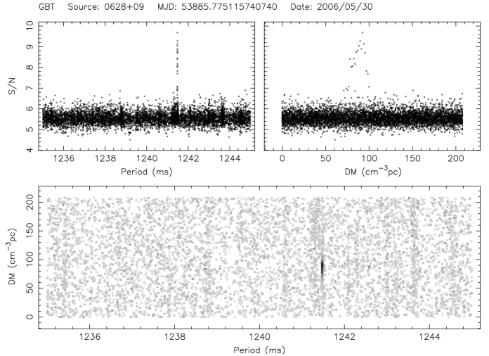
Figure 7.— An FFA diagnostic plot combining the results for a range of trial DM values for the 1.24-s pulsar J0628+09. The bottom plot represents DM-$P$, with darker points corresponding to candidates with higher S/N. The two top plots are S/N of the candidates as a function of a trial period $P$ (top-left) and trial DM (top-right). The actual pulsar values of period and dispersion measure are clearly seen in all three plots.

A.3. FFA vs. FFT

Simulation. To compare the efficiency of both the FFA and the FFT, we performed FFA and FFT searches on artificial pulsar signals with different periods and pulse widths. For this purpose we used the fake program from the SIGPROC package. This program creates time series of Gaussian noise with injected top-hat pulses with predetermined period, width and peak signal-to-noise ratio. Then we ran both FFT and FFA searches on these time series with the fake pulsar, recording the S/N with which the pulsar was detected in both searches. The sampling interval was chosen to be $491.52~{}\mu$s, the same as in the real XDINS data. The number of generated samples corresponded to an observing time of 1 hour. The simulation was done for pulsar periods, $P$, ranging from 2 to 14 s with a step of 0.5 s and for 14 different values of pulse duty cycle, $\delta$, covering $0.1-1$% (with stepsize 0.1%) and $2-5$% (with stepsize 1%). Therefore, in total we have 350 fake pulsars with different $P$ and $\delta$. The peak fluxes of injected top-hat pulses were different for different $P$ and $\delta$ to keep the total pulse energy the same among all trial fake pulsars. Thus, the peak flux density was less for broader pulses. The number of harmonics summed in the FFT search was 32. For every combination of $P$ and $\delta$ we performed 30 different trials recording the S/Ns from both searches. The results of our simulations are shown on Fig. 8 (left, dots) for two cases of $\delta=0.2$ and $1\%$. For other duty cycles the obtained dependencies are similar.

The plots show the dependence of the S/N for both FFT and FFA searches as a function of period. In addition to the results from the simulation, the lines represent the derived analytical dependence (see below). The apparent decrease of the S/Ns with increasing period and duty cycles is due to our requirement of constant energy for all individual pulses, and because of fewer numbers of larger periods in our fixed observing time. It is clearly seen that for smaller duty cycles (0.2%, narrower profiles) the FFA search performs better than the FFT even for small periods. However, this is not that relevant as most pulsars with duty cycles $<1$% have long periods. For instance, of 25 radio pulsars in the ATNF catalog with duty cycles $<0.8$%, 19 have period $>1$ s. The broader the pulse (the larger $\delta$), the longer the pulsar period should be in order for the FFA search to be more efficient than the FFT search, particularly for the $\delta=1\%$ the FFA search is only more efficient than FFT search for periods more than 4 s. It is worth mentioning that fake pulsars with periods $>10$ s and large duty cycles of 2–5% were not detected in the FFT search in every trial. This demonstrates the importance of using an FFA search for very long period pulsars.

Analytic approach. In addition to the simulation, we can also make a comparison between the FFA and FFT effectiveness from analytical considerations. Our simulation showed that the FFA is advantageous for pulsars with short duty cycles. This is because short duty cycle pulsars distribute their power over many harmonics, and only a limited number of harmonics are summed together in the FFT search. This number depends on the particular FFT search procedure used, but a typical maximum number of summed harmonics is 32 (as in the current search and simulation). Moreover, these harmonics are summed incoherently, further reducing the S/N that can be achieved with the FFT. Contrary to the FFT search, the FFA search folds all the data in phase, or coherently. Larger S/Ns can also be reached for pulsars with larger duty cycles (broader pulses) by rebinning the profiles with an optimal window equal to pulse width. Thus, assuming that no power is lost in the FFA search, and estimating the power that can be recovered during an incoherent sum of a finite number of harmonics for the FFT search, we can derive an analytical expression for the ratio of detected S/Ns for the FFA and FFT search for a particular pulsar.

Consider for simplicity the periodic train $\Pi(t)$ of top-hat pulses with amplitude $S$, period $P$, and pulse width $w$ in the presence of noise $n(t)$ with zero mean and standard deviation of unity. We can write the pulse amplitude $S$ as $E_{p}/\delta P$, where $\delta=w/P$ is the pulse duty cycle, and $E_{p}=wS$ is the pulse energy, chosen to be constant for all artificial pulsars in our simulations described above. The signal-to-noise ratio, $(\mathrm{S/N})_{\mathrm{ffa}}$, of the single pulse in a non-decimated time series $\Pi(t)+n(t)$ is then equal to its amplitude $S$. By folding all periods together we increase the $(\mathrm{S/N})_{\mathrm{ffa}}$ by $\sqrt{N_{p}}$, where $N_{p}=N/P=T/P^{t}$ is the total number of periods in the time series, $N$ the total number of samples, $T=N\Delta t$ the observing time (1 hour in our simulation), $\Delta t$ the sampling interval ($491.52~{}\mu$s in the simulation) and $P$ or $P^{t}$ the pulsar period either in samples or time units. One can also increase the $(\mathrm{S/N})_{\mathrm{ffa}}$ by using the matched filtering technique, i.e. by rebinning the folded profile with the optimal window of pulse width $w$. This will increase $(\mathrm{S/N})_{\mathrm{ffa}}$ by $\sqrt{w}$. Thus, finally, the signal-to-noise ratio of our pulse train $\Pi(t)$ from the FFA search becomes

$$(\mathrm{S/N})_{\mathrm{ffa}}=\frac{E_{p}\sqrt{N}}{P^{t}\sqrt{\delta}}~{}.$$

To obtain the corresponding signal-to-noise ratio of the FFT-search $(\mathrm{S/N})_{\mathrm{fft}}$, we derive first the Fourier response of our pulse train $\Pi(t)=\sum_{l=0}^{\infty}S\Pi\left[(t-lP+P/2)/w\right]$, where $\Pi(t)$ represents the rectangular top-hat function of width and height equal to unity. The term $P/2$ reflects the shift by half of the period from the origin (as in our simulated pulse trains). It is easy to show that the complex $n$-th Fourier harmonic $F_{n}$ of this pulse train $\Pi(t)$ is given then by $F_{n}=-2S(1-\delta)\mathrm{sinc}[\pi n(1-\delta)]$ (see, e.g., Bracewell, 2000). The response of the discrete Fourier transform (DFT) $A_{k}$ in the FFT search for $n$-th harmonic is $NF_{n}/2$ for the ideal case when the frequency of the harmonic coincides exactly with the frequency of the corresponding Fourier bin $k$, i.e. $nN/P=k$, $k=0,1,\ldots,N-1$. Usually this is not the case and the harmonic amplitudes will be reduced by a factor of $\mathrm{sinc}[\pi(k-nr)]$, where $r$ is the real wavenumber defined as $r=N/P$ (so-called “scalloping” effect; see, e.g., Ransom et al., 2002). However, in our FFT search the interbinning technique was used that improves the DFT response with a loss of sensitivity of not more than $\sim 7.4\%$. Therefore, in our further consideration we will only consider the case without scalloping.

To estimate the average response of our harmonics in presence of noise and convert it into the S/N units we need to know what are the values of the mean and root-mean-square deviation in our amplitide spectrum $A_{k}=[{(c_{k}+a^{\prime}_{k})^{2}+(d_{k}+b^{\prime}_{k})^{2}}]^{1/2}$, where $c_{k}$ and $d_{k}$ are real and imaginary parts of the spectrum related to the signal, and $a^{\prime}_{k}$ and $b^{\prime}_{k}$ are real and imaginary parts of the spectrum related to noise. The $a^{\prime}_{k}$ and $b^{\prime}_{k}$ are independent and normally distributed with the mean zero and variance of $N/2$. The normalized amplitude spectrum of such a kind obeys the non-central $\chi$-distribution with two degrees of freedom (Evans et al., 2000; Johnson et al., 1994), and characteristic parameter ${\lambda}_{k}=[(2/N)\cdot(c_{k}^{2}+d_{k}^{2})]^{1/2}$, where $c_{k}^{2}+d_{k}^{2}=N^{2}F_{n}^{2}/4$ for all $k=N/P,2N/P,\ldots$ and zero otherwise. The mean, $\mu_{k}$ and rms, $\sigma_{k}$ of this distribution are defined as $\mu_{k}=(\pi/2)^{1/2}\cdot L^{0}_{1/2}(-\lambda_{k}^{2}/2)$ and $\sigma_{k}=(2+\lambda_{k}^{2}-\mu_{k}^{2})^{1/2}$, where $L^{0}_{1/2}(x)$ is the generalized Laguerre polynomial $L^{(\alpha)}_{n}(x)$ of degree $n=1/2$ and $\alpha=0$. Hence, every Fourier bin of our spectrum will have its own mean and rms values. For the harmonics related to our periodic signal $\Pi(t)$ in presence of noise the mean amplitude $\langle A_{n}\rangle$ will be equal to $(\pi/2)^{1/2}\cdot L^{0}_{1/2}(-N[S(1-\delta)\mathrm{sinc}[\pi n(1-\delta)]]^{2})$. To convert $\langle A_{n}\rangle$ into S/N units one needs to calculate the average $\langle\mu\rangle$ of $\mu_{k}\!$’s and average $\langle\sigma\rangle$ of $\sigma_{k}\!$’s over the whole spectrum excluding Fourier bins related to signal. This corresponds to the case with values of $c_{k}$ and $d_{k}$ equals to zero, and Laguerre polynomial $L^{0}_{1/2}(0)=1$. Thus, we have $\langle\mu\rangle=(\pi/2)^{1/2}$ and $\langle\sigma\rangle=(2-\pi/2)^{1/2}$. Finally, summing up the 32 harmonics in our FFT search, the FFT-search S/N of our artificial pulse train is

$$(\mathrm{S/N})_{\mathrm{fft}}=\frac{1}{\langle\sigma\rangle\sqrt{32}}\sum\limits_{n=1}^{32}[\langle A_{n}\rangle-\langle\mu\rangle]=\frac{1}{4}\sqrt{\frac{\pi/2}{4-\pi}}\sum\limits_{n=1}^{32}[L^{0}_{1/2}(-N[S(1-\delta)\mathrm{sinc}[\pi n(1-\delta)]]^{2})-1]~{}.$$

These analytical dependences of the $(\mathrm{S/N})_{\mathrm{ffa}}$ and $(\mathrm{S/N})_{\mathrm{fft}}$ are shown on the Fig. 8, left, for two different duty cycles of $\delta=0.2$ and $1\%$. They demonstrate quite a good agreement with our simulation results, especially for the FFA-search. The FFT analytical curve for the duty cycle of $1\%$ goes slightly above the simulation data points, reflecting that we considered the ideal case without scalloping. Also we used the theoretical values of the mean $\langle\mu\rangle$ and $\langle\sigma\rangle$ in the spectrum without the presence of signal. In real simulations these values are calculated in windows excluding only strong outbursts of $>3\langle\sigma\rangle$. However, the small deviation of the argument in Laguerre polynomial can change the result noticeably.

In Fig. 8, right we present the “efficiency” of the FFA search from the analytical derivation, or the ratio of S/N of the fake pulsar detected with the FFA search to the S/N of the fake pulsar detected with the FFT search for a number of duty cycles. As was expected, for the longest periods, above 6 s, the FFA search gives larger S/Ns than the FFT for pulse duty cycles as large as 4%. Due to slightly over-estimated S/Ns for the FFT search of our analytical expression, one should consider the curves as a lower limit only. The divergency between the analytical value and that from the simulation is not more than 5% for duty cycle $\delta=0.1\%$ and increasing for larger duty cycles (of about 20% for $\delta=4\%$).

In practice, the efficiency of the FFA should be even better if low-frequency noise is present. We have checked our simulations using relatively RFI-free segments of our XDINSs data with injected fake pulses. Surprisingly, we did not find any significant difference between results between the modeled Gaussian noise and real noise. This, however, can be strongly dependent on the observational equipment.

In a blind search for pulsars with periods less than about 6 s the FFT search is preferable, assuming that the number of possible pulsars with small duty cycles is low, and because the execution time is typically much smaller than in case of the FFA. However, for periods $>6$ s the FFA search is preferable to the FFT for a large range of pulse duty cycles. Thus, the FFA search should be included in all searches for long-period pulsars.

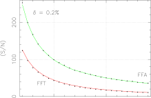
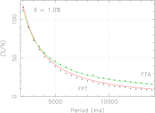
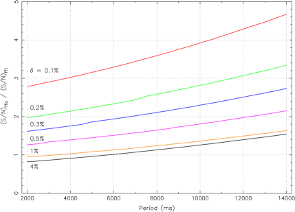
Figure 8.— Left. The signal-to-noise ratio (S/N) versus the pulsar period for two different duty cycles of $\delta=0.2\%$ (top) and $\delta=1\%$ (bottom) for both FFT and FFA searches. Results from our simulation are plotted by dots, and the dependences of S/Ns from the analytical consideration are shown by lines. Right. The “efficiency” of the FFA search versus the pulsar period and as a function of duty cycle. The “efficiency” is defined as the ratio of the S/N of the fake pulsar detected with the FFA search to the S/N of the fake pulsar detected with the FFT search. Six different curves represent the analytical dependence for different pulse duty cycles.

A.4. Testing

We have tested our program on a number of normal pulsars and on the two RRATs (J0848–43 and J1754–30) which have recently been shown to be detectable through their time-averaged emission in observations with the GBT at 350 MHz (McLaughlin, 2009a). These RRATs provide excellent tests of the FFA because they generally have rather long periods and small duty cycles that are similar to those of the XDINS. Both J0848–43 and J1754–30 were detected using both the FFA and FFT searches with S/Ns that agree well with the FFA efficiency plot shown in Fig. 8, right. Pulsar J0848$-$43 has a period of about 5.9 s and a pulse duty cycle of about 2%, which should result in roughly similar S/N detections in the FFA and FFT based on Fig. 8, right. Indeed, it was detected with S/N $\approx 16$ in the FFA search and with S/N $\approx 19$ in the FFT search. Pulsar J1754$-$30 has a period of 1.32 s and duty cycle of about 8%. As expected, it was detected with larger S/N ($\approx 44$) in the FFT search than in the FFA search ($\approx 25$). This agrees very well with our simulations that shows that the FFT search performs better for shorter periods and broader pulses.

Tests on a few other pulsars confirmed this result. As an example, PSR J0628+09, with period of 1.24 s and small duty cycle of only 0.8%, was not detected in the FFT search at all using the default incoherent sum of 32 harmonics. However, it was detected with 64 and 128 harmonics with S/N of 17.2 and 19.5, respectively, owing to increased sensitivity to narrower pulses. With the FFA it was even detected without the matched filtering technique, i.e. without optimal rebinning with smoothing window equal to the width of the pulse. Both in the FFT and FFA, the S/Ns are about the same for similar equivalent pulse widths, agreeing well with our simulation and analytical expression (see Fig. 8). The non-detection of the pulsar with the FFT using the default incoherent sum of 32 harmonics is likely due to its weakness because of the sporadic nature. This pulsar was discovered originally only in the single-pulse search (Cordes et al., 2006). Thus, in case of weak pulsars or bright but intermittent pulsars the FFA has a significant advantage against the FFT.

References

- Aguilera et al. (2008) Aguilera, D. N., Pons, J. A., & Miralles, J. A. 2008, ApJ, 673, L167
- Blaschke et al. (2004) Blaschke, D., Grigorian, H., & Voskresensky, D. N. 2004, A&A, 424, 979
- Bracewell (2000) Bracewell, R. N. 2000, The Fourier transform and its applications (Boston : McGraw Hill, McGraw-Hill series in electrical and computer engineering. Circuits and systems)
- Brazier & Johnston (1999) Brazier, K. T. S., & Johnston, S. 1999, MNRAS, 305, 671
- Burns & Clark (1969) Burns, W. R., & Clark, B. G. 1969, A&A, 2, 280
- Camilo et al. (2007) Camilo, F., Ransom, S. M., Halpern, J. P., & Reynolds, J. 2007, ApJ, 666, L93
- Camilo et al. (2006) Camilo, F., Ransom, S. M., Halpern, J. P., Reynolds, J., Helfand, D. J., Zimmerman, N., & Sarkissian, J. 2006, Nature, 442, 892
- Cordes et al. (2006) Cordes, J. M., Freire, P. C. C., Lorimer, D. R., Camilo, F., Champion, D. J., Nice, D. J., Ramachandran, R., Hessels, J. W. T., Vlemmings, W., van Leeuwen, J., Ransom, S. M., Bhat, N. D. R., Arzoumanian, Z., McLaughlin, M. A., Kaspi, V. M., Kasian, L., Deneva, J. S., Reid, B., Chatterjee, S., Han, J. L., Backer, D. C., Stairs, I. H., Deshpande, A. A., & Faucher-Giguère, C.-A. 2006, ApJ, 637, 446
- Cordes & Lazio (2002) Cordes, J. M., & Lazio, T. J. W. 2002, ArXiv Astrophysics e-prints
- Cordes & McLaughlin (2003) Cordes, J. M., & McLaughlin, M. A. 2003, ApJ, 596, 1142
- Cropper et al. (2004) Cropper, M., Haberl, F., Zane, S., & Zavlin, V. E. 2004, MNRAS, 351, 1099
- Evans et al. (2000) Evans, M., Hastings, N., & Peacock, B. 2000, Statistical Distributions (3rd ed., New York: Wiley)
- Faucher-Giguere & Kaspi (2007) Faucher-Giguere, C. ., & Kaspi, V. M. 2007, ArXiv e-prints, 710
- Gonzalez et al. (2004) Gonzalez, M. E., Kaspi, V. M., Lyne, A. G., & Pivovaroff, M. J. 2004, ApJ, 610, L37
- Gotthelf et al. (2004) Gotthelf, E. V., Halpern, J. P., Buxton, M., & Bailyn, C. 2004, ApJ, 605, 368
- Haberl (2004) Haberl, F. 2004, Advances in Space Research, 33, 638
- Haberl (2007) —. 2007, Ap&SS, 308, 181
- Haberl et al. (1997) Haberl, F., Motch, C., Buckley, D. A. H., Zickgraf, F.-J., & Pietsch, W. 1997, A&A, 326, 662
- Haberl et al. (2004a) Haberl, F., Motch, C., Zavlin, V. E., Reinsch, K., Gänsicke, B. T., Cropper, M., Schwope, A. D., Turolla, R., & Zane, S. 2004a, A&A, 424, 635
- Haberl et al. (1996) Haberl, F., Pietsch, W., Motch, C., & Buckley, D. A. H. 1996, IAU Circ., 6445, 2
- Haberl et al. (2003) Haberl, F., Schwope, A. D., Hambaryan, V., Hasinger, G., & Motch, C. 2003, A&A, 403, L19
- Haberl et al. (2006) Haberl, F., Turolla, R., de Vries, C. P., Zane, S., Vink, J., Méndez, M., & Verbunt, F. 2006, A&A, 451, L17
- Haberl & Zavlin (2002) Haberl, F., & Zavlin, V. E. 2002, A&A, 391, 571
- Haberl et al. (2004b) Haberl, F., Zavlin, V. E., Trümper, J., & Burwitz, V. 2004b, A&A, 419, 1077
- Hankins & Rickett (1975) Hankins, T. H., & Rickett, B. J. 1975, Methods in Computational Physics, 14, 55
- Haslam et al. (1982) Haslam, C. G. T., Salter, C. J., Stoffel, H., & Wilson, W. E. 1982, A&AS, 47, 1
- Ibrahim et al. (2004) Ibrahim, A. I., Markwardt, C. B., Swank, J. H., Ransom, S., Roberts, M., Kaspi, V., Woods, P. M., Safi-Harb, S., Balman, S., Parke, W. C., Kouveliotou, C., Hurley, K., & Cline, T. 2004, ApJ, 609, L21
- Johnson et al. (1994) Johnson, N., Kotz, S., & Balakrishnan, N. 1994, Continuous Univariate Distributions (Vol. 1, 2nd ed., Boston, MA: Houghton Mifflin)
- Johnston (2003) Johnston, S. 2003, MNRAS, 340, L43
- Kaplan (2008) Kaplan, D. L. 2008, in American Institute of Physics Conference Series, Vol. 968, Astrophysics of Compact Objects, ed. Y.-F. Yuan, X.-D. Li, & D. Lai, 129–136
- Kaplan et al. (2005) Kaplan, D. L., Escoffier, R. P., Lacasse, R. J., O’Neil, K., Ford, J. M., Ransom, S. M., Anderson, S. B., Cordes, J. M., Lazio, T. J. W., & Kulkarni, S. R. 2005, PASP, 117, 643
- Kaplan et al. (2002) Kaplan, D. L., Kulkarni, S. R., & van Kerkwijk, M. H. 2002, ApJ, 579, L29
- Kaplan et al. (2003a) —. 2003a, ApJ, 588, L33
- Kaplan & van Kerkwijk (2005a) Kaplan, D. L., & van Kerkwijk, M. H. 2005a, ApJ, 628, L45
- Kaplan & van Kerkwijk (2005b) —. 2005b, ApJ, 635, L65
- Kaplan & van Kerkwijk (2009) —. 2009, ApJ, 692, L62
- Kaplan et al. (2007) Kaplan, D. L., van Kerkwijk, M. H., & Anderson, J. 2007, ApJ, 660, 1428
- Kaplan et al. (2003b) Kaplan, D. L., van Kerkwijk, M. H., Marshall, H. L., Jacoby, B. A., Kulkarni, S. R., & Frail, D. A. 2003b, ApJ, 590, 1008
- Kaspi & McLaughlin (2005) Kaspi, V. M., & McLaughlin, M. A. 2005, ApJ, 618, L41
- Kramer et al. (1998) Kramer, M., Xilouris, K. M., Lorimer, D. R., Doroshenko, O., Jessner, A., Wielebinski, R., Wolszczan, A., & Camilo, F. 1998, ApJ, 501, 270
- Kulkarni & van Kerkwijk (1998) Kulkarni, S. R., & van Kerkwijk, M. H. 1998, ApJ, 507, L49
- Lorimer & Kramer (2004) Lorimer, D. R., & Kramer, M. 2004, Handbook of Pulsar Astronomy (Cambridge observing handbooks for research astronomers, Vol. 4. Cambridge, UK: Cambridge University Press)
- Lovelace et al. (1969) Lovelace, R. V. E., Sutton, J. M., & Salpeter, E. E. 1969, Nature, 222, 231
- Lyne & Manchester (1988) Lyne, A. G., & Manchester, R. N. 1988, MNRAS, 234, 477
- Maccacaro et al. (1988) Maccacaro, T., Gioia, I. M., Wolter, A., Zamorani, G., & Stocke, J. T. 1988, ApJ, 326, 680
- Malofeev et al. (2007) Malofeev, V. M., Malov, O. I., & Teplykh, D. A. 2007, Ap&SS, 308, 211
- Malofeev et al. (2005) Malofeev, V. M., Malov, O. I., Teplykh, D. A., Tyul’Bashev, S. A., & Tyul’Basheva, G. E. 2005, Astr. Rep., 49, 242
- Maron et al. (2000) Maron, O., Kijak, J., Kramer, M., & Wielebinski, R. 2000, A&AS, 147, 195
- McLaughlin (2009a) McLaughlin, M. 2009a, in Astrophysics and Space Science Library, Vol. 357, Astrophysics and Space Science Library, ed. W. Becker, 41–66
- McLaughlin et al. (2006) McLaughlin, M. A., Lyne, A. G., Lorimer, D. R., Kramer, M., Faulkner, A. J., Manchester, R. N., Cordes, J. M., Camilo, F., Possenti, A., Stairs, I. H., Hobbs, G., D’Amico, N., Burgay, M., & O’Brien, J. T. 2006, Nature, 439, 817
- McLaughlin et al. (2007) McLaughlin, M. A., Rea, N., Gaensler, B. M., Chatterjee, S., Camilo, F., Kramer, M., Lorimer, D. R., Lyne, A. G., Israel, G. L., & Possenti, A. 2007, ApJ, 670, 1307
- McLaughlin et al. (2003) McLaughlin, M. A., Stairs, I. H., Kaspi, V. M., Lorimer, D. R., Kramer, M., Lyne, A. G., Manchester, R. N., Camilo, F., Hobbs, G., Possenti, A., D’Amico, N., & Faulkner, A. J. 2003, ApJ, 591, L135
- McLaughlin et al. (2009) McLaughlin, M. A., et al. 2009, MNRAS, submitted
- Motch & Haberl (1998) Motch, C., & Haberl, F. 1998, A&A, 333, L59
- Motch et al. (1999) Motch, C., Haberl, F., Zickgraf, F.-J., Hasinger, G., & Schwope, A. D. 1999, A&A, 351, 177
- Page et al. (2006) Page, D., Geppert, U., & Weber, F. 2006, Nuclear Physics A, 777, 497
- Page et al. (2004) Page, D., Lattimer, J. M., Prakash, M., & Steiner, A. W. 2004, ApJS, 155, 623
- Perlman et al. (1996) Perlman, E. S., Stocke, J. T., Schachter, J. F., Elvis, M., Ellingson, E., Urry, C. M., Potter, M., Impey, C. D., & Kolchinsky, P. 1996, ApJS, 104, 251
- Pivovaroff et al. (2000) Pivovaroff, M. J., Kaspi, V. M., & Camilo, F. 2000, ApJ, 535, 379
- Pons & Geppert (2007) Pons, J. A., & Geppert, U. 2007, A&A, 470, 303
- Popov et al. (2006a) Popov, S., Grigorian, H., Turolla, R., & Blaschke, D. 2006a, A&A, 448, 327
- Popov et al. (2003) Popov, S. B., Colpi, M., Prokhorov, M. E., Treves, A., & Turolla, R. 2003, A&A, 406, 111
- Popov et al. (2006b) Popov, S. B., Turolla, R., & Possenti, A. 2006b, MNRAS, 369, L23
- Posselt et al. (2007) Posselt, B., Popov, S. B., Haberl, F., Trümper, J., Turolla, R., & Neuhäuser, R. 2007, Ap&SS, 308, 171
- Radhakrishnan & Cooke (1969) Radhakrishnan, V., & Cooke, D. J. 1969, Astrophys. Lett., 3, 225
- Ransom et al. (2002) Ransom, S. M., Eikenberry, S. S., & Middleditch, J. 2002, AJ, 124, 1788
- Rea et al. (2007) Rea, N., Torres, M. A. P., Jonker, P. G., Mignani, R. P., Zane, S., Burgay, M., Kaplan, D. L., Turolla, R., Israel, G. L., & Steeghs, D. 2007, MNRAS, 379, 1484
- Rutledge et al. (2008) Rutledge, R. E., Fox, D. B., & Shevchuk, A. H. 2008, ApJ, 672, 1137
- Schwope et al. (2009) Schwope, A. D., Erben, T., Kohnert, J., Lamer, G., Steinmetz, M., Strassmeier, K., Zinnecker, H., Bechtold, J., Diolaiti, E., Fontana, A., Gallozzi, S., Giallongo, E., Ragazzoni, R., de Santis, C., & Testa, V. 2009, A&A, 499, 267
- Schwope et al. (1999) Schwope, A. D., Hasinger, G., Schwarz, R., Haberl, F., & Schmidt, M. 1999, A&A, 341, L51
- Staelin (1969) Staelin, D. H. 1969, IEEE Proceedings, 57, 724
- Tauris & Manchester (1998) Tauris, T. M., & Manchester, R. N. 1998, MNRAS, 298, 625
- Tiengo & Mereghetti (2007) Tiengo, A., & Mereghetti, S. 2007, ApJ, 657, L101
- Treves et al. (2000) Treves, A., Turolla, R., Zane, S., & Colpi, M. 2000, PASP, 112, 297
- van Kerkwijk & Kaplan (2007) van Kerkwijk, M. H., & Kaplan, D. L. 2007, Ap&SS, 308, 191
- van Kerkwijk & Kaplan (2008) —. 2008, ApJ, 673, L163
- van Kerkwijk et al. (2004) van Kerkwijk, M. H., Kaplan, D. L., Durant, M., Kulkarni, S. R., & Paerels, F. 2004, ApJ, 608, 432
- Voges et al. (1999) Voges, W., Aschenbach, B., Boller, T., Bräuninger, H., Briel, U., Burkert, W., Dennerl, K., Englhauser, J., Gruber, R., Haberl, F., Hartner, G., Hasinger, G., Kürster, M., Pfeffermann, E., Pietsch, W., Predehl, P., Rosso, C., Schmitt, J. H. M. M., Trümper, J., & Zimmermann, H. U. 1999, A&A, 349, 389
- Vranesevic et al. (2004) Vranesevic, N., Manchester, R. N., Lorimer, D. R., Hobbs, G. B., Lyne, A. G., Kramer, M., Camilo, F., Stairs, I. H., Kaspi, V. M., D’Amico, N., Possenti, A., Crawford, F., Faulkner, A. J., & McLaughlin, M. A. 2004, ApJ, 617, L139
- Walter & Lattimer (2002) Walter, F. M., & Lattimer, J. M. 2002, ApJ, 576, L145
- Walter & Matthews (1997) Walter, F. M., & Matthews, L. D. 1997, Nature, 389, 358
- Walter et al. (1996) Walter, F. M., Wolk, S. J., & Neuhäuser, R. 1996, Nature, 379, 233
- Weltevrede et al. (2007) Weltevrede, P., Stappers, B. W., Rankin, J. M., & Wright, G. A. E. 2007, ArXiv Astrophysics e-prints
- Weltevrede et al. (2006) Weltevrede, P., Wright, G. A. E., Stappers, B. W., & Rankin, J. M. 2006, A&A, 458, 269
- Wolszczan (1991) Wolszczan, A. 1991, Nature, 350, 688
- Yakovlev & Pethick (2004) Yakovlev, D. G., & Pethick, C. J. 2004, ARA&A, 42, 169
- Zampieri et al. (2001) Zampieri, L., Campana, S., Turolla, R., Chieregato, M., Falomo, R., Fugazza, D., Moretti, A., & Treves, A. 2001, A&A, 378, L5
- Zane et al. (2005) Zane, S., Cropper, M., Turolla, R., Zampieri, L., Chieregato, M., Drake, J. J., & Treves, A. 2005, ApJ, 627, 397
- Zane et al. (2006) Zane, S., de Luca, A., Mignani, R. P., & Turolla, R. 2006, A&A, 457, 619
- Zane et al. (2008) Zane, S., Mignani, R. P., Turolla, R., Treves, A., Haberl, F., Motch, C., Zampieri, L., & Cropper, M. 2008, ApJ, 682, 487