abbr
Global entrainment of transcriptional systems to periodic inputs
ABSTRACT
This paper addresses the problem of giving conditions for transcriptional systems to be globally entrained to external periodic inputs. By using contraction theory, a powerful tool from dynamical systems theory, it is shown that certain systems driven by external periodic signals have the property that all solutions converge to a fixed limit cycle. General results are proved, and the properties are verified in the specific case of some models of transcriptional systems.
1 Introduction
Periodic, clock-like rhythms pervade nature and regulate the function of all living organisms. For instance, circadian rhythms are regulated by an endogenous biological clock entrained by the light signals from the environment that then acts as a pacemaker, [Gon_Ber_Wal_Kra_Her_05]. Moreover, such an entrainment can be obtained even if daily variations are present, like e.g. temperature and light variations. Another important example of entrainment in biological systems is at the molecular level, where the synchronization of several cellular processes is regulated by the cell cycle [Tys_Csi_Now_02].
An important question in mathematical and computational biology is that of finding conditions ensuring that entrainment occurs. The objective is to identify classes of biological systems that can be entrained by an exogenous signal. To solve this problem, modelers often resort to simulations in order to show the existence of periodic solutions in the system of interest. Simulations, however, can never prove that solutions will exist for all parameter values, and they are subject to numerical errors. Moreover, robustness of entrained solutions needs to be checked in the presence of noise and uncertainties, which cannot be avoided experimentally.
From a mathematical viewpoint, the problem of formally showing that entrainment takes place is known to be very difficult. Indeed, if a stable linear time-invariant model is used to represent the system of interest, then entrainment is usually expected, when the system is driven by an external periodic input, with the system response being a filtered, shifted version of the external driving signal. However, in general, as is often the case in biology, models are nonlinear. The response of nonlinear systems to periodic inputs is the subject of much current systems biology experimentation; for example, in [MeMu:08], the case of a cell signaling system driven by a periodic square-wave input is considered. From measurements of a periodic output, the authors fit a transfer function to the system, implicitly modeling the system as linear even though (as stated in the Suppemental Materials to [MeMu:08]) there are saturation effects so the true system is nonlinear. For nonlinear systems, driving the system by an external periodic signal does not guarantee the system response to also be a periodic solution, as nonlinear systems can exhibit harmonic generation or suppression and complex behaviour such as chaos or quasiperiodic solutions [Ku:98]. This may happen even if the system is well-behaved with respect to constant inputs; for example, there are systems which converge to a fixed steady state no matter what is the input excitation, so long as this input signal is constant, yet respond chaotically to the simplest oscillatory input; we outline such an example in an Appendix to this paper, see also [eds:arxiv09]. Thus, a most interesting open problem is that of finding conditions for the entrainment to external inputs of biological systems modelled by sets of nonlinear differential equations.
One approach to analyzing the convergence behavior of nonlinear dynamical systems is to use Lyapunov functions. However, in biological applications, the appropriate Lyapunov functions are not always easy to find and, moreover, convergence is not guaranteed in general in the presence of noise and/or uncertainties. Moreover, such an approach can be hard to apply to the case of non-autonomous systems (that is, dynamical systems directly dependent on time), as is the case when dealing with periodically forced systems.
The above limitations can be overcome if the convergence problem is interpreted as a property of all trajectories, asking that all solutions converge towards one another (contraction). This is the viewpoint of contraction theory, [Loh_Slo_98], [Loh_Slo_00], and more generally incremental stability methods [Ang_02]. Global results are possible, and these are robust to noise, in the sense that, if a system satisfies a contraction property then trajectories remain bounded in the phase space [Pha_Tab_Slo_09]. Contraction theory has a long history. Contractions in metric functional spaces can be traced back to the work of Banach and Caccioppoli [Gra_03] and, in the field of dynamical systems, to [Hartmann] and even to [Lewis] (see also [Pav_Pog_Wou_Nij], [Ang_02], and e.g. [pde] for a more exhaustive list of related references). Contraction theory has been successfully applied to both nonlinear control and observer problems, [Loh_Slo_00], [Jou_04_a] and, more recently, to synchronization and consensus problems in complex networks [Slo_Wan_Rif_98], [Wan_Slo_05]. In [Rus_diB_09b] it was proposed that contraction can be particularly useful when dealing with the analysis and characterization of biological networks. In particular, it was found that using non Euclidean norms can be particularly effective in this context [Rus_diB_09b], [Rus_diB_09].
One of the objectives of this paper is to give a self-contained exposition, with all proofs included, of results in contraction theory as applied to entrainment of periodic signals, and, moreover, to show their applicability to a problem of biological interest, having to do with a driven transcriptional system. A surprising fact is that, for these applications, and contrary to many engineering aplications, norms other than Euclidean, and associated matrix measures, must be considered.
1.1 Mathematical tools
We consider in this paper systems of ordinary differential equations, generally time-dependent:
| (1) |
defined for and , where is a subset of . It will be assumed that is differentiable on , and that , as well as the Jacobian of with respect to , denoted as , are both continuous in . In applications of the theory, it is often the case that will be a closed set, for example given by non-negativity constraints on variables as well as linear equalities representing mass-conservation laws. For a non-open set , differentiability in means that the vector field can be extended as a differentiable function to some open set which includes , and the continuity hypotheses with respect to hold on this open set.
We denote by the value of the solution at time of the differential equation (1) with initial value . It is implicit in the notation that (“forward invariance” of the state set ). This solution is in principle defined only on some interval , but we will assume that is defined for all . Conditions which guarantee such a “forward-completeness” property are often satisfied in biological applications, for example whenever the set is closed and bounded, or whenever the vector field is bounded. (See Appendix C in [mct] for more discussion, as well as [angeli-sontag-fc] for a characterization of the forward completeness property.) Under the stated assumptions, the function is jointly differentiable in all its arguments (this is a standard fact on well-posedness of differential equations, see for example Apendix C in [mct]).
We recall (see for instance [michelbook]) that, given a vector norm on Euclidean space (), with its induced matrix norm , the associated matrix measure is defined as the directional derivative of the matrix norm, that is,
For example, if is the standard Euclidean 2-norm, then is the maximum eigenvalue of the symmetric part of . As we shall see, however, different norms will be useful for our applications. Matrix measures are also known as “logarithmic norms”, a concept independently introduced by Germund Dahlquist and Sergei Lozinskii in 1959, [dahlquist, lozinskii]. The limit is known to exist, and the convergence is monotonic, see [strom, dahlquist].
We will say that system (1) is infinitesimally contracting on a convex set if there exists some norm in , with associated matrix measure such that, for some constant ,
| (2) |
Let us discuss very informally (rigorous proofs are given later) the motivation for this concept. Since by assumption is continuously differentiable, the following exact differential relation can be obtained from (1):
| (3) |
where, as before, denotes the Jacobian of the vector field , as a function of and . (The object can be thought of as a “virtual displacement” in the language of mechanics, as in [Arn_78], which views such displacements as linear tangent differential forms differentiable with respect to time.) Consider now two neighboring trajectories of (1), evolving in , and the virtual displacements between them. Note that (3) can be seen as a linear time-varying dynamical system of the form:
Hence, an upper bound for the magnitude of its solutions can be obtained by means of the Coppel inequality [Vid_93], yielding:
| (4) |
where is the matrix measure of the system Jacobian induced by the norm being considered on the states and . Using (4) and (2), we have that
Thus, trajectories starting from infinitesimally close initial conditions converge exponentially towards each other. In what follows we will refer to as contraction (or convergence) rate.
The key theoretical result about contracting systems links infinitesimal and global contractivity, and is stated below. This result can be traced, under different technical assumptions, to e.g. [Loh_Slo_98], [Pav_Pog_Wou_Nij], [Lewis], [Hartmann].
Theorem 1.
Suppose that is a convex subset of and that is infinitesimally contracting with contraction rate . Then, for every two solutions and of (1), it holds that:
| (5) |
In other words, infinitesimal contractivity implies global contractivity. In the Appendix, we provide a self-contained proof of Theorem 1. In fact, the result is shown there in a generalized form, in which convexity is replaced by a weaker constraint on the geometry of the space.
In actual applications, often one is given a system which depends implicitly on the time, , by means of a continuous function , i.e. systems dynamics are represented by . In this case, (where is some subset of ), represents an external input. It is important to observe that the contractivity property does not require any prior information about this external input. In fact, since does not depend on the system state variables, when checking the property, it may be viewed as a constant parameter, . Thus, if contractivity of holds uniformly , then it will also hold for .
Given a number , we will say that system (1) is -periodic if it holds that
Notice that the system is -periodic, if the external input, , is itself a periodic function of period .
The following is the basic theoretical result about periodic orbits that will be used in the paper. It may be found, under various different technical variants, in the references given above.
Theorem 2.
Suppose that:
-
•
is a closed convex subset of ;
-
•
is infinitesimally contracting with contraction rate ;
-
•
is -periodic.
Then, there is a unique periodic solution of (1) of period and, for every solution , it holds that as .
In the Appendix of this paper, we provide a self-contained proof of Theorem 2, in a generalized form which does not require convexity.
1.2 A simple example
As a first example to illustrate the application of the concepts introduced so far, we choose a simple bimolecular reaction, in which a molecule of and one of can reversibly combine to produce a molecule of .
This system can be modeled by the following set of differential equations:
| (6) |
where we are using to denote the concentration of and so forth. The system evolves in the positive orthant of . Solutions satisfy (stoichiometry) constraints:
| (7) |
for some constants and .
We will assume that one or both of the “kinetic constants” are time-varying, with period . Such a situation arises when the ’s depend on concentrations of additional enzymes, which are available in large amounts compared to the concentrations of , but whose concentrations are periodically varying. The only assumption will be that and for all .
Because of the conservation laws (7), we may restrict our study to the equation for . Once that all solutions of this equation are shown to globally converge to a periodic orbit, the same will follow for and . We have that:
| (8) |
Because and , this system is studied on the subset of defined by . The equation can be rewritten as:
| (9) |
Differentiation with respect to of the right-hand side in the above system yields this () Jacobian:
| (10) |
Since we know that and , it follows that
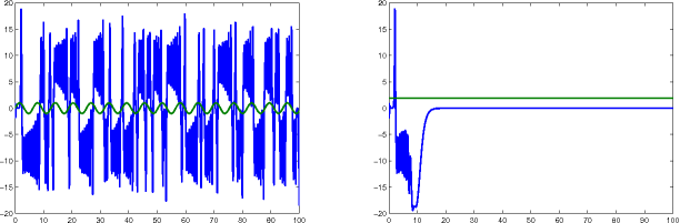
for . Using any norm (this example is in dimension one) we have that . So (6) is contracting and, by means of Theorem 2, solutions will globally converge to a unique solution of period (notice that such a solution depends on system parameters).
Figure 1 shows the behavior of the dynamical system (9), using two different values of . Notice that the asymptotic behavior of the system depends on the particular choice of the biochemical parameters being used. Furthermore, it is worth noticing here that the higher the value of , the faster will be the convergence to the attractor.
2 Results
2.1 Mathematical model and problem statement
We study a general externally-driven transcriptional module. We assume that the rate of production of a transcription factor is proportional to the value of a time dependent input function , and is subject to degradation and/or dilution at a linear rate. (Later, we generalize the model to also allow nonlinear degradation as well.) The signal might be an external input, or it might represent the concentration of an enzyme or of a second messenger that activates . In turn, drives a downstream transcriptional module by binding to a promoter (or substrate), denoted by , whose free concentration is denoted as . The binding reaction of with is reversible and given by:
where is the complex protein-promoter, and the binding and dissociation rates are and respectively. As the promoter is not subject to decay, its total concentration, , is conserved, so that the following conservation relation holds:
| (11) |
We wish to study the behavior of solutions of the system that couples and , and specifically to show that, when the input is periodic with period , this coupled system has the property that all solutions converge to some globally attracting limit cycle whose period is also .
Such transcriptional modules are ubiquitous in biology, natural as well as synthetic, and their behavior was recently studied in [DelV_Nin_Son_08] in the context of “retroactivity” (impedance or load) effects. If we think of as the concentration of a protein that is a transcription factor for , and we ignore fast mRNA dynamics, such a system can be schematically represented as in Figure 2,
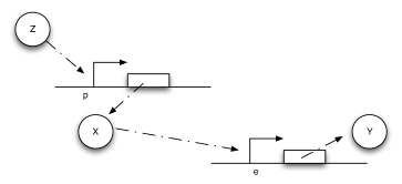
which is adapted from [DelV_Nin_Son_08]. Notice that here does not need to be the concentration of a transcriptional activator of for our results to hold. The results will be valid for any mathematical model for the concentrations, , of and , of (the concentration of is conserved) of the form:
| (12) |
Our main objective in this paper is, thus, to show that, when is a periodic input, all solutions of system (12) converge to a (unique) limit cycle (Figure 3). The key tool in this analysis is to show that, when no input is present, the system is infinitesimally, and hence globally, contracting.
Thus, the main step will be to establish the following technical result, see Section 2.2:
Theorem 3.
The system
where
| (13) |
for all , and , , , and are arbitrary positive constants, is contracting.
By means of Theorem 2, we then have the following immediate Corollary:
Theorem 4.
For any given nonnegative periodic input of period , all solutions of system (12) converge exponentially to a periodic solution of period .
In the following sections, we introduce a matrix measure that will help establish contractivity, and we prove Theorem 3. We will also discuss several extensions of this result, allowing the consideration of multiple driven subsystems as well as more general nonlinear systems with a similar structure.
2.2 Proof of Theorem 3
We will use Theorem 2. The Jacobian matrix to be studied is:
| (14) |
As matrix measure, we will use the measure induced by the vector norm , where is a suitable nonsingular matrix. More specifically, we will pick diagonal:
| (15) |
where and are two positive numbers to be appropriately chosen depending on the parameters defining the system.
It follows from general facts about matrix norms that
| (16) |
where is the measure associated to the norm and is explicitly given by the following formula:
| (17) |
Observe that, if the entries of are negative, then asking that amounts to a column diagonal dominance condition. (The above formula is for real matrices. If complex matrices would be considered, then the term should be replaced by its real part .)
Thus, the first step in computing is to calculate :
| (18) |
Using (17), we obtain:
| (19) |
Note that we are not interested in calculating the exact value for the above measure, but just in ensuring that it is negative. To guarantee that , the following two conditions must hold:
| (20) |
| (21) |
Thus, the problem becomes that of checking if there exists an appropriate range of values for , that satisfy (20) and (21) simultaneously.
The left hand side of (21) can be written as:
| (22) |
which is negative if and only if . In particular, in this case we have:
The idea is now to ensure negativity of (20) by using appropriate values for and which fulfill the above constraint. Recall that the term because of the choice of the state space (this quantity represents a concentration). Thus, the left hand side of (20) becomes
| (23) |
The next step is to choose appropriately and (without violating the constraint ). Imposing , , (23) becomes
| (24) |
Then, we have to choose an appropriate value for in order to make the above quantity uniformly negative. In particular, (24) is uniformly negative if and only if
| (25) |
We can now choose
with . In this case, (24) becomes
Thus, choosing and , with , we have . Furthermore, the contraction rate , is given by:
Notice that depends on both system parameters and on the elements , , i.e. it depends on the particular metric chosen to prove contraction. This completes the proof of the Theorem. ∎
2.3 Generalizations
In this Section, we discuss various generalizations that use the same proof technique.
2.3.1 Assuming activation by enzyme kinetics
The previous model assumed that was created in proportion to the amount of external signal . While this may be a natural assumption if is a transcription factor that controls the expression of , a different model applies if, instead, the “active” form is obtained from an “inactive” form , for example through a phosphorylation reaction which is catalyzed by a kinase whose abundance is represented by . Suppose that can also be constitutively deactivated. Thus, the complete system of reactions consists of
together with
where the forward reaction depends on . Since the concentrations of must remain constant, let us say at a value , we eliminate and have:
| (26) |
We will prove that if is periodic and positive, i.e. , then a globally attracting limit cycle exists. Namely, it will be shown, after having performed a linear coordinate transformation, that there exists a negative matrix measure for the system of interest.
Consider, indeed, the following change of the state variables:
| (27) |
The systems dynamics, then become:
| (28) |
As matrix measure, we will now use the measure induced by the vector norm . (Notice that this time, the matrix is the identity matrix).
Given a real matrix , the matrix measure is explicitly given by the following formula (see e.g. [michelbook]):
| (29) |
(Observe that this is a row-dominance condition, in contrast to the dual column-dominance condition used for .)
Differentiation of (28) yields the Jacobian matrix:
Thus, it immediately follow from (29) that is negative if and only if:
| (30) |
| (31) |
The first inequality is clearly satisfied since by hypotheses both system parameters and the periodic input are positive. In particular, we have:
By using (27) (recall that ), the right hand side of the second inequality can be written as:
Since all system parameters are positive and , the above quantity is negative and upper bounded by .
Thus, we have that , where:
The contraction property for the system is then proved. By means of Theorem 2, we can then conclude that the system can be entrained by any periodic input.
Simulation results are presented in Figure 4, where the presence of a stable limit cycle having the same period as is shown.
2.3.2 Multiple driven systems
We may also treat the case in which the species regulates multiple downstream transcriptional modules which act independently from each other, as shown in Figure 5.
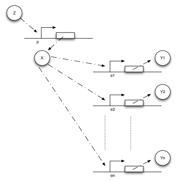
The biochemical parameters defining the different downstream modules may be different from each other, representing a situation in which the transcription factor regulates different species. After proving a general result on oscillations, and assuming that parameters satisfy the retroactivity estimates discussed in [DelV_Nin_Son_08], one may in this fashion design a single input-multi output module in which e.g. the outputs are periodic functions with different mean values, settling times, and so forth.
We denote by the various promoters, and use to denote the concentrations of the respective promoters complexed with . The resulting mathematical model becomes:
| (32) |
We consider the corresponding system with no input first, assuming that the states satisfy and for all .
Our generalization can be stated as follows:
Theorem 5.
System (32) with no input (i.e. ) is contracting. Hence, if is a non-zero periodic input, its solutions exponentially converge towards a periodic orbit of the same period as .
Proof.
We only outline the proof, since it is similar to the proof of Theorem 4. We employ the following matrix measure:
| (33) |
where
| (34) |
and the scalars have to be chosen appropriately ().
In this case,
| (35) |
and
| (36) |
Hence, the inequalities to be satisfied are:
| (37) |
and
| (38) |
Clearly, the set of inequalities above admits a solution. Indeed, the left hand side of (38) can be recast as
which is negative definite if and only if for all . Specifically, in this case we have
Also, from (37), as for all , we have that (37) can be rewritten as:
Since , we can impose (with ) and the above inequality becomes
Clearly, such inequality is satisfied if we choose sufficiently small; namely:
In Figure 6 the behavior of two-driven downstream transcriptional modules is shown. Notice that both the downstream modules are entrained by the periodic input , but their steady state behavior is different.
Notice that, by the same arguments used above, it can be proven that
| (39) |
is contracting.
2.3.3 Transcriptional cascades
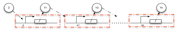
A cascade of (infinitesimally) contracting systems is also (infinitesimally) contracting (see Appendix D for the proof). This implies that any transcriptional cascade, will also give rise to a contracting system, and, in particular, will entrain to periodic inputs. By a transcriptional cascade we mean a system as shown in Figure 7. In this figure, we interpret the intermediate variables as transcription factors, making the simplifying assumption that TF concentration is proportional to active promoter for the corresponding gene. (More complex models, incorporating transcription, translation, and post-translational modifications could themselves, in turn, be modeled as cascades of contracting systems.)
2.3.4 More abstract systems
We can extend our results even further, to a larger class of nonlinear systems, as long as the same general structure is present. This can be useful for example to design new synthetic transcription modules or to analyze the entrainment properties of general biological systems. We start with a discussion of a two dimensional system of the form:
| (40) |
In molecular biology, would typically represent a nonlinear degradation, for instance in Michaelis-Menten form, while the function represents the interaction between and . The aim of this Section is to find conditions on the degradation and interaction terms that allow one to show contractivity of the unforced (no input ) system, and hence existence of globally attracting limit cycles.
We assume that the state space is compact (closed and bounded) as well as convex.
Theorem 6.
System (40), without inputs , evolving on a convex compact subset of phase space is contracting, provided that the following conditions are all satisfied, for each :
-
•
;
-
•
;
-
•
does not change sign;
-
•
.
Notice that the last condition is automatically satisfied if , because .
Proof.
As before, we prove contraction by constructing an appropriate negative measure for the Jacobian of the vector field. In this case, the Jacobian matrix is:
| (41) |
Once again, as matrix measure we will use:
| (42) |
with
| (43) |
and appropriately chosen.
Using (42) we have
| (44) |
Following the same steps as the proof of Theorem 3, we have to show that:
| (45) |
| (46) |
Clearly, if for every and , the first inequality is satisfied, with
To prove the theorem we need to show that there exists and satisfying (46). For such inequality, since does not change sign in by hypothesis, we have two possibilities:
-
1.
, ;
-
2.
, .
In the first case, the right hand side of (46) becomes
| (47) |
Choosing , with , we have:
Specifically, if we now pick
where and , we have that the above quantity is uniformly negative definite, i.e.
In the second case, the right hand side of (46) becomes
| (48) |
Again, by choosing , with , we have the following upper bound for the expression in (48):
| (49) |
Thus, it follows that provided that the above quantity is uniformly negative definite. Since, by hypotheses,
| (50) |
then . The proof of the Theorem is now complete. ∎
From a biological viewpoint, the hardest hypothesis to satisfy in Theorem 6 might be that on the derivatives of . However, it is possible to relax the hypothesis on if the rate of change of with respect to , i.e. , is sufficiently larger than . In particular, the following result can be proved.
Theorem 7.
System (40), without inputs , evolving on a convex compact set, is contractive provided that:
-
•
, ;
-
•
, ;
-
•
.
Proof.
The proof is similar to that of Theorem 6. In particular, we can repeat the same derivation to obtain again inequality (46). Thence, as no hypothesis is made on the sign of , choosing we have
| (51) |
Thus, it follows that, if , then such that , implying contractivity. The above condition is satisfied by hypotheses, hence the theorem is proved. ∎
Remarks
Theorems 6 and 7 show the possibility of designing with high flexibility the self-degradation and interaction functions for an input-output module.
This flexibility can be further increased, for example in the following ways:
3 Materials and Methods
All simulations are performed in MATLAB (Simulink), Version 7.4, with variable step ODE solver ODE23t. Simulink models are available upon request.
4 Conclusions
We have presented a systematic methodology to derive conditions for transcriptional modules to be globally entrained to periodic inputs. By means of contraction theory, a useful tool from dynamical systems, we showed that it is possible to use non-Euclidean norms and their associated matrix measures to characterize the behavior of several modules when subject to external periodic excitations. Specifically, starting with a simple bimolecular reaction, we considered the case of a general externally-driven transcriptional module and extended the analysis to some important generalizations including the case of multiple driven systems. In all cases conditions are derived by proving that the module of interest is contracting under some generic assumptions on its parameters. The importance of the results presented in the paper from a design viewpoint are also discussed by means of more abstract systems where generic nonlinear degradation and interaction terms are assumed.
References
- [1] \harvarditemAngeli2002Ang_02 Angeli, D. \harvardyearleft2002\harvardyearright. A Lyapunov approach to incremental stability properties, IEEE Transactions on Automatic Control 47: 410–321.
- [2] \harvarditemAngeli \harvardand Sontag1999angeli-sontag-fc Angeli, D. \harvardand Sontag, E. D. \harvardyearleft1999\harvardyearright. Forward completeness, unboundedness observability, and their Lyapunov characterizations, Systems and Control Letters 38: 209–217.
- [3] \harvarditemArnold1978Arn_78 Arnold, V. I. \harvardyearleft1978\harvardyearright. Mathematical methods of classical mechanics, Springer-Verlag (New York).
- [4] \harvarditem[Del Vecchio et al.]DelVecchio, Ninfa \harvardand Sontag2008DelV_Nin_Son_08 Del Vecchio, D., Ninfa, A. J. \harvardand Sontag, E. D. \harvardyearleft2008\harvardyearright. Modular cell biology: retroactivity and insulation, Nature Molecular Systems Biology 4: 161.
- [5] \harvarditemDahlquist1959dahlquist Dahlquist, G. \harvardyearleft1959\harvardyearright. Stability and error bounds in the numerical integration of ordinary differential equations, Trans. Roy. Inst. Techn. (Stockholm).
- [6] \harvarditem[Gonze et al.]Gonze, Bernard, Walterman, Kramer \harvardand Herzerl2005Gon_Ber_Wal_Kra_Her_05 Gonze, D., Bernard, S., Walterman, C., Kramer, A. \harvardand Herzerl, H. \harvardyearleft2005\harvardyearright. Spontaneous synchronization of coupled circadian oscillators, Biophysical Journal 89: 120–129.
- [7] \harvarditemGranas \harvardand Dugundji2003Gra_03 Granas, A. \harvardand Dugundji, J. \harvardyearleft2003\harvardyearright. Fixed Point Theory, Springer-Verlag (New York).
- [8] \harvarditemHartman1961Hartmann Hartman, P. \harvardyearleft1961\harvardyearright. On stability in the large for systems of ordinary differential equations, Canadian Journal of Mathematics 13: 480–492.
- [9] \harvarditemJouffroy \harvardand Slotine2004Jou_04_a Jouffroy, J. \harvardand Slotine, J. J. E. \harvardyearleft2004\harvardyearright. Methodological remarks on contraction theory, 42nd Conf. Decision and Control: 2537-2543, IEEE Press.
- [10] \harvarditemKuznetsov2004Ku:98 Kuznetsov, Y. A. \harvardyearleft2004\harvardyearright. Elements of applied bifurcation theory, Springer-Verlag (New York).
- [11] \harvarditemLewis1949Lewis Lewis, D. C. \harvardyearleft1949\harvardyearright. Metric properties of differential equations, American Journal of Mathematics 71: 294–312.
- [12] \harvarditemLohmiller \harvardand Slotine2005pde Lohmiller, W. \harvardand Slotine, J. J. \harvardyearleft2005\harvardyearright. Contraction analysis of non-linear distributed systems, International Journal of Control 78: 678–688.
- [13] \harvarditemLohmiller \harvardand Slotine1998Loh_Slo_98 Lohmiller, W. \harvardand Slotine, J. J. E. \harvardyearleft1998\harvardyearright. On contraction analysis for non-linear systems, Automatica 34: 683–696.
- [14] \harvarditemLohmiller \harvardand Slotine2000Loh_Slo_00 Lohmiller, W. \harvardand Slotine, J. J. E. \harvardyearleft2000\harvardyearright. Nonlinear process control using contraction theory, AIChe Journal 46: 588–596.
- [15] \harvarditemLozinskii1959lozinskii Lozinskii S. M. \harvardyearleft1959\harvardyearright. Error estimate for numerical integration of ordinary differential equations. I, Izv. Vyssh. Uchebn. Zaved. Mat. 5: 222–222.
- [16] \harvarditem[Mettetal et al.]Mettetal, Muzzey, Gomez-Uribe \harvardand van Oudenaarden2008MeMu:08 Mettetal, J. T., Muzzey, D., Gomez-Uribe, C. \harvardand van Oudenaarden, A. \harvardyearleft2008\harvardyearright. The frequency dependence of osmo-adaptation in Saccharomyces Cerevisiae, Science 319: 482–484.
- [17] \harvarditemMichel et al.2007michelbook Michel, A. N., Liu D., \harvardand Hou, L. \harvardyearleft2007\harvardyearright. Stability of Dynamical Systems: Continuous, Discontinuous, and Discrete Systems, Springer-Verlag (New York).
- [18] \harvarditem[Pavlov et al.]Pavlov, Pogromvsky, van de Wouv \harvardand Nijmeijer2004Pav_Pog_Wou_Nij Pavlov, A., Pogromvsky, A., van de Wouv, N. \harvardand Nijmeijer, H. \harvardyearleft2004\harvardyearright. Convergent dynamics, a tribute to Boris Pavlovich Demidovich, Systems and Control Letters 52: 257–261.
- [19] \harvarditem[Pham et al.]Pham, Tabareau \harvardand Slotine2009Pha_Tab_Slo_09 Pham, Q. C., Tabareau, N. \harvardand Slotine, J. J. E. \harvardyearleft2009\harvardyearright. A contraction theory approach to stochastic incremental stability, IEEE Transactions on Automatic Control 54: 816-820.
- [20] \harvarditem[Russo and di Bernardo]Russo \harvardand di Bernardo2009Rus_diB_09b Russo, G. \harvardand di Bernardo, M.. \harvardyearleft2009\harvardyearright. How to synchronize biological clocks, Journal of Computational Biology 16: 379–393.
- [21] \harvarditem[Russo and di Bernardo]Russo \harvardand di Bernardo2009bRus_diB_09 Russo, G. \harvardand di Bernardo, M.. \harvardyearleft2009\harvardyearright. An algorithm for the construction of synthetic self synchronizing biological circuits, Proceedings of the International Symposium on Circuits and Systems, to appear.
- [22] \harvarditem[Slotine et al.]Slotine, Wang \harvardand Rifai2004Slo_Wan_Rif_98 Slotine, J. J. E., Wang, W. \harvardand Rifai, K. E. \harvardyearleft2004\harvardyearright. Contraction analysis of synchronization of nonlinearly coupled oscillators, 16th International Symposium on Mathematical Theory of Networks and Systems, Katholieke Universiteit Leuven, Belgium, July 5-9.
- [23] \harvarditemSontag1998mct Sontag, E. D. \harvardyearleft1998\harvardyearright. Mathematical Control Theory. Deterministic Finite-Dimensional Systems, Springer-Verlag (New York).
- [24] \harvarditemSontag2009eds:arxiv09 Sontag, E. D. \harvardyearleft2009\harvardyearright. An observation regarding systems which converge to steady states for all constant inputs, yet become chaotic with periodic inputs, Technical Report, http://arxiv.org/abs/0906.2166
- [25] \harvarditem[Strom]Strom1975strom Strom, T. \harvardyearleft1975\harvardyearright. On logarithmic norms, SIAM J. Numer. Anal. 12: 741–753.
- [26] \harvarditem[Tyson et al.]Tyson, Csikasz-Nagy \harvardand Novak2002Tys_Csi_Now_02 Tyson, J. J., Csikasz-Nagy, A. \harvardand Novak, B. \harvardyearleft2002\harvardyearright. The dynamics of cell cycle regulation, Bioessays 24: 1095–1109.
- [27] \harvarditemVidyasagar1993Vid_93 Vidyasagar, M. \harvardyearleft1993\harvardyearright. Nonlinear systems analysis (2nd Ed.), Pretice-Hall (Englewood Cliffs, NJ).
- [28] \harvarditemWang \harvardand Slotine2005Wan_Slo_05 Wang, W. \harvardand Slotine, J. J. E. \harvardyearleft2005\harvardyearright. On partial contraction analysis for coupled nonlinear oscillators, Biological Cybernetics 92: 38–53.
- [29]
Appendix A -reachable sets
We will make use of the following definition:
Definition 1.
Let be any positive real number. A subset is -reachable if, for any two points and in there is some continuously differentiable curve such that:
-
1.
,
-
2.
and
-
3.
, .
For convex sets , we may pick , so and we can take . Thus, convex sets are -reachable, and it is easy to show that the converse holds as well.
Notice that a set is -reachable for some if and only if the length of the geodesic (smooth) path (parametrized by arc length), connecting any two points and in , is bounded by some multiple of the Euclidean norm, . Indeed, re-parametrizing to a path defined on , we have:
Since in finite dimensional spaces all the norms are equivalent, then it is possible to obtain a suitable for Definition 1.
Remark 1.
The notion of -reachable set is weaker that that of convex set. Nonetheless, in Theorem 8, we will prove that trajectories of a smooth system, evolving on a -reachable set, converge towards each other, even if is not convex. This additional generality allows one to establish contracting behavior for systems evolving on phase spaces exhibiting “obstacles”, as are frequently encountered in path-planing problems, for example. A mathematical example of a set with obstacles follows.
Example 1.
Consider the two dimensional set, , defined by the following contraints:
Clearly, is a non-convex subset of . We claim that is -reachable, for any positive real number . Indeed, given any two points and in , there are two possibilities: either the segment connecting and is in , or it intersects the unit circle. In the first case, we can simply pick the segment as a curve (). In the second case, one can consider a straight segment that is modified by taking the shortest perimiter route around the circle; the length of the perimeter path is at most times the length of the omitted segment. (In order to obtain a differentiable, instead of merely a piecewise-differentiable, path, an arbitrarily small increase in is needed.)
Appendix B Proof of Theorem 1
We now prove the main result on contracting systems, i.e. Theorem 1, under the hypotheses that the set , i.e. the set on which the system evolves, is -reachable.
Theorem 8.
Suppose that is a -reachable subset of and that is infinitesimally contracting with contraction rate . Then, for every two solutions and it holds that:
| (53) |
Proof.
Given any two points and in , pick a smooth curve , such that and . Let , that is, the solution of system (1) rooted in , . Since and are continuously differentiable, also is continuously differentiable in both arguments. We define
It follows that
Now,
so, we have:
| (54) |
where . Using Coppel’s inequality [Vid_93], yields
| (55) |
, , and . Notice the Fundamental Theorem of Calculus, we can write
Hence, we obtain
Now, using (55), the above inequality becomes:
The Theorem is then proved. ∎
Appendix C Proof of Theorem 2
In this Section we assume that the vector field is -periodic and prove Theorem 2.
Before starting with the proof of Theorem 2 we make the following:
Remark 2.
Periodicity implies that the initial time is only relevant modulo . More precisely:
| (56) |
Indeed, let , , and consider the function , for . So,
where the last equality follows by -periodicity of . Since , it follows by uniqueness of solutions that , which is (56). As a corollary, we also have that
| (57) |
where the first equality follows from the semigroup property of solutions (see e.g. [mct]), and the second one from (56) applied to instead of .
Define now
where . The following Lemma will be useful in what follows.
Lemma 1.
for all and .
Proof.
We will prove the Lemma by recursion. In particular, the statement is true by definition when . Inductively, assuming it true for , we have:
as wanted. ∎
Theorem 9.
Suppose that:
-
•
is a closed -reachable subset of ;
-
•
is infinitesimally contracting with contraction rate ;
-
•
is -periodic;
-
•
.
Then, there is an unique periodic solution of (1) having period . Furthermore, every solution , such that , converges to , i.e. as .
Proof.
Observe that is a contraction with factor : for all , as a consequence of Theorem 8. The set is a closed subset of and hence complete as a metric space with respect to the distance induced by the norm being considered. Thus, by the contraction mapping theorem, there is a (unique) fixed point of . Let . Since , is a periodic orbit of period . Moreover, again by Theorem 8, we have that . Uniqueness is clear, since two different periodic orbits would be disjoint compact subsets, and hence at positive distance from each other, contradicting convergence. This completes the proof. ∎
Proof of Theorem 2: It will suffice to note that the assumption in Theorem 9 is automatically satisfied when the set is convex (i.e. ) and the system is infinitesimally contracting.∎
Notice that, even in the non-convex case, the assumption can be ignored, if we are willing to assert only the existence (and global convergence to) a unique periodic orbit, with some period for some integer . Indeed, the vector field is also -periodic for any integer . Picking large enough so that , we have the conclusion that such an orbit exists, applying Theorem 9.
Appendix D Cascades
In order to show that cascades of contracting systems remain contracting, it is enough to show this, inductively, for a cascade of two systems.
Consider a system of the following form:
where and for all ( and are two -reachable sets). We write the Jacobian of with respect to as , the Jacobian of with respect to as , and the Jacobian of with respect to as ,
We assume the following:
-
1.
The system is infinitesimally contracting with respect to some norm (generally indicated as ), with some contraction rate , that is, for all and all , where is the matrix measure associated to .
-
2.
The system is infinitesimally contracting with respect to some norm (which is, in general different from , and is denoted by ), with contraction rate , when is viewed a a parameter in the second system, that is, for all , and all , where is the matrix measure associated to .
-
3.
The mixed Jacobian is bounded: , for all , and all , for some real number , where “” is the operator norm induced by and on linear operators . (All norms in Euclidean space being equivalent, this can be verified in any norm.)
We claim that, under these assumptions, the complete system is infinitesimally contracting. More precisely, pick any two positive numbers and such that
and let
We will show that , where is the full Jacobian:
with respect to the matrix measure induced by the following norm in :
Since
for all and , we have that, for all and :
where from now on we drop subscripts for norms. Pick now any and a unit vector (which depends on ) such that . Such a vector exists by the definition of induced matrix norm, and we note that , by the definition of the norm in the product space. Therefore:
where the last inequality is a consequence of the fact that for any nonnegative numbers with (convex combination of the ’s). Now taking limits as , we conclude that
as desired.
Appendix E A counterexample to entrainment
In [eds:arxiv09] there is given an example of a system with the following property: when the external signal is constant, all solutions converge to a steady state; however, when , solutions become chaotic. (Obviously, this system is not contracting.) The equations are as follows:
where and . Figure 8 shows typical solutions of this system with a periodic and constant input respectively. The function “rand” was used in MATLAB to produce random values in the range .