Effect of platy- and leptokurtic distributions in the random-field Ising model: Mean field approach

Abstract

The influence of the tail features of the local magnetic field probability density function (PDF) on the ferromagnetic Ising model is studied in the limit of infinite range interactions. Specifically, we assign a quenched random field whose value is in accordance with a generic distribution that bears platykurtic and leptokurtic distributions depending on a single parameter $\tau<3$ to each site. For $\tau<5/3$, such distributions, which are basically Student-$t$ and $r$-distribution extended for all plausible real degrees of freedom, present a finite standard deviation, if not the distribution has got the same asymptotic power-law behavior as a $\alpha$-stable Lévy distribution with $\alpha=(3-\tau)/(\tau-1)$. For every value of $\tau$, at specific temperature and width of the distribution, the system undergoes a continuous phase transition. Strikingly, we impart the emergence of an inflexion point in the temperature-PDF width phase diagrams for distributions broader than the Cauchy-Lorentz ($\tau=2$) which is accompanied with a divergent free energy per spin (at zero temperature).

I Introduction

Disorder is ubiquitous in Nature. Regarding materials and their statistical properties, disordered magnetic systems have been systematically studied in condensed matter and statistical physics. From a theoretical point of view, the most studied case has certainly been the Random Field Ising Model (RFIM) binder_review ; dotsenkobook , because of its simplicity as a frustrated system and relevancy to experiments belangerreview ; birgeneau which has been quite boosted after the identification of the RFIM with diluted antiferromagnets in the presence of a uniform magnetic field belangerreview ; fishmanaharony ; pozenwong ; cardy and several ferromagnetic compounds as well belangerreview ; birgeneau ; kushauerkleemann .

In order to generate the local random field, both the Gaussian and the bimodal probability density function (PDF) have intensively been used machta00 ; middleton ; hartmann . Nevertheless, controversy over the order of the low-temperature phase transition has still been at the helm of several discussions. On one hand, a high temperature series expansion up to $15$th order showed a continuous phase transition for both the Gaussian and the bimodal PDF gofman . On the other hand, from an exact determination of the ground states in higher dimensions ($d=4$), Swift et al swift found a discontinuous phase transition for the bimodal random field, whereas for $d=3$ dimensions and the Gaussian distribution the transition is continuous. By applying the Wang-Landau algorithm wang_landau , recent simulations on 3D lattices claimed the discovery of first-order-like features in the strongly disordered regime for both those PDFs hernandez ; machta06 .

As an alternative to the above mentioned approaches, there is the mean field theory which can present a good qualitative agreement with some short-range interaction models and experiments. Once more, the Gaussian and the bimodal PDF have been widely investigated schneiderpytte ; aharony as well as related distributions such as the trimodal mattis ; kaufman and the double-Gaussian nuno08 or the treble-Gaussian nuno09 . In the Gaussian RFIM case, the phase diagram only presents continuous phase transitions schneiderpytte , whereas in the bimodal case the phase diagram presents a continuous phase transition for high temperatures and low random-field intensities and for low temperatures and high random-field intensities a first-order transition arises therefrom aharony . In other more elaborated cases a rich critical behavior can be found for finite temperatures as it has been recently conveyed in nuno08 ; nuno09 . Accordingly, we can understand that the choice of the local random field PDF is of crucial importance for a good theoretical description of real systems. In this particular context and based on the identification of the RFIM with diluted antiferromagnets in a uniform field, for which the local random fields are expressed in terms of quantities that vary in both signal and magnitude fishmanaharony ; cardy , the use of continuous PDFs has demonstrated to be a very promising approach nuno08 ; nuno09 .

The utilization of Dirac Delta and Gaussian related distributions is much supported on the easiness of the analytical treatment of the subsequent equations as well as the pervasiveness of the Gaussian distribution. Although the Gaussian was assumed for many generations as the “natural distribution”, in the last decades the concept of (asymptotic) scale-invariance of probability density functions have abundantly emerged viscek . In the realm of disordered systems, PDFs different to the $n$-Gaussian or the $n$-Dirac Delta were used to explain the critical behavior of several compounds. For instance, PDFs with very fat tails were introduced to analyze organic charge-transfer compounds like: N-methyl-phenazium tetra-cyanoquinodimethanide (NMP-TCNQ), quinolinium-(TCNQ)₂, acridinium-(TCNQ)₂ and phenazine-TCNQ, as first reported in Refs. fat-materials . Conversely, a sub-Gaussian distribution was used to account for the magnetic properties and the critical behavior of poly(metal phosphinates) slim-materials . Last but not least, as was proven by Gosset student , asymptotic scale invariant distributions can be derived from the Gaussian distribution when finite elements are taken into account so that finite and scale-dependent systems can be treated as infinite and (asymptotically) scale-independent. Therefore, the study of more general continuous PDFs turns up very interesting as it furnishes a more widespread picture of disordered magnetic systems than the distributions used up to now. With such a goal in mind, we study herein the aftermath of applying a more general family of continuous PDFs in the mean field RFIM. Explicitly, our PDF reproduces the $r$- and $t$-distributions for real degrees of freedom. For specific values of the triplet composed of the degree of freedom, the temperature and the PDF width, our results show that the system experiences a continuous phase transition that does not dependent on the finiteness of the standard deviation and the scale behavior (dependence or independence) of the random field. Moreover, for PDFs fatter than the Cauchy-Lorentz, we determine the emergence of an inflexion point in the temperature versus PDF width phase diagrams that coexists with a divergence at zero temperature of the free energy per spin.

II The Model

The infinite-range-interaction Ising model in the presence of an external random magnetic field is defined in terms of the Hamiltonian,

$$\mathcal{H}=-\frac{J}{N}\sum_{(i,j)}S_{i}S_{j}-\sum_{i}H_{i}S_{i}~{},$$ (1)

where the sum $\sum_{(i,j)}$ runs over all distinct pairs of spins $S_{i}=\pm 1$ ($i=1,2,...,N$). The random fields $\{H_{i}\}$ are quenched variables and ruled by a PDF that is defined by a parameter $\tau$ (generic degree of freedom). For $\tau<1$,

$$P_{i}(H_{i})=\sqrt{\frac{1-\tau}{\pi}\mathcal{B}_{\tau}}\frac{\;\Gamma\left[\frac{5-3\tau}{2\left(1-\tau\right)}\right]}{\;\Gamma\left[\frac{2-\tau}{1-\tau}\right]}[1-\mathcal{B}_{\tau}(1-\tau)H_{i}^{2}]^{\frac{1}{1-\tau}},$$ (2)

(with $\left|H\right|\leq\left[\mathcal{B}_{\tau}(1-\tau)\right]^{-1/2}$) which is the generalized $r$-distribution, and for $\tau>1$, we have

$$P_{s}(H_{i})=\sqrt{\frac{\tau-1}{\pi}\mathcal{B}_{\tau}}\frac{\;\Gamma\left[\frac{1}{\tau-1}\right]}{\;\Gamma\left[\frac{3-\tau}{2\left(\tau-1\right)}\right]}[1-\mathcal{B}_{\tau}(1-\tau)H_{i}^{2}]^{\frac{1}{1-\tau}},$$ (3)

which is the generalized Student-$t$ distribution. By generalized we mean that the degrees of freedom, $m$ and $n$, of $t$- and $r$-distributions are extended to the entire domain of feasible real values according to the relations $\tau=\left(m+3\right)/\left(m+1\right)$ $\left[m\geq 0\right]$ and $\tau=\left(n-4\right)/\left(n-2\right)$ $\left[n\geq 2\right]$, respectively. In Eqs. (2) and (3), $\Gamma[.]$ is the Gamma function and $\mathcal{B}_{\tau}$ is given by

$$\mathcal{B}_{\tau}=\frac{1}{(3-\tau)\,\omega^{2}},$$ (4)

where $\omega$ is the width of the PDF. For $\tau<5/3$ the width and the standard deviation, $\sigma$, are related by

$$(5-3\tau)\,\sigma^{2}=(3-\tau)\,\omega^{2}~{}.$$ (5)

Alternatively, the functional form of Eqs. (2) and (3) can be obtained by optimizing the entropic form presented in tsallis by applying the concept of escort distribution, $p\left(H\right)\equiv P^{\tau}\left(H\right)/\int P^{\tau}\left(H\right)\,dH$ souza_ct ; beckbook , and for that is many times called $q$-Gaussian. In this case, $\omega^{2}$ plays the role of the constraint, $\int H^{2}p\left(H\right)\,dH=\omega^{2}$, which is always finite for $\tau<3$ with the corresponding Lagrange multiplier given by Eq. (4). Expressly, $\omega^{2}$ represents the standard deviation of the escort distribution and it is finite even when the distribution per se has got a divergent standard deviation, $\int H^{2}P\left(H\right)\,dH=\sigma^{2}$. Therefore, it represents a way of appraizing the broadness of the distribution and this is the reason why we named $\omega$ width. Recently, $P_{i\left(s\right)}\left(H\right)$ has also been coined generalized Lorentzian hilhorst . Although we acknowledge both nomenclatures we use the traditional terminology of $r-$ and $t-$ distributions that is quite well established in the Statistics community since a long time. The PDF defined in Eqs. (2) and (3) is symmetrical around $H=0$ and represents a family of continuous distributions that recovers some well-known distributions using appropriate limits, namely:

• the uniform distribution, for $\tau\rightarrow-\infty$;

• compact support distributions (limited), for $\tau<1$;

• the Gaussian distribution, for $\tau\rightarrow 1$;

• the Cauchy-Lorentz distribution, for $\tau=2$.

• Dirac Delta, for every $\tau<3$ and $\omega\rightarrow 0$.

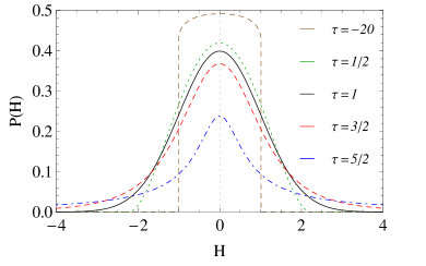
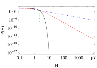
Figure 1: (Color online) Random-field probability distributions for some values of the parameter $\tau$ (from botton to top: $\tau=5/2,3/2,1,1/2$ and $-20$), in the normal (left panel) and log-log scale (right panel). We have used $\omega=1$ in all cases.

To boot, the functional form (3) is an asymptotic power-law decaying PDF with finite standard deviation for $1<\tau<5/3$ and an asymptotic power-law decaying PDF, but with infinite standard deviation instead. In both cases the decay exponent is equal to $2/(\tau-1)$. The latter case is also capable of reproducing the tail behavior of $\alpha$-stable Lévy distributions

$$\mathcal{L}_{\alpha}\left(H\right)=\int_{-\infty}^{\infty}\exp\left[-a\,\left|k\right|^{\alpha}+i\,k\,H\right]\,dk,$$

with $\alpha=\left(3-\tau\right)/\left(\tau-1\right)$ and broadness $a$, whose escort-distribution has got a finite width as well. For the case of the Cauchy-Lorentz, $\alpha=1$ ($\tau=2$) [the only case for which Lévy distributions are explicitly defined in real space], the parameter $a$ is equal to width $\omega$. Accordingly, if we bear in mind the previous work by Aharony aharony , we can hold that our enquiry also sheds light on the low temperature behavior of the random-field Ising model with the local magnetic field associated with a $\alpha$-stable Lévy distribution. In Fig. 1, we depict PDFs (2) and (3) for some values of $\tau$. Regarding the kurtosis,

$$\kappa\equiv\frac{\left\langle H^{4}\right\rangle}{\left\langle H^{2}\right\rangle^{2}},$$ (6)

the distribution is platykurtic, $\kappa<3$, for $\tau<1$ or leptokurtic, $\kappa>3$, for $\tau>1$. At this point it is important to stress that, as it has been made until now, in spite of being able to present non-mesokurtic distributions the combination of Gaussians results in asymptotic scale-dependent distributions.

From the free energy, $F(\{H_{i}\})$, associated with a given realization of site fields, $\{H_{i}\}$, we calculate the quenched average, $[F(\{H_{i}\})]_{H}$,

$$[F(\{H_{i}\})]_{H}=\int\prod_{i}[dH_{i}P(H_{i})]F(\{H_{i}\})~{}.$$ (7)

The general mean field result of the free energy per spin, in terms of any PDF of the random fields, is well-known schneiderpytte ; aharony , and is given by

$$f=\frac{J^{2}}{2}m^{2}-\frac{1}{\beta}\langle\,\log[2\cosh\beta(Jm+H)]\rangle_{H}$$ (8)

and the magnetization is given by,

$$m=\langle\,\mathrm{tanh}[\beta(Jm+H)]\rangle_{H},$$ (9)

where $\langle\,\ldots\rangle_{H}$ stands for averages over realizations of the disorder, i.e.,

$$\langle\,...\rangle_{H}=\int_{-\infty}^{+\infty}dH\;P(H)\;(...)~{}.$$

Close to a continuous transition between ordered and disordered phases, the magnetization $m$ is small. So, we can expand Eq. (9) in powers of $m$,

$$m=Am+Bm^{3}+Cm^{5}+\mathcal{O}(m^{7}),$$ (10)

where the coefficients are given by

$$A = \beta J\{1-\rho_{1}\},$$ (11)

$$B = -\frac{(\beta J)^{3}}{3}\{1-4\rho_{1}+3\rho_{2}\},$$ (12)

$$C = \frac{(\beta J)^{5}}{15}\{2-17\rho_{1}+30\rho_{2}-15\rho_{3}\},$$ (13)

with

$$\rho_{k}=\langle\,\tanh^{2k}(\beta H)\rangle_{H}~{}.$$

With the aim of finding the continuous critical frontier we set $A=1$, provided that $B<0$. If a first-order critical frontier also occurs, the continuous line must end when $B=0$; in such cases, the continuous and the first-order critical frontiers converge at a tricritical point, whose coordinates are obtained by solving the equations $A=1$ and $B=0$, on condition that $C<0$. Thus, for $A=1$, we obtain

$$\frac{kT}{J}=1-\langle\,\tanh^{2}(\beta H)\rangle_{H}~{}.$$ (14)

In the following section, we discuss the role of PDFs (2) and (3) when they are considered in the formulae presented in this section. Our survey includes the analysis of the phase diagrams for the whole domain of $\tau$.

III Finite Temperature Analysis

Following the above presented results, we proceed by calculating the critical frontiers of the model when the temperature is different from zero. In the RFIM, we have a single transition between the two possible phases of the magnetization: the ferromagnetic phase ($m\neq 0$) and the paramagnetic phase ($m=0$). The critical frontier separating these two phases is found by solving Eq. (14). On account of the fact that Eq. (14) is analytically unsolvable, we have been compelled to solve it by numerical means using the Global Adaptative Strategy algorithm kromer that has been proven as the best (i.e., fast and accurate) numerical integration procedure for smooth integrands malcom .

III.1 Platykurtic case: $\tau<1$

Let us denote $f_{i}$ and $m_{i}$ as the free energy and the magnetization for this regime of $\tau$, respectively. Thus, Eqs. (8) and (9) become,

$$f_{i}=\frac{J^{2}}{2}m_{i}^{2}-\frac{1}{\beta}\int_{-\frac{1}{\sqrt{\mathcal{B}_{\tau}(1-\tau)}}}^{\frac{1}{\sqrt{\mathcal{B}_{\tau}(1-\tau)}}}dH\,\,P_{i}(H)\log[2\cosh\beta(Jm_{i}+H)],$$ (15)

and

$$m_{i}=\int_{-\frac{1}{\sqrt{\mathcal{B}_{\tau}(1-\tau)}}}^{\frac{1}{\sqrt{\mathcal{B}_{\tau}(1-\tau)}}}P_{i}(H)\tanh\beta(Jm_{i}+H)~{},$$ (16)

where $P_{i}(H)$ is given by the PDF in Eq. (2). The continuous critical frontier has been found when we have solved Eq. (14). For all solutions obtained, we have calculated a negative value of $B$, Eq. (12), which has confirmed the continuous character of the phase transition.

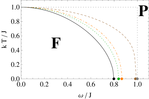
Figure 2: (Color online) Phase diagram of the model, in the plane temperature vs $\omega$ (in units of $J$), for some values of the parameter $\tau<1$. The grey dotted line is for $\tau=-\infty$  and $\omega\left(T=0\right)=J$; the brown dashed line is for $\tau=-20$ and $\omega\left(T=0\right)=0.9831\ldots J$; the dot-dashed orange line is for $\tau=0$ and $\omega\left(T=0\right)=0.8660\ldots J$; the dotted green line is for $\tau=1/2$ and $\omega\left(T=0\right)=3\sqrt{5/64}J$ and the black full line is the Gaussian case with $\omega\left(T=0\right)=\sqrt{2/\pi}J$. We can observe continuous phase transitions between the Ferromagnetic (F) and the Paramagnetic (P) phases for all values of $\tau$. The points onto the $\omega/J$ axis were exactly calculated through a zero-temperature analysis [section IV.A] where from we can see a good agreement between the analytical and numerical results which by interpolation indicates discrepancies never greater than 1%.

If a first-order transition existed as well, the critical frontier would be found by equalizing the free energy at each side of this line, i.e., $f(m=0)=f(m\neq 0)$. Using this procedure, we have numerically determined the critical frontiers separating the paramagnetic and ferromagnetic phases, for typical values of $\tau<1$. We have confirmed that the above coefficient $B$, Eq. (12), is always negative. The phase diagram is shown in Fig. 2, on the plane defined by the temperature, $T$, and the PDF width, $\omega$ (both in units of $J$), for some typical values of $\tau<1$. In that figure, the lines represent the numerical solution of Eq. (14), whereas the points were analytically obtained through a zero-temperature analysis, which is going to be discussed in the next section. Notice that the ferromagnetic phase is reduced by increasing the parameter $\tau$ from $\tau=-\infty$ to $\tau=1$ as shown in Fig. 2, and for the maximum value for $r$-distributions, $\tau=1$, we recover the simple phase diagram of the Gaussian distribution schneiderpytte .

III.2 Leptokurtic case: $\tau>1$

Analogously to the platykurtic case, we denote $f_{s}$ and $m_{s}$ as the free energy and the magnetization per spin for this regime of $\tau$. The expansion of the magnetization Eq. (10) is valid for this case as well, but the averages over the disorder $\langle\,\ldots\rangle_{H}$ must be made according to PDF (3),

$$f_{s} = \frac{J^{2}}{2}m_{s}^{2}-\frac{1}{\beta}\int_{-\infty}^{+\infty}dH\,\,P_{s}(H)\log[2\cosh\beta(Jm_{s}+H)],$$ (17)

$$m_{s} = \int_{-\infty}^{+\infty}P_{s}(H)\tanh\beta(Jm_{s}+H)~{},$$ (18)

where in this case the integration limits are taken in the range $(-\infty,+\infty)$.

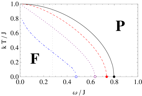
Figure 3: (Color online) Phase diagram of the model, in the plane temperature versus $\omega$ (in units of $J$), for some values of the parameter $\tau>1$. The black full line is the Gaussian case with $\omega\left(T=0\right)=\sqrt{\frac{2}{\pi}}J$; red dashed line is for $\tau=3/2$  and $\omega\left(T=0\right)=\frac{4}{\sqrt{3}\pi}J$; the purple dotted line is for $\tau=2$ and $\omega\left(T=0\right)=\frac{2}{\pi}J$; the dot-dashed blue line is for $\tau=5/2$ with $\omega\left(T=0\right)=0.4754\ldots J$. We can observe continuous phase transitions between the Ferromagnetic (F) and the Paramagnetic (P) phases for all values of $\tau$. The points represent the results obtained by the zero-temperature analysis. Notice the change in the concavity of the critical frontier for large values of $\tau$ ($>2.0$). The vertical dashed line is $\omega=0.275J$ which is close to the inflexion point of the critical line for $\tau=5/2$. In this figure, we have distinguished the points with finite free energy per spin from the points with a divergent free energy per spin representing the latter by empty circles. Again, we can observe a good agreement between the numerics and the expansion at $T=0$. The difference between the analytical approximation and interpolation is again never greater than 1%.

By considering PDF (3), the above presented procedure for the determination of the critical frontiers can be employed once more. In other words, Eq. (14) provide the continuous critical line of the phase diagram. Using this procedure, we have numerically evaluated the critical frontiers separating the paramagnetic and ferromagnetic phases for typical values of $\tau>1$. Like the platykurtic case, the leptokurtic case has only given negative values of $B$, $i.e.$, no other than continuous phase transition occurs. The phase diagram is shown in Fig. 3, on the plane formed by the temperature and the PDF width $\omega$ (in units of $J$), for some specific values of $\tau>1$. Still, the lines represent numerical solutions of Eq. (14), while at the same time the points were analytically obtained through a zero-temperature analysis, which is going to be discussed shortly. As we have perceived in the platykurtic case, the ferromagnetic phase is reduced by augmenting $\tau$. Similar behavior was found in the Gaussian schneiderpytte and the double-Gaussian RFIM nuno08 by increasing the standard deviation of such PDFs. However, a chief difference emerges. For distributions with fatter tails than the Cauchy-Lorentz PDF, the concavity of the critical frontier changes in the high-temperature region. So far as we are aware, this is the first time that such a change is observed in the mean-field RFIM phase diagram.

IV Zero Temperature Analysis

Moving forwards, we now consider the phase diagram of the model at zero temperature. As in the finite-temperature case, we evolve twofold: the platykurtic case and the leptokurtic case, $\tau<1$ and $\tau>1$, respectively.

IV.1 Platykurtic case: $\tau<1$

In the limit $T\rightarrow 0$, the free energy and magnetization become¹, respectively,

$$f_{i} = \frac{\Gamma\left[\frac{5-3\tau}{2\left(1-\tau\right)}\right]}{2(2-\tau)\Gamma\left[\frac{2-\tau}{1-\tau}\right]}\sqrt{\frac{1-\tau}{\left(5-3\tau\right)\pi}}$$ (19)

$$\left\{4\frac{(2-\tau)\,_{2}F_{1}\left[\frac{1}{2},\frac{1}{\tau-1};\frac{3}{2};\frac{\left(1-\tau\right)J^{2}}{(5-3\tau)\sigma^{2}}m_{i}^{2}\right]J^{2}}{\sigma}m_{i}^{2}+\right.$$

$$(5-3\tau)\sigma^{3}\left[2\left(1-\frac{(1-\tau)J^{2}}{(5-3\tau)\sigma^{4}}m_{i}^{2}\right)^{1+\frac{1}{1-\tau}}-1-\left[\sigma^{2}\left(\sigma^{2}-1\right)\right]^{{}^{1+\frac{1}{1-\tau}}}\right]+$$

$$\left.2(2-\tau)\sqrt{\frac{5-3\,\tau}{1-\tau}}\,_{2}F_{1}\left[\frac{1}{2},\frac{1}{\tau-1};\frac{3}{2};\frac{1}{\sigma^{2}}\right](1-J\,m_{i})\right\},$$

and

$$m_{i}=2\sqrt{\frac{1-\tau}{\left(5-3\tau\right)\pi}}\frac{\,\,\Gamma\left[\frac{5-3\tau}{2\left(1-\tau\right)}\right]}{\Gamma\left[\frac{2-\tau}{1-\tau}\right]}\left(\frac{J}{\sigma}\right)\,_{2}F_{1}\left[\frac{1}{2},\frac{1}{\tau-1};\frac{3}{2};\frac{(1-\tau)J^{2}}{(5-3\,\tau)\sigma^{2}}m_{i}^{2}\right]m_{i},$$ (20)

where ${}_{2}F_{1}[.,.;.;.]$ is the Gauss hypergeometric function hipergeometrica . In the same way as in the finite-temperature analysis, we expand the above magnetization (20) in powers of $m_{i}$, so that

$$m_{i}=a_{i}m_{i}+b_{i}m_{i}^{3}+c_{i}m_{i}^{5}+\mathcal{O}(m_{i}^{7}),$$ (21)

where

$$a_{i} = -2\left(\frac{J}{\sigma}\right)\sqrt{\frac{(1-\tau)^{3}}{(5-3\tau)\pi}}\frac{\Gamma\left[\frac{5-3\tau}{2\left(1-\tau\right)}\right]}{\Gamma\left[\frac{1}{1-\tau}\right]},$$ (22)

$$b_{i} = -\frac{2}{3\sqrt{\pi}}\left(\frac{J}{\sigma}\right)^{3}\left(\frac{1-\tau}{5-3\tau}\right)^{3/2}\frac{\Gamma\left[\frac{5-3\tau}{2\left(1-\tau\right)}\right]}{\Gamma\left[\frac{1}{1-\tau}\right]},$$ (23)

$$c_{i} = \frac{1}{5\sqrt{\pi}}\left(\frac{J}{\sigma}\right)^{5}\sqrt{\frac{1-\tau}{(5-3\tau)^{5}}\tau}\frac{\Gamma\left[\frac{5-3q}{2\left(1-q\right)}\right]}{\Gamma\left[\frac{2-\tau}{1-\tau}\right]}.$$ (24)

The continuous critical frontier at zero temperature is obtained for $a_{i}=1$,

$$\frac{\sigma}{J}=\frac{2(1-\tau)}{\sqrt{\pi}}\left(\frac{1-\tau}{5-3\tau}\right)^{1/2}\frac{\Gamma\left[\frac{5-3\tau}{2(1-\tau)}\right]}{\Gamma\left[\frac{1}{1-\tau}\right]},$$ (25)

providing that $b_{i}<0$, which occurs for all $\tau<1$. The last-mentioned equation allows determining the exact point at which the critical frontiers obtained in section 3.A reach the zero-temperature axis (the circles in Fig. 2). The zero-temperature phase diagram is shown in Fig. 4.

IV.2 Leptokurtic case: $\tau>1$

In this regime, PDF (3) presents a distinct behavior for $1<\tau<5/3$ and $\tau>5/3$. Explicitly, the former case corresponds to the case in which the standard deviation is finite and the latter to the case for which the distribution has the same asymptotic behavior as the Lévy distribution.

IV.2.1 Finite standard deviation: $1<\tau<5/3$

For this range of $\tau$, the free energy and the magnetization become,

$$f_{s} = \sqrt{\frac{5-3\tau}{\left(\tau-1\right)\pi}}\,\frac{\Gamma\left[\frac{2-\tau}{\tau-1}\right]}{\Gamma\left[\frac{3-\tau}{2\left(\tau-1\right)}\right]}\,\sigma\left\{\left[1-\frac{1-\tau}{5-3\tau}\left(\frac{J}{\sigma}\right)^{2}m_{s}^{2}\right]^{\frac{1}{1-\tau}+1}+\right.$$ (26)

$$\left.2(2-\tau)\left(\frac{J}{\sigma}\right)^{2}\,_{2}F_{1}\left[\frac{1}{2},\frac{1}{\tau-1};\frac{3}{2};-\frac{1-\tau}{5-3\tau}\left(\frac{J}{\sigma}\right)^{2}m_{s}^{2}\right]m_{s}^{2}\right\},$$

and

$$m_{s} = 2\,m_{s}\left(\frac{J}{\sigma}\right)\sqrt{\frac{\tau-1}{\left(5-3\tau\right)\pi}}\frac{\Gamma\left[\frac{1}{\tau-1}\right]}{\Gamma\left[\frac{3-\tau}{2\left(\tau-1\right)}\right]}\;\times$$

$${}_{2}F_{1}\left[\frac{1}{2},\frac{1}{\tau-1};\frac{3}{2};-\frac{1-\tau}{5-3\tau}\left(\frac{J}{\sigma}\right)^{2}m_{s}^{2}\right]~{},$$

respectively. Similarly to the $\tau<1$ analysis, we can expand the magnetization $m_{s}$, Eq. (IV.2.1), in powers of $m_{s}$,

$$m_{s}=a_{s}m_{s}+b_{s}m_{s}^{3}+c_{s}m_{s}^{5}+\mathcal{O}(m_{s}^{7}),$$ (28)

where,

$$a_{s} = 2\,\left(\frac{J}{\sigma}\right)\sqrt{\frac{\tau-1}{\left(5-3\tau\right)\pi}}\frac{\Gamma\left[\frac{1}{\tau-1}\right]}{\Gamma\left[\frac{3-\tau}{2\left(\tau-1\right)}\right]},$$ (29)

$$b_{s} = -\frac{4}{3}\left(\frac{J}{\sigma}\right)^{3}\sqrt{\frac{\left(\tau-1\right)^{3}}{\left(5-3\tau\right)^{5}\pi}}\frac{\Gamma\left[\frac{1}{\tau-1}\right]}{\Gamma\left[\frac{5-3\tau}{2\left(\tau-1\right)}\right]},$$ (30)

$$c_{s} = \left(\frac{J}{\sigma}\right)^{5}\frac{\tau}{5}\sqrt{\frac{\tau-1}{\left(5-3\tau\right)^{5}\pi}}\frac{\Gamma\left[\frac{1}{\tau-1}\right]}{\Gamma\left[\frac{3-\tau}{2\left(\tau-1\right)}\right]}.$$ (31)

The continuous critical frontier at zero temperature is obtained for $a_{s}=1$,

$$\frac{\sigma}{J}=\frac{2}{\sqrt{\pi}}\sqrt{\frac{\tau-1}{\left(5-3\tau\right)}}\frac{\Gamma\left[\frac{1}{\tau-1}\right]}{\Gamma\left[\frac{3-\tau}{2\left(\tau-1\right)}\right]}~{},$$ (32)

as long as $b_{s}<0$. In the range $1<\tau<5/3$, we notice that the coefficient $b_{s}$ is always negative, indicating the occurrence of continuous phase transitions for all values of $\tau$. This expression permit us to determine the values of $\sigma/J$, or equivalently, the values of $\omega/J$ [see Eq. (5)] at $T=0$ of the phase diagrams depicted in Fig. 3. In Fig. 4, we show the zero-temperature phase diagram, on the plane $\omega/J$ vs $\tau$.

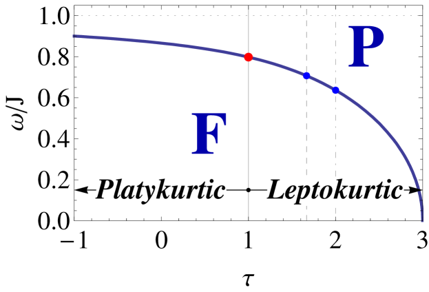
Figure 4: (Color online) Zero-temperature phase diagram separating the Ferromagnetic (F) and the Paramagnetic (P) phases for platykurtic ($\tau<1$) and leptokurtic ($\tau>1$) distributions. The horizontal dotted line represents the limiting case $\tau\rightarrow-\infty$, i.e., the uniform distribution ($\omega/J=1$), the dashed vertical line represents the limit for finite standard deviation ($\tau=5/3$) and the dot-dashed line the limit for finite average ($\tau=2$). The points emphasize the intersection between vertical lines and the critical line. They correspond to values of $\omega/J$ equal to $\sqrt{2/\pi}$, $1/\sqrt{2}$ and $2/\pi$, respectively.

IV.2.2 Finite width: $5/3<\tau<3$

Mark that in this range we must use $\omega$. Thus, as previously, the free energy and magnetization are respectively,

$$f_{s} = \sqrt{\frac{\tau-1}{\left(3-\tau\right)\pi}}\frac{\Gamma\left[\frac{1}{\tau-1}\right]}{\Gamma\left[\frac{3-\tau}{2\left(\tau-1\right)}\right]}\,\omega\,\left\{\frac{(3-\tau)}{(2-\tau)}\left(1-\frac{1-\tau}{3-\tau}\left(\frac{J}{\omega}\right)^{2}m_{s}^{2}\right)^{\frac{1}{1-\tau}+1}+\right.$$ (33)

$$\left.2\left(\frac{J}{\omega}\right)^{2}\,_{2}F_{1}\left(\frac{1}{2},\frac{1}{\tau-1};\frac{3}{2};-\frac{1-\tau}{3-\tau}\left(\frac{J}{\omega}\right)^{2}m_{s}^{2}\right)m_{s}^{2}\right\},$$

and

$$m_{s}=2\,m_{s}\left(\frac{J}{\omega}\right)\sqrt{\frac{\tau-1}{\left(3-\tau\right)\pi}}\frac{\Gamma\left[\frac{1}{\tau-1}\right]}{\Gamma\left[\frac{3-\tau}{2\left(\tau-1\right)}\right]}\;_{2}F_{1}\left[\frac{1}{2},\frac{1}{\tau-1};\frac{3}{2};\frac{\left(\tau-1\right)J^{2}}{\left(\tau-3\right)\omega^{2}}m_{s}^{2}\right].$$ (34)

Analogously to the above cases, we expand the magnetization $m_{s}$, Eq. (34), in powers of $m_{s}$,

$$m_{s}=a_{s}m_{s}+b_{s}m_{s}^{3}+c_{s}m_{s}^{5}+\mathcal{O}(m_{s}^{7}),$$ (35)

with the coefficients,

$$a_{s} = 2\left(\frac{J}{\omega}\right)\sqrt{\frac{\tau-1}{\left(3-\tau\right)\pi}}\frac{\Gamma\left[\frac{1}{\tau-1}\right]}{\Gamma\left[\frac{3-\tau}{2\left(\tau-1\right)}\right]},$$ (36)

$$b_{s} = -\frac{2}{3}\left(\frac{J}{\omega}\right)^{3}\sqrt{\frac{1}{\pi\left[(4-\tau)\tau-3\right]}}\frac{\Gamma\left[\frac{1}{\tau-1}\right]}{\Gamma\left[\frac{3-\tau}{2\left(\tau-1\right)}\right]},$$ (37)

$$c_{s} = \frac{2}{45}\left(\frac{J}{\omega}\right)^{5}\sqrt{\frac{\tau-1}{\left(3-\tau\right)\pi}}\frac{(5+9\tau)}{(3-\tau)^{2}}\frac{\Gamma\left[\frac{1}{\tau-1}\right]}{\Gamma\left[\frac{3-\tau}{2\left(\tau-1\right)}\right]},$$ (38)

Thus, the continuous critical frontier is given by

$$\frac{\omega}{J}=\frac{2}{\sqrt{\pi}}\left(\frac{\tau-1}{3-\tau}\right)^{1/2}\frac{\Gamma\left[\frac{1}{\tau-1}\right]}{\Gamma\left[\frac{3-\tau}{2(\tau-1)}\right]}~{},$$ (39)

and we have again verified that $b_{s}<0$ for all values $5/3<\tau<3$. We can see in Fig. 4 the zero-temperature phase diagram in the plane containing the width $\omega$ and the generalized degree of freedom $\tau$.

In this case, it is worth noticing an important result. In the free energy per spin (33), the integrals are finite only for $\tau<2$, i.e., the free energy at temperature equal to zero is not finite for probability density functions broader than the Cauchy-Lorentz. Although we do not have an unequivocal physical account for this phenomenon, we introduce some insight into this result with the help of the statistical meaning of our distributions. As mentioned in section 2, for $\tau>1$, distribution (3) is understood as a generalization of Student-$t$ for real degrees of freedom according to the relation,

$$\tau=\frac{3+m}{1+m}.$$ (40)

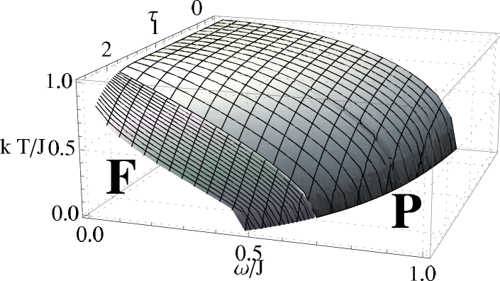
Figure 5: (Color online) Tri-dimensional phase diagram of the model in the axis temperature, $\tau$ and $\omega/J$, separating the Ferromagnetic (F) and the Paramagnetic (P) phases. We have used a darker color to represent the regime of $\tau$ ($\tau>2$) in which we have determined a divergent free energy per spin analytically found at $T=0$.

The Cauchy-Lorentz distribution, Eq. (3) with $\tau=2$, corresponds to the case for which the distribution presents a divergence in the average but a null average value of the corresponding escort distribution. The divergence of the mean value of the free energy for $\tau>2$ emerges from that feature of the property of Eq. (3). Moreover, this divergence was experimentally observed in organic charge-transfer compounds fat-materials .

In order to summarize the results presented in the manuscript, we show in Fig. 5 a tridimensional phase diagram separating the ferromagnetic (F) and the paramagnetic (P) phases defined by the axis temperature (in units of $J$), $\tau$ and $\omega$ (also in unit of $J$). We observe a contraction of the ferromagnetic phase for increasing values of $\tau$. We have spotted the above-described change in the concavity of the critical frontier for $\tau>2$, as well as the dwindling of the ferromagnetic phase (for increasing values of $\tau$) which in limit $\tau\rightarrow 3$ turns into the point $\omega=0$.

V Concluding remarks

In this work we have investigated the infinite-range-interaction Ising model in the presence of a random magnetic field following a family of continuous probability density functions, defined by a parameter $\tau$ comprising the $r$-distribution, for $\tau<1$, and the Student-$t,$ for $\tau>1$, which have already found their statistical relevance within other contexts of disordered systems. Moreover, specific PDFs like the Gaussian ($\tau\rightarrow 1$), the uniform ($\tau\rightarrow-\infty$) and the Cauchy-Lorentz ($\tau=2$) are obtained thereof. Independently of $\tau$, we have observed a continuous phase transition with the lessening of the ferromagnetic phase in the $\frac{k\,T}{J}$ vs $\frac{\omega}{J}$ plane that corresponds to the region defined by $0\leq\frac{k\,T}{J}\leq 1$ and $0\leq\frac{\omega}{J}\leq 1$ in the uniform case and to the point $\frac{\omega}{J}=\frac{k\,T}{J}=0$ for $\tau\rightarrow 3$. For $\tau\geq 2$, we have noted the appearance of an inflexion point for finite $\frac{\omega}{J}$ and $\frac{k\,T}{J}$ that is also associated with a divergence of the free energy per spin at null temperature for which we have provided with an explanation based on the statistical nature of distributions that are fatter than the Cauchy-Lorentz.

As an extension of this work, a numerical study by means of Monte Carlo simulations of the model defined by Eqs. (1), (2) and (3) in the case of nearest-neighbors interactions is though to bring a better understanding of the physical properties of the Ising model in the presence of random magnetic fields that follow continuous probability distributions part2 .

Acknowledgments

The authors acknowledge F. D. Nobre for discussions on several aspects of disordered magnetic systems. SMDQ benefits from financial support from the European Union’s Marie Curie Fellowship Programme and NC and DOSP thank the financial support from the Brazilian agency CNPq.

References

- (1) K. Binder and A. P. Young, Rev. Mod. Phys. 58, 801 (1986).
- (2) V. Dotsenko, Introduction to the Replica Theory of Disordered Statistical Systems (Cambridge University Press, Cambridge, 2001).
- (3) D. P. Belanger, in Spin Glasses and Random Fields, edited by A.P. Young (World Scientific, Singapore, 1998).
- (4) R.J. Birgeneau, J. Magn. Magn. Mater. 177, 1 (1998).
- (5) S. Fishman and A. Aharony, J. Phys. C 12, L729 (1979).
- (6) Po-Zen Wong, S. von Molnar and P. Dimon, J. Appl. Phys. 53 , 7954 (1982).
- (7) J. Cardy, Phys. Rev. B 29, 505 (1984).
- (8) J. Kushauer and W. Kleemann, J. Magn. Magn. Mater. 140–144 , 1551 (1995).
- (9) J. Machta, M.E.J. Newman and L.B. Chayes, Phys. Rev. E 62, 8782 (2000).
- (10) A.A. Middleton and D.S. Fisher, Phys. Rev. B 65, 134411 (2002).
- (11) A.K. Hartmann and A.P. Young, Phys. Rev. B 64, 214419 (2001).
- (12) M. Gofman, J. Adler, A. Aharony, A. B. Harris and M. Schwartz, Phys. Rev. B 53, 6362 (1996).
- (13) M.R. Swift, A.J. Bray, A. Maritan, M. Cieplak and J. R. Banavar, Europhys. Lett. 38, 273 (1997).
- (14) F. Wang and D. P. Landau, Phys. Rev. Lett. 86, 2050 (2001); Phys. Rev. E 64, 056101 (2001).
- (15) L. Hernández and H. Ceva, Phys. A 387, 2793 (2008).
- (16) Y. Wu and J. Machta, Phys. Rev. B 74, 064418 (2006).
- (17) T. Schneider and E. Pytte, Phys. Rev. B 15, 1519 (1977).
- (18) A. Aharony, Phys. Rev. B 18, 3318 (1978).
- (19) D.C. Mattis, Phys. Rev. Lett. 55, 3009 (1985).
- (20) M. Kaufman, P.E. Kluzinger and A. Khurana, Phys. Rev. B 34, 4766 (1986).
- (21) N. Crokidakis and F.D. Nobre, J. Phys. Condens. Matter 20, 145211 (2008).
- (22) O. R. Salmon, N. Crokidakis and F. D. Nobre, J. Phys. Condens. Matter 21, 056005 (2009).
- (23) A.T. Skjeltorp and T. Vicsek (Editors), Complexity from Microscopic to Macroscopic Scales: Coherence and Large Deviations (Kluwer Academic Publishers, Dordrecht, 2002)
- (24) G. Theodorou and M.H. Cohen, Phys. Rev. Lett. 37, 1014 (1976); G. Theodorou, Phys. Rev. B 16, 2264 (1977); C. Dasgupta and S. Ma, Phys. Rev. B 22, 1305 (1980).
- (25) J.C. Scott , A.F. Garito , A.J. Heeger , P. Nannelli and H.D. Gillman, Phys. Rev. B 12, 356 (1975).
- (26) Student, Biometrika 6, 1 (1908).
- (27) C. Tsallis, J. Stat. Phys. 52, 479 (1988).
- (28) A.M.C. de Souza and C. Tsallis, Phys. A 236, 52 (1997).
- (29) C. Beck and F. Schögl,Thermodynamics of Chaotic Systems: an introduction (Cambridge University Press, Cambridge, 1993)
- (30) H.J. Hilhorst, e-print arXiv:0901.1249v2 [cond-mat.stat-mech](preprint, 2009).
- (31) A.R. Krommer and C.W. Ueberhuber, Computational Integration (SIAM Publications, Philadelphia, 1998).
- (32) M.A. Malcolm and R.B. Simpson, ACM Trans. Math. Soft. 1, 129 (1975).
- (33) I.S. Gradshteyn and I.M. Ryzhik, Table of Integrals, Series, and Products (Academic Press, New York, 1980), sec. 3.19
- (34) http://functions.wolfram.com/HypergeometricFunctions/Hypergeometric2F1/
- (35) N. Crokidakis, D.O. Soares-Pinto and S.M. Duarte Queirós, in preparation.