Theory of vortex states in magnetic nanodisks with induced Dzyaloshinskii-Moriya interactions

Abstract

Vortex states in magnetic nanodisks are essentially affected by surface/interface induced Dzyaloshinskii-Moriya interactions. Within a micromagnetic approach we calculate the equilibrium sizes and shape of the vortices as functions of magnetic field, the material and geometrical parameters of nanodisks. It was found that the Dzyaloshinskii-Moriya coupling can considerably increase sizes of vortices with ”right” chirality and suppress vortices with opposite chirality. This allows to form a bistable system of homochiral vortices as a basic element for storage applications.

I Introduction

Physics of magnetism at nano- and submicrometer scales is an object of broad and intensive scientific investigations stimulated by various possible applications including magnetic random access memory, high-density magnetic recording media, and magnetic sensors.Prinz98 Nanoscale magnetic dots with vortex states are considered as promising components for such spintronic devices.Bussmann99 ; Zhu00 ; Bohlens08 Numerous experimental observations show that such vortices consist of a narrow core with a perpendicular magnetization surrounded by an extended area with in-plane magnetization curling around the center (Fig. 1). Shinjo00 ; Wachowiak02 ; Raabe00 ; Schneider00 ; Schneider01 It has been proposed to use both the up and down polarity, i.e. the perpendicular magnetization of a vortex, or the rotation sense of the curling in-plane magnetization as switchable bit elements in memory devices.Bussmann99 ; Zhu00 ; Bohlens08

The vortex state in thin film elements results from the necessity to reduce the demagnetization energy in competition with the exchange coupling.Feldtkeller65 ; Hubert In circular disks the axisymmetric ground state arises for diameters in the range of a few nanometer up to many 10 nm depending on magnetic material. For very small diameters, a single domain state occurs, very large film elements form multidomain states. Within the usual micromagnetic calculations the shape and size of the vortices are determined by the competition between exchange and stray field energy.Guslienko08 In particular, the vortices with different chirality are degenerate: the four possible vortex ground-states differentiated by their handedness and polarity all have the same energy within these standard micromagnetic models.

The broken inversion symmetry at the surface of magnetic films, however, induces chiral magnetic couplings in the form of Dzyaloshinskii-Moriya (DM) exchange as a result of relativistic spin-orbit interactions.Fert90 ; Crepieux98 ; PRL01 The chiral DM interactions destabilize collinear magnetic states and are able to create a large variety of helical and Skyrmionic spin textures.Dz64 ; ANB89 ; JMMM94 ; PRL01 ; Nature06 The mechanism and phenomenological models of the surface-induced DM couplings, along with possible observable effects in magnetic films, have been discussed earlier.Crepieux98 ; PRL01 These theories now are supported by modern quantitative ab initio calculations for magnetic nanostructures.Udvardi03 ; Heide06 ; Antal08 ; Mankovsky09 Recent experiments Bode07 ; Ferriani08 provide clear evidence for these surface-induced DM interactions, as they display long-period modulated non-collinear magnetic states, which can be identified as chiral Dzyaloshinskii spirals.Dz64 Chiral effects observed for magnetization processes in vortex states of magnetic nanodisks Curcic08 may also belong to this class of phenomena.

In this work, we describe the chiral symmetry breaking in the vortex ground states of circular thin film elements within a basic micromagnetic approach. As the vortex states are chiral themselves, the effect of the chiral DM is less obvious. However, in the presence of DM interactions the chiral degeneracy of the left- and right-handed vortices is lifted. The simplicity of the circular vortex structure makes them amenable to detailed theoretical investigations. Here, we calculate the differences between the core shapes and sizes of left- and right-handed vortices in the presence of DM couplings. These differences of core structure may be observable in experiments, e.g. as differences in core diameter or net polarity of vortices, when switching their chirality. We suggest that such experiments can be used to determine the magnitude of surface-induced DM couplings in ultrathin magnetic films/film elements.

II Equations and methods

The energy density of a uniaxial ferromagnet with chiral interactions can be written in the following form JMMM94

$$w = A\sum_{i,j}\left(\frac{\partial m_{j}}{\partial x_{i}}\right)^{2}-\mathbf{M}\cdot\mathbf{H}-\frac{1}{2}\mathbf{M}\cdot\mathbf{H}_{m}$$ (1)

$$+K_{u}(\mathbf{m}\cdot\mathbf{a})^{2}+w_{D},$$

where $\mathbf{m}$ is the unity vector along the magnetization $\mathbf{M}=M_{s}\mathbf{m}$ and $M_{s}$ is the saturation magnetization. The couplings are given by the exchange stiffness $A$.The anisotropy axis $\mathbf{a}$ is taken perpendicularly to the disk surface, and $K_{u}$ is the anisotropy constant which must be positive in easy-plane materials. $\mathbf{H}$ is the external magnetic field, and $\mathbf{H}_{m}$ is the stray field. The Dzyaloshinskii-Moriya energy $w_{D}$ is described by so-called Lifshitz invariants,Dz64 energy terms linear in first spatial derivativs of the magnetization,

$$L_{ij}^{(k)}=m_{i}\frac{\partial m_{j}}{\partial x_{k}}-m_{j}\frac{\partial m_{i}}{\partial x_{k}}\,.$$ (2)

The functional form of this energy is determined by the symmetry of the surface/interfaces.Crepieux98 In this paper we use $w_{D}$ terms in the following form

$$w_{D}=D\left(L_{zx}^{(y)}-L_{zy}^{(x)}\right)\,,$$ (3)

which gives the allowed Lifshitz invariants of the magnetization in symmetries from Laue classes 32, 42, and 62. This $w_{D}$ term favours the curling mode of the magnetization, where the rotation sense is determined by the sign of the Dzyaloshinskii constant $D$. Depending on crystallographic symmetry, other types of Lifshitz invariants may occur which may favour differently twisted non-collinear magnetization structures. For example, Lifshitz invariants $(L_{zx}^{(x)}+L_{zy}^{(y)})$, possible in Laue classes 3m, 4m, and 6m, induce a cycloidal rotation of the magnetization vector.JMMM94 The various possibilities can be deduced from the corresponding list of Lifshitz invariants for three-dimensional Laue classes in Ref.ANB89 , where also the structures of the corresponding Dzyaloshinskii spirals and circular vortex-like Skyrmions have been presented. For simplicity, we restrict discussion here to the form of Eq. (2).

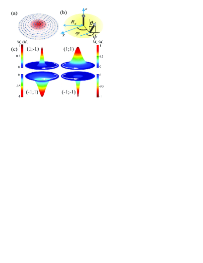
Figure 1: (a) Vortex states in a circular magnetic nanodisk of radius $R_{d}$ with axisymmetric magnetization structure. (b) Geometry and definition of variables of the problem. (c) The four possible vortex states are characterized by the indices (polarity $p=\pm 1$; chirality $c=\pm 1$) Dzyaloshinskii-Moriya couplings with chirality $\tilde{c}=1$ ($D>0$) widen vortices with the same chirality, $c=1$, and squeeze vortices with opposite chirality, $c=-1$.

The equilibrium configurations of $\mathbf{m}$ are derived by solving the equations minimizing the energy (1) together with equations of magnetostatics. To describe vortex states in a disk of radius $R_{d}$ and with zero or perpendicular applied field, we consider axisymmetric distributions of the magnetization and express the magnetization vector m in terms of spherical coordinates and the spatial variables in cylindrical coordinates: $\mathbf{m}=(\sin\theta\cos\psi;\sin\theta\sin\psi;\cos\theta)$, $\mathbf{r}=(\rho\cos\varphi;\rho\sin\varphi;z)$ (Fig. 1, b). The vortices are characterized by the magnetization direction in the center, polarity $p=\pm 1$, and the chirality of the magnetization structure, chirality $c=\pm 1$. Four different vortex states can be described by the indices ($p;c$) (Fig. 1, c). One can introduce the chirality of the Dzyaloshinskii-Moriya coupling as $D=|D|\tilde{c}$. Then the Dzyaloshinskii-Moriya interactions favours states with $c=\tilde{c}$ and suppresses those with opposite chirality $c=-\tilde{c}$. In this paper we assume for definiteness that the vortices have positive chirality, $c=1$, and study their properties for $D{{<}\atop{>}}\,0$. Thus, positive DM couplings favour these vortices, while they are suppressed in the opposite case, $D<0$.

Due to the non-local character of stray-field interactions the micromagnetic problem Eq. (1) constitutes a set of integro-differential equations.Hubert In order to simplify this problem we consider the limit of a thin film where the magnetodipole energy has a local character and reduces to a “shape” anisotropy $K_{m}=2\pi M_{s}^{2}$.Gioia97 This can be added to the uniaxial anisotropy $K_{u}$ yielding a redefinition of the anisotropy energy in Eq. (1) by an effective anisotropy constant $K$. We also introduce the characteristic (exchange) length $l_{e}$, the anisotropy field $H_{a}$, and a critical value of the Dzyaloshinskii constant $D_{0}$

$$l_{e}=\sqrt{A/K},\quad H_{a}=2K/M_{s},$$

$$D_{0}=\sqrt{AK},\quad K=K_{u}+2\pi M_{s}^{2}>0,$$ (4)

as proper material parameters of the problem. They establish important relations between vortex solutions and magnetic states in laterally infinite magnetic nanolayers. The anisotropy field determines the equilibrium magnetization of homogeneously magnetized layers in an applied perpendicular field $H$,

$$\cos\theta_{h}=H/H_{a}\,.$$ (5)

The constant $D_{0}$ gives a threshold ”strength” of the DM coupling in comparison with the exchange and anisotropy: for $|D|/D_{0}>4/\pi=1.273$ the magnetization of a layer transforms into a modulated state.Dz64 ; JMMM94 The exchange length gives a characteristic radius of the vortex core. Most experimentally investigated nanodisks have radii much larger than the exchange length, $R_{d}\gg l_{e}$. In this case vortices consist of a strongly localized core encircled by a wide ring with a constant polar angle $\theta=\theta_{h}$ (Fig. 1 (a)).

The variational problem for functional (1) has rotationally symmetric solutions $\psi=\varphi\pm\pi/2$, $\theta=\theta(\rho)$. By substituting the solution for $\psi$ into Eq. (1) and integrating with respect to $\varphi$ the vortex energy can be reduced to the following form $E=2\pi\int^{R_{d}}_{0}w(\rho)\rho d\rho$, where

$$w(\rho) = A\left[\left(\frac{d\theta}{d\rho}\right)^{2}+\frac{1}{\rho^{2}}\sin^{2}\theta\right]+K\cos^{2}\theta$$

$$- HM_{s}\cos\theta-D\left(\frac{d\theta}{d\rho}+\frac{1}{\rho}\cos\theta\sin\theta\right),$$

where the magnetic field $H$ is assumed to be perpendicular to the disk plane.

The Euler equation for $\theta(\rho)$

$$A\left(\frac{d^{2}\theta}{d\rho^{2}}+\frac{1}{\rho}\frac{d\theta}{d\rho}-\frac{1}{\rho^{2}}\sin\theta\cos\theta\right)-\frac{D}{\rho}\sin^{2}\theta$$

$$+K\sin\theta\cos\theta-HM_{s}\sin\theta/2=0$$ (7)

with the boundary conditions

$$\theta(0)=0,\,\quad\left(d\theta/d\rho\right)_{\rho=R_{d}}=g(\theta,R_{d})$$ (8)

yield the equilibrium vortex profiles. $g(\theta,R_{d})$ describes the anchoring effect imposed by the surface energy at the disk edge. For $D=H=g(\theta,R_{d})=0$ and infinite radius, Eq. (II) is related to the differential equation introduced by Ginzburg and Pitaevskii in their theory of superfluid vortices in liquid helium.Ginzburg58 Similar equations describe vortex excitations in different bosonic systems including Bose-Einstein condensates (see e.g. Feder99 ) and easy-plane magnets.Gouvea89

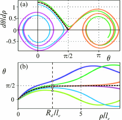
Figure 2: (a) Typical phase space trajectories for the solutions of the auxiliary Cauchy problem (Eqs. (II), (9)). (b) Corresponding profiles $\theta(\rho)$. The shown trajectories pertains to the case $H=0$, $\theta_{h}=\pi/2$. Due to the localized character of the vortex states the equilibrium solutions $\theta(\rho)$ of the boundary problem (II), (8) are close to the localized profiles given by the (dashed) separatrix lines in the phase portrait.

As a first step in solving the boundary value problem (Eqs. (II), (8)) we consider an auxiliary Cauchy problem for Eq. (II) with initial conditions

$$\theta(0)=0,\quad(d\theta/d\rho)_{\rho=0}=\alpha$$ (9)

for different values of $\alpha>0$. The trajectories $\theta(\rho;\alpha)$ for this initial value problem with $0<\alpha<\infty$ define a family of solutions parametrized by $\alpha$. Any solution $\theta(\rho)$ of the boundary problem (II), (8) is member of this family for a certain value of $\alpha$. A qualitative analysis of possible trajectories in the phase space, $d\theta/d\rho\equiv\theta_{\rho}$ vs. $\theta$, makes it possible to single out the desired solution among other trajectories. Typical trajectories $\theta_{\rho}(\theta)$ for the Cauchy problem are presented in the phase space portrait shown in Fig. 2. For arbitrary values of $\alpha$ the lines $\theta_{\rho}(\theta)$ usually end by spiraling around one of the attractors $(\pi n,0)$, $n=\pm 1,\pm 2\dots$. But for a certain value $\tilde{\alpha}$ the line $\theta_{\rho}(\theta)$ ends in the point $(\theta_{h},0)$. Thus, variation of parameter $0<\alpha<\infty$ (9) allows to select the solutions of the boundary problem (II), (8). The trajectories $\theta(\rho)$ have arrow-like shape. Their core sizes can be introduced in a manner commonly used for magnetic domain walls Hubert and Skyrmions JMMM94 : as the point $R_{0}$ where the tangent at the origin point intersects the line $\theta=\theta_{h}$,

$$R_{0}=\theta_{h}\left(d\theta/d\rho\right)^{-1}_{\rho=0}=\theta_{h}/\alpha.$$ (10)

The solution of the boundary value problem (II), (8) can be readily found from a set of solutions of the Cauchy problem $\theta(\rho;\alpha)$. Namely, the solution is given by the profile $\theta(\rho)$ which crosses line $\rho=R_{d}$ at the angle $\beta=\arctan(g(\theta,R_{d}))$ (Fig. 2 (b)). The family of the solutions $\theta(\rho;\alpha)$ of the Cauchy problem establishes the connections between the equilibrium vortex size ($R_{0}\propto 1/\alpha$), the disk radius $R_{d}$, and the anchoring energy $g(\theta,R_{d})$. The trajectories $\theta(\rho;\alpha)$ in Fig. 2 (b) visually demonstrate how the vortex core size depends on the disk radius $R_{d}$ and the boundary anchoring at the edges. This dependence should be noticeable in small disks with radii comparable to the exchange length $l_{e}$. In real magnetic nanodisks one usually has $R_{d}\gg l_{c}$.Shinjo00 In this case the solutions of Eqs. (II), (8) are very close to separatrix lines and the equilibrium core retains a fixed shape and size almost identical to the separatrix solution $\tilde{\alpha}$ and $\theta_{h}$, largely independent from the radius $R_{d}$ and the anchoring energy. In this connection see an interesting discussion on vortex core sizes in Ref. Li06 .

The independence of the core structure on boundary conditions allows to neglect effects imposed by the anchoring energy at the edges. Thus, we consider here the problem with free boundary conditions, $g(\theta,R_{d})=0$. Eqs. (II), (8) include two independent material parameters, $D/D_{0}$ and $H/H_{a}$. For fixed values of these control parameters the solutions of the vortex profile have been derived by using the following numerical procedure. The Cauchy problem (II), (9) was solved by the Runge-Kutta method. Through repeated calculations for varying values $\alpha$, the correct trajectory was searched by ’shooting’ at the boundary condition value (8). After that the profiles have been improved by a relaxation calculation using a finite-difference method for the boundary value problem, for details see Ref.JMMM94 .

The chirality of a non-collinear structure can be measured from the strength of the twist or helical rotation of the magnetization, $\mathbf{m}\cdot(\nabla\times\mathbf{m})$. For the radial vortex structure, the local twist is given by the expression

$$\tau=\left(\frac{d\theta}{d\rho}+\frac{1}{\rho}\cos\theta\sin\theta\right)\,.$$ (11)

The sign of this expression measures the local and helical chirality in the structure. The comparison with Eq. (II) shows that the local twist is equivalent to the local density of the DM energy. In particular, for $0\leq\theta\leq\pi/2$ and $\theta_{\rho}>0$ the local chirality of the helical structure is positive. Alternatively, the local chirality can be measured by the $\mu=z$ component of the chiral current $j_{\mu}=(1/(8\pi^{2})\epsilon_{\mu\nu\lambda}\mathbf{m}\cdot(\partial_{\nu}\mathbf{m}\times\partial_{\lambda}\mathbf{m})$. The evaluation for the vortices structure gives a chirality

$$\chi=(\theta_{\rho}/(2\pi\rho))\sin\theta\,.$$ (12)

Both the sign of $\tau$ and $\chi$ can be used to determine the local handedness in the vortex structure. In particular, a change of slope for the profile from $\theta_{\rho}>0$ to $\theta_{\rho}<0$ changes the chirality of the magnetization structure (Fig. 3, Inset).

III Results

In this section we present the results for the vortex core structures first from exact numerical calculations. Then an analytical ansatz is discussed which offers qualitative insight on the dependence and mechanism by which DM couplings influence the core structure of vortices. Finally the stability and static distortion modes of the vortex solutions are investigated.

III.1 Vortex solutions and magnetization profiles

Typical solutions of Eq. (II) for different values of $D$ in zero field are shown in Fig. 3. The effect of applied perpendicular fields on the core structure is demonstrated in Fig. 4. All reported results from the numerical solution of the boundary problem (II),(8) are for a fixed disk radius $R_{d}=30l_{e}$. As discussed, the solutions well represent the vortex core properties for any $R_{d}\gg l_{e}$.

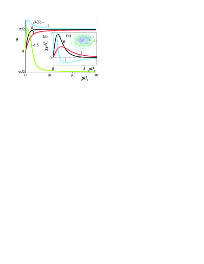
Figure 3: Typical solutions $\theta(\rho)$ for different values of $D$ in zero applied field. The vortices widen when their chirality $c=1$ coincides with the chirality of the DM interaction, $D>0$. In the opposite case, $D<0$, the vortex cores shrink, and the local chirality $\chi(\rho)$ changes its sign outside the vortex core (Inset a). The core with unfourable chirality is encircled by a ring with negative local polarization and favourable chirality (Inset b). For strong negative DM coupling ($D/D_{0}=-1.5$) the circulation of the projected magnetization in the plane changes the sense of rotation from positive in the core to negative at the edge, $\theta\rightarrow-\pi/2$ at $R_{d}$.

Vortex profiles $\theta(\rho)$ have an arrow-like shape. For $D>0$ the angles $\theta$ vary monotonically from zero at the vortex axis to $\theta_{h}$ (5). In this case the magnetization has everywhere a local chirality favoured by the Dzyaloshinskii-Moriya interactions. The core size widens with increasing $D$.

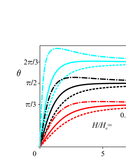
Figure 4: Typical solutions $\theta(\rho)$ for different values of the applied field and the reduced values of the Dzyaloshinskii constant: $D/D_{0}$ = 0 (solid lines), 0.5 (dashed lines), -0.5 (dash-dotted lines).

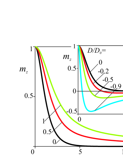
Figure 5: Magnetization profiles $m_{z}(\rho/l_{c})$ for different values of $D$. For $D>0$ the perpendicular magnetized central spot broadens with increasing D. For negative $D$ an increasing $|D|$ widens the ring with negative $m_{z}$ and compresses a central spot with positive $m_{z}$ (Inset).

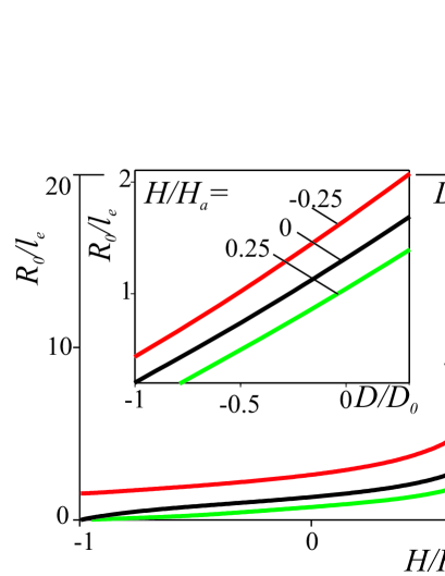
Figure 6: The equilibrium sizes of vortex core $R_{0}$ (10) as functions of reduced magnetic field $H/H_{a}$ for different values of $D/D_{0}$. Inset shows $R_{0}$ as functions of $D/D_{0}$ for different values of the applied magnetic fields.

For negative $D$ the magnetization in the core has unfavourable chirality. As a result in a certain point $\rho_{r}$ with $\theta(\rho_{r})>\theta_{h}$ the profile $\theta(\rho)$ goes through a maximum, $\theta>\pi/2$ in zero field, the slope $\theta_{\rho}$ becomes negative, and the magnetization structure changes its local chirality. After that, in the range $\rho_{r}<\rho<R_{d}$ the polar angle $\theta(\rho)$ monotonically approaches the limiting value $\theta_{h}$. As the magnitude of the negative $D$ increases these vortices transform into those with ”reverse” rotation to $-\theta_{h}$ (profile with $D=-1.5$ in Fig. 3). For $D<0$ the vortex core consists of a narrow internal part ($\rho<\rho_{r}$) and the adjacent ring with a reverse magnetization rotation.

Peculiarities of the vortex profiles for different sign of $D$ are reflected in their magnetization distribution (Fig. 5). Positive $D$ increases the width of the central spot with $m_{z}>0$ (Fig. 5). As a result the total perpendicular magnetization of the disk $<m_{z}>=\int_{0}^{R_{d}}m_{z}(\rho)\rho d\rho$ is larger in vortices of the right positive chirality. Negative $D$ squeezes the central magnetization core with $m_{z}>0$ and widens the adjacent ring with negative perpendicular magnetization ($m_{z}<0$) (Fig. 5, Inset). The overall behavior of the vortex core sizes is summarized in Fig. 6 by displaying the dependence of the core radii $R_{0}$, as defined in Eq. (10), on the external field for different zero, positive, and negative values of $D$. This dependence is weak and almost linear up to large fields $H/H_{a}\rightarrow 1$, where the transition into the homogeneously magnetized state takes place. The Inset of Fig. 6 shows that the dependence of $R_{0}$ on $D$ is almost linear both for zero field and for not too large positive and negative fields.

III.2 Linear ansatz and analytical results for a vortex core

Vortex profiles with strongly localized arrow-like cores (Fig. 3) can be described by a linear ansatz for the core and a flat part,

$$\theta=\theta_{h}(\rho/R),\quad 0<\rho<R,$$

$$\theta=\theta_{h},\quad R<\rho<R_{d}.$$ (13)

Integration of the energy functional Eq. (II) with the ansatz $\theta(\rho)$ (13) leads to the following expression for the vortex energy as a function of $R$,

$$\mathcal{E}(R)=\mathcal{K}R^{2}-\mathcal{A}\ln R-\tilde{c}\mathcal{D}R\,,$$ (14)

where $\mathcal{K}=\pi g_{0}(H)K$, $\mathcal{D}=4\pi g_{1}(H)D$, $\mathcal{A}=2\pi g_{2}(H)A$, and $g_{0}(H)=(\theta_{h}^{2}(1+2\cos^{2}\theta_{h})-3\theta_{h}\sin 2\theta_{h}-7\cos^{2}\theta_{h}+8\cos\theta_{h}-1)/(2\theta_{h}^{2})$, $g_{1}(H)=(\sin^{2}\theta_{h}-\theta_{h}\sin 2\theta_{h}+\theta^{2}_{h})/(4\theta_{h})$, $g_{2}(H)=\sin^{2}\theta_{h}$, and $\theta_{h}$ is the solution of Eq. (5). In Eq. (14) we omit terms independent on parameter $R$. Minimization of energy (14) yields the equilibrium radii of the core for positive and negative $D$

$$R_{1,2}=u(H)l_{e}\left[\sqrt{\left(\frac{D}{D_{0}}\right)^{2}+v^{2}(H)}+\tilde{c}\frac{|D|}{D_{0}}\right],$$ (15)

where $u(H)=g_{1}(H)/g_{0}(H)$, $v(H)=\sqrt{g_{0}(H)g_{2}(H)}/g_{1}(H)$. Particularly, at zero field $u(0)=1.856,v(0)=0.988$.

Eqs. (14), (15) offer an important insight into the physical mechanism that underlies the formation of the vortex states. The exchange energy of the vortex core does not depend on its size. This reflects a general property of vortex and 2D Skyrmionic states.Derrick64 ; Nature06 The exchange energy of the adjacent ring ($\propto-A\ln R$) favours the extension of the vortex cores while the magnetic anisotropy energy $\propto KR^{2}$ tends to compress them. For $D=0$ the balance between these energy contributions yields the equilibrium core sizes $R\propto\sqrt{A/K}$, equal for the vortices of opposite chirality. Finite values of $D$ violate chiral symmetry of the solutions (15) stabilizing vortices with different sizes of the core. The difference between core sizes in vortices with different chirality can be readily derived from Eq. (15),

$$\Delta R=|R_{1}-R_{2}|=2l_{e}\frac{|D|}{D_{0}}u(H)\,.$$ (16)

The numerical calculations of $\Delta R$ also reveal a linear relation $\Delta R=a(D/D_{0})$, where the coefficient $a$ depends on the applied field. Particularly $a(H/Ha)$ has the following values: $a(0)=2.4$, $a(0.25)=2.66$, and $a(-0.25)=2.24$.

III.3 Radial stability of the solutions

To study radial stability of vortices we consider a small arbitrary radial distortion $\xi(\rho)$ of the solutions $\theta(\rho)$ of Eqs. (II), (8) with the boundary conditions $\xi(0)=\xi(R_{d})=0$. We insert $\tilde{\theta}(\rho)=\theta(\rho)+\xi(\rho)$ into energy functional Eq. (II) and keep only terms up to second order in $\xi(\rho)$. Because $\theta(\rho)$ is the solution of the boundary value problem the first-order term must vanish, and one obtains $E=E^{(0)}+E^{(2)}$ where $E^{(0)}$ is the equilibrium energy, and

$$E^{(2)}=2\pi\int^{R}_{0}\left[A\left(\frac{d\xi}{d\rho}\right)^{2}+G(\rho)\xi^{2}\right]\rho\,d\rho$$ (17)

with

$$G(\rho) = \frac{A}{\rho^{2}}\cos 2\theta-K\cos 2\theta$$

$$+\frac{1}{2}HM_{s}\cos\theta+\frac{D}{\rho}\sin 2\theta\,.$$

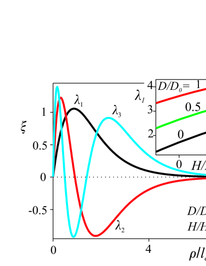
Figure 7: The first three excitation modes for $D/D_{0}=0.5$ and $H/H_{a}=0.25$ and corresponding eigenvalues: $\lambda_{1}=2.966$, $\lambda_{2}=8.428$, $\lambda_{3}=15.685$. The structure is radially stable because the smallest eigenvalue $\lambda_{1}$ is positive. Inset shows the first eigenvalue as a function of the applied field and for different values of $D/D_{0}$.

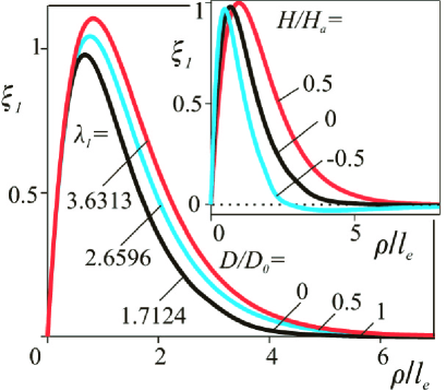
Figure 8: The first excitation mode $\xi_{1}(\rho)$ at zero field and for different values of the Dzyaloshinskii constant. Inset shows $\xi_{1}(\rho)$ for $D=0$ and different values of the applied field. Corresponding eigenvalues $\lambda_{1}(H/H_{a})$: $\lambda_{1}(-0.5)=0.9556$, $\lambda_{1}(0)=1.7124$, $\lambda_{1}(0.5)=2.3644$.

The stability problem is reduced to the solution of the spectral problem for functional (17) (for details see Ref. JMMM94 ). By expanding $\xi(\rho)$ in a Fourier series

$$\xi(\rho)=\sum^{\infty}_{k=1}b_{k}\sin(ak\theta(\rho)),$$ (19)

where $a=\pi/\theta_{h}$ the perturbation energy $E^{(2)}$(17) can be reduced to the following quadratic form

$$E^{(2)}=\sum^{\infty}_{k,j=1}A_{kj}b_{k}b_{j}$$ (20)

with

$$A_{kj}=\int^{R}_{0}[Aa^{2}kj\cos(ak\theta)\cos(aj\theta)+$$ (21)

$$+G(\rho)\sin(ak\theta)\sin(aj\theta)]\rho d\rho.$$

Radial stability of the solution is determined by the sign of the smallest eigenvalue $\lambda_{1}$ of matrix A: if $\lambda_{1}>0$ the solution $\theta(\rho)$ is stable with respect to perturbations $\xi(\rho)$, and the solutions are radially unstable if $\lambda_{1}$ is negative.

Numerical calculations demonstrate radial stability of vortex solutions for positive $D$ in the whole range of the magnetic fields where these solutions exist. For $H=0.25$, $D=0.5$ the first three excitation modes $\xi(\rho)$ and their eigenvalues are shown in Fig. 7. The variation of the first eigenfunctions and eigenvalues under the influence of the applied field and $D>0$ is shown in Fig. 8. The lowest perturbation eigenfunctions are connected with an expansion or compression of the vortices. The eigenvalues and the eigenfunctions correspond to certain magnetic resonance modes associated with radial deformations of the vortex core.

For $D<0$ radial stable solutions exist only below certain critical strength of the Dzyaloshinskii constant $|D|<|D_{cr}|$. For $|D|>|D_{cr}|$ vortex solutions are radially unstable. Detailed investigations of vortex structures for $D<0$ beyond this threshold and their stability is beyond this contribution restricted to axisymmetric simple vortex structures.

IV Conclusions

We have investigated the influence of induced Dzyaloshinskii-Moriya interactions on the equilibrium vortex parameters in magnetic nanodisks. Both numerical and analytical calculations demonstrate strong dependencies of the vortex structures (Fig. 3), magnetization profiles (Fig. 5), and core sizes (Fig. 6) on the strength and sign of the Dzyaloshinskii-Moriya coupling. Thus, by switching the chirality of a vortex a change of the vortex profile, core size, and the perpendicular magnetization takes place in the presence of a surface-induced Dzyaloshinskii-Moriya coupling. Existing experimental imaging techniques should already be sufficient to investigate these differences in vortex states with different chirality.Raabe00 ; Schneider00 ; Schneider01 ; Curcic08 ; Shinjo00 ; Wachowiak02 ; Li06 ; Tanase09 ; Weigand09 ; Loubens08 The calculated relations between strength of the Dzyaloshinskii-Moriya interactions and vortex core sizes (Fig. 6 and Eqs. (15), (16)) provide a method for experimental determination of the Dzyaloshinskii constant $D$.

From the theoretical side our results obtained within a simplified micromagnetic model can be extended. The calculated dependence of the excitation modes in Fig. 7 on the Dzyaloshinskii-Moriya interactions indicate that magnetic resonances of vortex cores, or more generally dynamical effects, may provide a route to investigate chiral symmetry breaking in film elements with vortex states. Many recent experimental Tanase09 ; Weigand09 ; Yamada07 and theoretical Komineas07 ; Gaididei08 ; Liu09 studies have been performed on vortex-core dynamics and magnetization reversal in nanodisks under the influence of magnetic fields or current pulses. Effects of surface-induced Dzyaloshinskii-Moriya interactions have not been considered yet for these nanomagnetic processes. Our investigation on static vortex structures is a first step towards detection of these chiral couplings in magnetic nanodisks.

- (1) G. A. Prinz, Science 282, 1660 (1998).
- (2) K. Bussmann, G. A. Prinz, S.-F. Cheng, and D. Wang, Appl. Phys. Lett. 75, 2476 (1999).
- (3) J.-G. Zhu, Y. F. Zheng, and G. A. Prinz, J. Appl. Phys. 87, 6668 (2000).
- (4) S. Bohlens, B. Krüger, A. Drews, M. Bolte, G. Meier, and D. Pfannkuche, Appl. Phys. Lett. 93, 142508 (2008).
- (5) T. Shinjo, T. Okuno, R. Hassdorf, K. Shigeto, and T. Ono, Science 289, 930 (2000).
- (6) A. Wachowiak, J. Wiebe, M. Bode, O. Pietzsch, M. Morgenstern, and R. Wiesendanger, Science 298, 577 (2002).
- (7) J. Raabe, R. Pulwey, R. Sattler, T. Schweinböck, J. Zweck, and D. Weiss, J. Appl. Phys. 88, 4437 (2000).
- (8) M. Schneider, H. Hoffmann, and J. Zweck, Appl. Phys. Lett. 77, 2909 (2000).
- (9) M. Schneider, H. Hoffmann, and J. Zweck, Appl. Phys. Lett. 79, 3113 (2001).
- (10) E. Feldtkeller and H. Thomas, Phys. Kondens. Materie 4, 8 (1965).
- (11) A. Hubert and R. Schäfer, Magnetic domains: the analysis of magnetic microstructure (Springer, Berlin, 1998).
- (12) K. Yu. Guslienko, J. Nanoscience and Nanotechnology 8, 2745 (2008).
- (13) A. Fert, in: A. Chamberod, J. Hillairat (Eds.), Materials Science Forum, 59-60, 444 (1990).
- (14) A. Crépieux and C. Lacroix, J. Magn. Magn. Mater. 182, 341 (1998).
- (15) A. N. Bogdanov and U.K. Rößler, Phys. Rev. Lett. 87, 037203 (2001).
- (16) I. E. Dzyaloshinskii, Soviet Physics JETP 19, 960 (1964).
- (17) A. N. Bogdanov and D. A. Yablonskii, JETP 95, 178 (1989) [Sov. Phys. JETP 68, 101 (1989)].
- (18) U. K. Rößler, A. N. Bogdanov, and C. Pfleiderer, Nature 442, 797 (2006).
- (19) A. Boganov and A. Hubert, J. Magn. Magn. Mater. 138, 255 (1994), 195, 182 (1999).
- (20) L. Udvardi,L. Szunyogh, K. Palotas, and P. Weinberger, Phys. Rev. B. 68, 104436 (2003).
- (21) M. Heide, Thesis, RWTH Aachen 2006.
- (22) A. Antal, B. Lazarovitz, L. Udvardi, L. Szunyogh, B. Újfalussy, and P. Weinberger, Phys. Rev. B. 77, 174429 (2008).
- (23) S. Mankovsky, S. Bornemann, J. Minár, S. Polesya, H. Ebert, J. B. Staunton,and A. I. Lichtenstein, arXiv:0902.3336 (2009).
- (24) M. Bode, M. Heide, K. von Bergmann, P. Ferriani, S. Heinze, G. Bihlmayer, A. Kubetzka, O. Pietzsch, S. Blügel, and R. Wiesendanger, Nature 447, 190 (2007).
- (25) P. Ferriani, K. von Bergmann, E. Y. Vedmedenko, S. Heinze, M. Bode, M. Heide, G. Bihlmayer, S. Blügel, and R. Wiesendanger, Phys. Rev. Lett. 101, 027201 (2008); S. V. Grigoriev, Yu. O. Chetverikov, D. Lott, and A. Schreyer, Phys. Rev. Lett. 100, 197203 (2008); J. Honolka, T. Y. Lee, K. Kuhnke, A. Enders, R. Skomski, S. Bornemann, S. Mankovsky, J. Minár, J. Staunton, H. Ebert, M. Hessler, K. Fauth, G. Schütz, A. Buchbaum, M. Scnmid, P. Varga, and K. Kern, Phys. Rev. Lett. 102, 067207 (2009).
- (26) M. Curcic, B.Van Waeyenberge, A. Vansteenkiste, M. Weigand, V. Sackmann, H. Stoll, M. Fähnle, T. Tyliszczak, G. Woltersdorf, C. H. Back, and G. Schütz, Phys. Rev. Lett. 101, 197204 (2008).
- (27) G. Gioia and R. D. James, Proc. Royal Soc. London A 453, 213 (1997).
- (28) V. L. Ginzburg and L. P. Pitaevskii, Sov. Phys. JETP 7, 858 (1958).
- (29) D. L. Feder, C. W. Clark, and B. I. Schneider, Phys. Rev. Lett. 82, 4956 (1999).
- (30) M. E. Gouvea, G. M. Wysin, A. R. Bishop, and F. G. Mertens, Phys. Rev. B 39, 11840 (1989).
- (31) J. Li and C. Rau, Phys. Rev. Lett. 97, 107210 (2006); M. Bode, O. Pietzsch, A. Kubetzka, W. Wulfhekel, D. McGrouther, S. McVitie, and J. N. Chapman Phys. Rev. Lett. 100, 029703 (2008); J. Li and C. Rau, Phys. Rev. Lett. 100, 179701 (2008).
- (32) G. H. Derrick, J. Math. Phys. 5, 1252 (1964); A. Bogdanov, JETP Lett. 62, 247 (1995).
- (33) M. Tanase, A. K. Petford-Long, O. Heinonen, K. S. Buchnan, J. Sort, and J. Nogués, Phys. Rev. B 79 014436 (2009).
- (34) M. Weigand, B. Van Waeyenberge, A. Vansteenkiste, M. Curcic, V. Sackmann, H. Stoll, T. Tyliszczak, K. Kaznatcheev, D. Bertwistle, G. Woltersdorf, C. H. Back, and G. Schütz Phys. Rev. Lett. 102, 077201 (2009).
- (35) G. de Loubens, A. Riegler, B. Pigeau, F. Lochner, F. Boust, K. Y. Guslienko, H. Hurdequint, L. W. Molenkamp, G. Schmidt, A. N. Slavin, V. S. Tiberkevich, N. Vukadinovic, and O. Klein, Phys. Rev. B 102, 177602 (2009).
- (36) K. Yamada, S. Kasai, Y. Nakatani, K. Kobayashi, H. konho, A. Thuaville, and T. Ono Nature Materials 6, 269 (2007).
- (37) S. Komineas, Phys. Rev. Lett. 99, 117202 (2007).
- (38) Y. W. Liu, Z. W. Hou, S. Gliga, and R. Hertel Phys. Rev. B 79, 104435 (2009).
- (39) Y. Gaididei, D. D. Sheka, and F. G. Mertens, Appl. Phys. Lett. 92, 012503 (2008).