Survival of short-range order in the Ising model on negatively curved surfaces
Abstract
We examine the ordering behavior of the ferromagnetic Ising lattice model defined on a surface with a constant negative curvature. Small-sized ferromagnetic domains are observed to exist at temperatures far greater than the critical temperature, at which the inner core region of the lattice undergoes a mean-field phase transition. The survival of short-range order at such high temperatures can be attributed to strong boundary-spin contributions to the ordering mechanism, as a result of which boundary effects remain active even within the thermodynamic limit. Our results are consistent with the previous finding of disorder-free Griffiths phase that is stable at temperatures lower than the mean-field critical temperature.
pacs:
05.50.+q, 02.40.Ky 75.10.Hk 64.60.anI Introduction
The two-dimensional Ising lattice model is one of the simplest models of second-order phase transitions Onsager ; Kaufman . This model has long played a fundamental role in statistical physics due its broad applicability and the availability of analytic solutions. Previous studies have proven that the critical behavior of this model is universal to a large extent, depending on the essential symmetries inherent to the system Fisher .
The two-dimensional Ising lattice model is usually assigned to a flat plane. In the last two decades, however, there has been a growing interest in the nature of the Ising model assigned to curved surfaces Rietman ; Diego ; Hoelbling ; Gonzalez ; Weigel ; Auriac ; Deng ; Costa ; Doyon . This interest is because of its relevance to quantum gravity theory Kazakov ; Francesco ; Holm and the successful fabrication of magnetic nanostructures with curved geometries Yoshikawa ; Ji ; Liang ; Srivastava ; Guo ; Cabot . In general, the finite curvature of the underlying geometry may alter the geometric symmetries of the Hamiltonian describing the system; this alteration results in a qualitative change in the critical properties of the system. In fact, it has been reported Shima ; Shima2 ; Ueda that such curvature-induced alterations occur when the Ising lattice is assigned to a surface with a constant negative curvature Coxeter ; Firdy . Significant shifts in static and dynamic critical exponents toward the mean-field values were unveiled in Refs. Shima ; Shima2 , and the mean-field property of the system was analytically proven by employing the renormalization group method Ueda .
The abovementioned findings led to the exploration of surface curvature effects in various kinds of statistical lattice models Milagre ; Hasegawa ; Sakaniwa ; Hasegawa2 ; Baek1 ; Belo ; Moura ; Krcmar ; Gendiar ; Krcmar2 ; Carvalho ; Baek2 ; Baek3 ; Baek4 ; Baek5 . For instance, the -state Potts model on the negatively curved surface exhibited a first-order phase transition when Gendiar , and the XY model on the same surface showed the absence of Kosterlitz-Thouless transition due to strong spin-wave fluctuation Baek1 . It is noteworthy that the concept of negatively curved surfaces (or spaces) is also relevant in many fields where the geometric character underlying the system is of great significance, such as glass science Sausset ; Modes ; Modes2 ; Sausset2 ; Sausset3 ; Haro ; Sausset4 , plasma physics Tallez1 ; Tallez2 ; Tallez3 ; Tallez4 , quantum transport quant1 ; quant2 , chaos Balazs ; Avron ; Oloumi ; Horwitz , string theory D'Hoker , and cosmology Levin ; McInnes .
Recently, Baek et al. Baek3 studied the percolation transition in negatively curved lattices. They found two distinct percolation thresholds – one that corresponds to the occurrence of a single infinite-sized cluster and the other that corresponds to the occurrence of many infinite-sized clusters connecting a site deeply inside the lattice to that lying at the outmost boundary of the lattice. The latter threshold originates from an exponential increase in the total number of sites, , with the linear dimension of the lattice, (for the definition of , see Section II in the present article). The exponential increase in leads to an important consequence: the ratio of the perimeter to the area of the lattice remains finite even within the thermodynamic limit . This result is in contrast with the case to that in the case of a flat plane, wherein , i.e., the ratio becomes zero for large values of . Similar percolation thresholds have been observed in enhanced binary trees Nogawa whose lattice structure is quite analogous to that considered in Ref. Baek3 . It is conjectured that the two-stage percolation transitions indicate the non-uniform ordering of the corresponding Ising model; that is, non-vanishing boundary effects even for large may cause spatially non-uniform growth of ferromagnetic Ising domains under cooling, wherein the ordering process near the outmost boundary differs from that deep within the lattice. The precursor of such non-uniform growth was discussed in Ref. Auriac ; the stable Griffiths phase was found near the outmost boundary at a temperature lower than the mean-field transition temperature.
In the present article, we examine the ordering process of the negatively curved Ising model at temperatures close to and far greater than the mean-field transition temperature in order to clarify the boundary-spin contributions to the domain growth and domain distribution during cooling. Using Monte Carlo simulations, we have proved that short-range order exists at temperatures far greater than the transition temperature. The existence of short-range order at such high temperatures is peculiar to the Ising model of negatively curved surfaces and is thus an important consequence of non-zero boundary effects that are observed even in large systems.
II Regular lattice on a negatively curved surface
This section gives a brief summary on the construction of regular lattices on a surface with negative curvature. A surface with constant negative curvature can be defined as a single sheet of a two-sheeted hyperboloid expressed by
| (1) |
which is constructed in the Minkowski space endowed with the Minkowskian metric . Although this definition is exact, it is inconvenient for computations since three coordinates are used to describe a geometry that has only two degrees of freedom. We thus use an alternative representation of the surface – the Poincaré disk representation – that is obtained by projecting the upper hyperboloid sheet onto the - plane by using the following mapping:
| (2) |
As a result of this mapping, the upper hyperbolic sheet is transformed into a unit circle on the x-y plane endowed with the metric
| (3) |
This unit circle is referred to as a Poincaré disk and serves as a convenient representation of the surface with a constant negative curvature. The Gaussian curvature on the disk, which is obtained by Shima2
| (4) |
takes the value of at arbitrary points on the disk. The boundary of the disk corresponds to points at infinity in the hyperbolic plane.

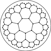
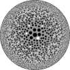
An infinite variety of regular polygonal lattices can be built on the Poincaré disk. All the lattices satisfy the relation , where is the number of edges of each polygon, and is the number of polygons around each vertex Firdy . The heptagonal lattice of is considered in the present work. Figure 1 shows the heptagonal lattice represented as a Poincaré disk. Although polygons depicted in the figure appear to be distorted, all of them are exactly congruent with the metric given in Eq. (3). The size of the entire lattice is characterized by the number of concentric layers of heptagons, denoted by , which effectively serves as the linear dimension of the lattice.

For a given , the total number of sites N is expressed by
| (7) |
where and ; refer to Appendix for the derivation of Eq. (7). The inset of Fig. 2 shows the semi-logarithmic plot of with . The plot shows that increases exponentially for . In fact, we obtain
| (8) |
which implies the boundary contribution quantified by does not become zero, but remains finite within the limit . It is emphasized that non-vanishing property of as well as the exponential increase in with is a result of the constant negative curvature of the underlying geometry, and it is the reason behind the non-trivial critical behavior of embedded lattices, as proved in previous studies Shima ; Shima2 .
III Numerical method
The current study aims at exploring the ordering mechanism of the heptagonal Ising model with ferromagnetic interaction. The Hamiltonian of the heptagonal Ising model is given by
| (9) |
where denotes a pair of nearest-neighbor sites on a lattice with free boundary conditions. The coupling strength is a constant, considering the fact that all the Ising spins are equally-spaced on the Poincaré disk. Throughout this paper, and are used as the units of temperature and energy, respectively. We have employed Monte Carlo simulations to calculate the order parameter and the two-point correlation function with . Here, represents the location of the th spin on the Poincaré disk, and the distance is a measure of the number of bonds along the shortest path between the th and th sites. Configuration space sampling has been carried out by using a cluster-flip algorithm Wolff , and averages have been calculated by considering samples.
IV Results and discussion
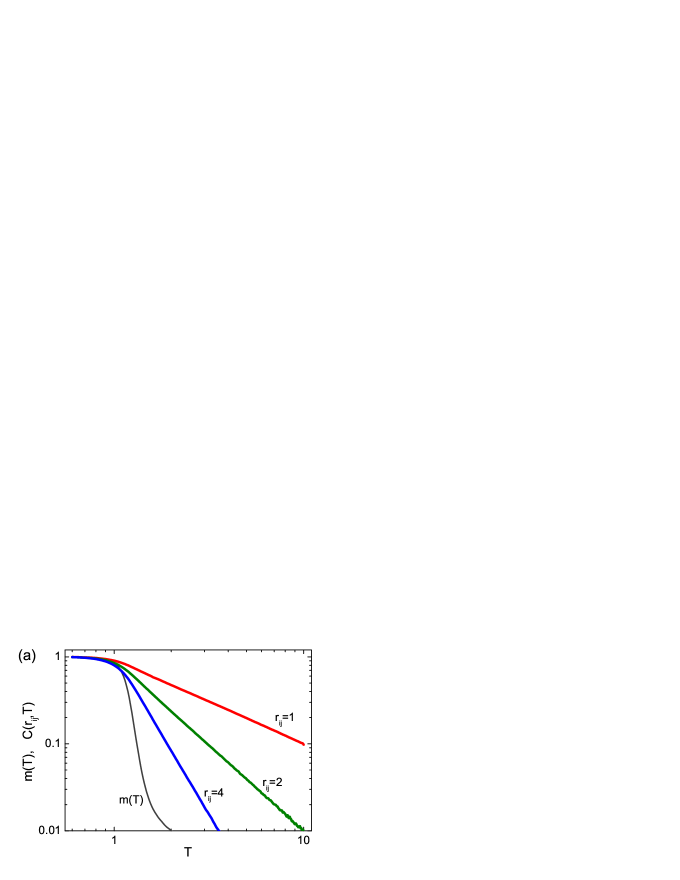
Figure 3 shows the temperature dependence of for different ’s. We have set (i.e., ) in all calculations. We found that for , shows power-law decay with and thus survive at Shima though is almost zero there. These survival of indicates that small-sized ferromagnetic domains remain active even at high temperatures, although they do not contribute to because of the change in sign between positive () and negative () domains. To explore the variety of domain sizes and examine boundary effects on size variations, we evaluate the correlation function, which is denoted by , of two spins that lie in the th layer. Figure 3(b) shows the -dependence of for , in which is varied from to (data for are omitted since they are indistinguishable from data for ). Interestingly, the data of for each value collapses onto a single curve at . This collapse implies that the domains that continue to exist at are of the same size and are uniformly scattered over the entire lattice, regardless of their distance from the outmost boundary.
It is emphasized that the persistence of domains at such high temperatures is supplementary to previous findings Auriac ; Shima related to low-temperature behaviors of an identical system. It was found that at , the central region of the lattice (far from the outmost boundary) exhibits an ordered phase that is a consequence of a mean-field transition Shima , while the outer region (close to the boundary) exhibits a stabilized Griffiths phase that is free from extrinsic disorder Auriac . Note that the former result indicates the presence of a paramagnetic phase in the central region at , where Ising spins are randomly oriented due to large thermal fluctuations. Hence, one would expect the formation of ferromagnetic domains to be hindered at ; however, contrary to the expectation, the formation is observed in the current simulations. This apparent contradiction is attributed to the finite-size effect. For a moderagely large , the strong boundary-spin contributions penetrate to the center of the lattice, as a result of which small-sized domains arise not only near the boundary but also in the central region. We conjecture that the domain in the central region disappears if a sufficiently large value of is considered: however, huge computational costs are involved when the value of is large enough.
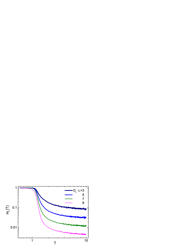
To gain a better insight into the above issue, we evaluate the quantity , where is a circular region enclosed by the th layer. Figure 4 shows the -dependence of for different values of . It is found that above , for is finite whereas becomes almost zero. This indicates an incomplete cancellation between the positive and negative domains in the region due to its small size. We emphasize that should become zero if is in the paramagnetic phase with no finite-sized domains. Therefore, the finiteness of at is another piece of evidence that supports the persistence of small-sized domains. We have also confirmed that finite at high tends to disappear with an increase in , since boundary-spin contributions are prevented from penetrating to the center of the lattice.
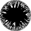
Figure 5 illustrates the ordering process of our moderately large Ising lattice with a decrease in the temperature. At , small-sized ferromagnetic domains (indicated by open and solid circles) are randomly embedded in the paramagnetic phase which is shown in gray. These domains are distributed homogeneously across the lattice, but give rise to finite for small values of due to the incomplete cancellation between the positive and negative domains. Subsequently, a decrease in results in the growth of domains within the inner region. Eventually, the ferromagnetic phase is formed through the mean-field phase transition. Nevertheless, near the outmost boundary, small domains remain active and fluctuate on a large time scale, as observed in Ref. Auriac .
V Conclusion
In the present work, we have considered the ordering mechanism of the Ising lattice model assigned to a negatively curved surface. We have found that small-sized domains survive at temperatures much higher than , at which the inner bulk region of the lattice goes through mean-field phase transition. The existence of small domains is attributed to the non-zero boundary-spin contribution that is unique to negatively curved surfaces. Our results are consistent with those of previous studies: the Griffiths phase is present near the outmost boundary of the lattice, while the inner core region undergoes the mean-field phase transition. This consistency sheds light on the nature of phase ordering in a wide variety of statistical lattice models assigned to negatively curved surfaces, most of which need to be further studied.

Acknowledgements
The authors are grateful to K. Yakubo, T. Hasegawa and T. Nogawa for fruitful discussions. Y.S is thankful for the financial support from JSPS Research Fellowships for Young Scientists. H.S acknowledges the support from the Executive Office for Research Strategy in Hokkaido University. This work was supported in part by Grant-in-Aid for Scientific Research from Japan Ministry of Education, Science, Sport and Culture. Numerical calculations were performed in part by facility at the Supercomputer Center, ISSP, University of Tokyo.
Appendix A Proof of the formula (5)
This Appendix is devoted to the derivation of Eq. (7) — the explicit form of as a function of . We classify all the congruent heptagons in the lattice into two groups: (i) heptagons having a common edge with the adjacent heptagon lying in the inner concentric layer (referred to as “”-heptagons) and (ii) those having two common edges with the adjacent one heptagon in the inner layer (referred to as “”-heptagons). Figure 6(a) illustrates our classification, in which either of the symbols or is assigned to all heptagons except for the central one.
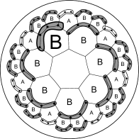
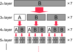
We see in Fig. 6 that the second innermost layer consists of seven ’s, the third innermost layer consists of 14 ’s and seven ’s, and so on. We identify the four sites within a hatched region as those attached to the -heptagon; in a similar way, the three sites enclosed by a curve are identified as those attached to the -heptagon. Then, we can say that the four sites of a -heptagon located at “engenders” one -heptagon and -heptagons at . Similarly, it follows that an -heptagon at generates a pair containing an -heptagon and a -heptagon at (although it is not shown in Fig. 6(a)). This proliferation process is summarized by the diagram in Fig. 6(a); each (or ) block symbolizes an ensemble of three (or four) sites, and a block in the th layer creates several blocks in the layer. The diagram illustrates a method to count the total number of sites contained in a given th layer.
We now have all the ingredients to derive the formula. Let us denote the number of - (or -) heptagons in the th layer by (or ) and set . It follows from the diagram that for any ,
| (10) |
We eliminate from Eq. (10) to obtain whose solutions under the conditions and are given by
| (11) |
where . Hence, we have for ,
| (12) |
where . As a result, the desired formula – Eq. (7) – for can be obtained.
References
- (1) L. Onsager, Phys. Rev. 65 (1944) 117.
- (2) B. Kaufman, Phys. Rev. 76 (1949) 1232.
- (3) M. E. Fisher, Rev. Mod. Phys. 70 (1998) 653.
- (4) R. Rietman, B. Nienhuis and J. Oitmaa, J. Phys. A: Math. Gen. 25 (1992) 6577.
- (5) O. Diego, J. Gonzalez and J. Salas, J. Phys. A: Math. Gen. 27 (1994) 2965.
- (6) Ch. Hoelbling and C. B. Lang, Phys. Rev. B 54 (1996) 3434.
- (7) J. González, Phys. Rev. E 61 (2000) 3384.
- (8) M. Weigel and W. Janke, Euro. Phys. Lett. 51 (2000) 578.
- (9) J. C. A. d’Auriac, R. Mélin, P. Chandra and B. Douçot, J. Phys. A: Math. Gen. 34 (2001) 675.
- (10) Y. Deng and H. W. J. Blöte, Phys. Rev. E 67 (2003) 036107.
- (11) R. Costa-Santos, Phys. Rev. B 68 (2003) 224423.
- (12) B. Doyon and P. Fonseca, J. Stat. Mech. (2004) 07002.
- (13) V. A. Kazakov, Phys. Lett. A 119 (1986) 140.
- (14) P. Di Francesco, P. Ginsparg and J. Zinn-Justin, Phys. Rep. 254 (1995) 1.
- (15) C. Holm and W. Janke, Phys. Lett. B 375 (1996) 69.
- (16) H. Yoshikawa, K. Hayashida, Y. Kozuka, A. Horiguchi and K. Agawa, Appl. Phys. Lett. 85 (2004) 5287.
- (17) G. B. Ji, H. L. Su, S. L. Tang, Y. W. Du, and B. L. Xu, Chem. Lett. 34 (2005) 86.
- (18) F. Liang, L. Guo, Q. P. Zhong, X. G. Wen, C. P. Chen, N. N. Zhang, and W. G. Chu, Appl. Phys. Lett. 89 (2006) 103105.
- (19) A. K. Srivastava, S. Madhavi, T. J. White, J. Mater. Res. 22 (2007) 1250.
- (20) L. Guo, F. Liang, N. Wang, D. Kong, S. Wang, L. He, C. Chen, X. Meng, and Z. Wu, Chem. Mater. 20 (2008) 5163.
- (21) A. Cabot, A. P. Alivisatos, V. F. Puntes, L. Balcells, Ó. Iglesias, and A. Labarta, Phys. Rev. B 79 (2009) 094419.
- (22) H. Shima and Y. Sakaniwa, J. Phys. A: Math. Gen. 39 (2006) 4921.
- (23) H. Shima and Y. Sakaniwa, J. Stat. Mech. (2006) 08017.
- (24) K. Ueda, R. Krcmar, A. Gendiar and T. Nishino, J. Phys. Soc. Jpn. 76 (2007) 084004.
- (25) H. S. M. Coxeter Introduction to Geometry (Wiley, New York) (1969)
- (26) P. A. Firdy and C.F. Gardiner Surface Topology (Ellis Horwood, London) (1991)
- (27) G. S. Milagre and W. A. Moura-Melo, Phys. Lett. A 368 (2007) 155.
- (28) I. Hasegawa, Y. Sakaniwa and H. Shima, Surf. Sci. 601 (2007) 5232.
- (29) Y. Sakaniwa, I. Hasegawa and H. Shima, J. Magn. Magn. Mater. 310 (2007) 1401.
- (30) I. Hasegawa, Y. Sakaniwa and H. Shima, J. Magn. Magn. Mater. 310 (2007) 1407.
- (31) S. K. Baek, P. Minnhagen and B. J. Kim, EPL 79 (2007) 26002.
- (32) L. R. A. Belo, N. M. Oliveira-Neto, W. A. Moura-Melo, A. R. Pereira and E. Ercolessi, Phys. Lett. A 365 (2007) 463.
- (33) W. A. Moura-Melo, A. R. Pereira, L. A. S. Mól and A. S. T. Pires, Phys. Lett. A 360 (2007) 472.
- (34) R. Krcmar, T. Iharagi, A. Gendiar and T. Nishino, Phys. Rev. E 78 (2008) 061119.
- (35) A. Gendiar, R. Krcmar, K. Ueda and T. Nishino, Phys. Rev. E 77 (2008) 041123.
- (36) R. Krcmar, A. Gendiar, K. Ueda and T. Nishino, J. Phys. A: Math. Theor. 41 (2008) 125001.
- (37) V. L. Carvalho-Santos, A. R. Moura, W. A. Moura-Melo and A. R. Pereira, Phys. Rev. B 77 (2008) 134450.
- (38) S. K. Baek, S. D. Yi and B. J. Kim, Phys. Rev. E 77 (2008) 022104.
- (39) S. K. Baek, P. Minnhagen and B. J. Kim, Phys. Rev. E 79 (2009) 011124.
- (40) S. K. Baek, H. Shima, and B. J. Kim, Phys. Rev. E 79 (2009) 060106(R).
- (41) S. K. Baek, P. Minnhagen, H. Shima, and B. J. Kim, arXiv:0904.3838.
- (42) F. Sausset and G. Tarjus, J. Phys. A: Math. Theor. 40 (2007) 12873.
- (43) C. D. Modes and R. D. Kamien, Phys. Rev. Lett. 99 (2007) 235701.
- (44) C. D. Modes and R. D. Kamien, Phys. Rev. E 77 (2008) 041125.
- (45) F. Sausset and G. Tarjus, Phil. Mag. 88 (2008) 4025.
- (46) F. Sausset, G. Tarjus and P. Viot, Phys. Rev. Lett. 101 (2008) 155701.
- (47) M. L. de Haro, A. Santos, S. B. Yuse J. Chem. Phys. 129 (2008) 116101
- (48) F. Sausset, G. Tarjus and P. Viot, J. Stat. Mech. (2009) P04022.
- (49) B. Jancovici and G. Téllez, J. Stat. Phys. 91 (1998) 953.
- (50) G. Téllez and E. Trizac, J. Chem. Phys. 118 (2003) 3362.
- (51) R. Fantoni, B. Jancovici and G. Téllez, J. Stat. Phys. 112 (2003) 27.
- (52) B. Jancovici and G. Téllez, J. Stat. Phys. 116 (2004) 205.
- (53) H. Shima, H. Yoshioka, and J. Onoe, Phys. Rev. B 79 (2009) 201401.
- (54) S. Ono and H. Shima, Phys. Rev. B 79 (2009) 235407.
- (55) N. L. Balazs and A. Voros, Phys. Rep. 143 (1986) 109.
- (56) J. E. Avron, M. Klein, A. Pnueli and L. Sadun, Phys. Rev. Lett. 69 (1992) 128.
- (57) A. Oloumi and D. Teychenné, Phys. Rev. E 60 (1999) R6279.
- (58) L. Horwitz, Y. B. Zion, M. Lewkowicz, M. Schiffer, and J. Levitan, Phys. Rev. Lett. 98 (2007) 234301.
- (59) E. D’Hoker and D. H. Phong, Rev. Mod. Phys. 60 (1988) 917.
- (60) J. Levin, Phys. Rep. 365 (2002) 251.
- (61) B. McInnes, Nucl. Phys. B 709 (2005) 213.
- (62) T. Nogawa and T. Hasegawa, J. Phys. A: Math. Theor. 42 (2009) 145001.
- (63) U. Wolff, Phys. Rev. Lett. 62 (1989) 361.