A high-order Godunov scheme for global 3D MHD accretion disks simulations. I. The linear growth regime of the magneto-rotational instability

We employ the PLUTO code for computational astrophysics to assess and compare the validity of different numerical algorithms on simulations of the magneto-rotational instability in 3D accretion disks. In particular we stress on the importance of using a consistent upwind reconstruction of the electro-motive force (EMF) when using the constrained transport (CT) method to avoid the onset of numerical instabilities. We show that the electro-motive force (EMF) reconstruction in the classical constrained transport (CT) method for Godunov schemes drives a numerical instability. The well-studied linear growth of magneto-rotational instability (MRI) is used as a benchmark for an inter-code comparison of PLUTO and ZeusMP. We reproduce the analytical results for linear MRI growth in 3D global MHD simulations and present a robust and accurate Godunov code which can be used for 3D accretion disk simulations in curvilinear coordinate systems.

1 Introduction

Most classical work on the MRI has been conducted using local shearing sheet simulations (Brandenburg et al., 1995; Hawley et al., 1995; Sano et al., 2004). Nevertheless, recent development has shown that critical questions about turbulence in accretion disks can only be addressed in global simulations, e.g. the saturation level of turbulence, the global evolution and the role of the global field configuration. So far most existing codes which can handle global disk simulations are based on a Zeus like finite difference scheme (Hawley, 2000; Fromang & Nelson, 2006, 2009). Thus, it would be very beneficial to have an independent method to attack the open questions in Magneto-Hydrodynamic disk simulations. The recently introduced MHD Godunov code PLUTO (Mignone et al., 2007) brought new insight into the field of jet propagation and for instance MHD simulations in the solar system, e.g. the space weather prediction. The latter example has the benefit that the predictions obtained with the numerical method can be tested against observation. A number of investigators have recognized the importance of using conservative Godunov-type upwind schemes rather than non-conservative finite difference algorithms which do not make use of the characteristic of the associated Riemann Problem. Clearly accretion disk calculations using conservative schemes are of great interest. As we want to apply our simulations to study the physical conditions for the planet formation process in circumstellar disks, we need not only the dynamical evolution of the disk, but also the detailed thermal and chemical conditions of the disk gas. None of the global disk simulations so far have been performed with tracing the temperature changes in the gaseous disk. The first result in this direction is comparing MRI linear growth rates including radiation transport which was achieved in local-box simulations (Flaig et al., 2009). It is widely accepted that the magneto-rotational instability (MRI) drives the turbulence in proto-planetary disks, leading to gas accretion onto the star as well as radial and vertical mixing. The efficiency of MRI-driven turbulence depends on the ionization degree of the gas. To determine the latter, thermal evolution including heat input from magnetic field dissipation has to be taken into account. Therefore we need an accurate conservative numerical scheme for treating such MHD processes as magnetic diffusion and reconnection in the presence of the small-scale turbulence. One of the most important challenges is an accurate and effective way to control and monitor the constraint of the divergence-free magnetic field. In the last years, several approaches on the numerical treatment of ${\rm div}(\mbox{\boldmath$B$})$ have been proposed. Two main classes for Godunov schemes have been established over the years. First, Powell’s ”Eight Waves” method uses the modified Euler equations with specific source terms and allows for magnetic monopoles treated as the $8^{\rm{th}}$ wave (Powell 1994). This idea is similar to the elliptical cleaning method (Dedner et al., 2002) which damps numerical monopoles. The second class is the Constrained Transport method, initially used as MocCT in ZEUS and then adapted to Godunov schemes (Balsara & Spicer, 1999). Here, the magnetic field components are always reprojected on the staggered grid and ${\rm div}(\mbox{\boldmath$B$})=0$ is kept within machine accuracy. The classical CT method for Godunov schemes (Balsara & Spicer, 1999) uses an arithmetic averaging of the electro-motive forces (EMF). This average proves to be not consistent with the plane parallel propagation in upwind schemes (Londrillo & Del Zanna, 2000). (Londrillo & del Zanna, 2004) have proposed a new way, named upwind constrained transport (UCT), of combining CT and a consistent upwind EMF reconstruction. Gardiner & Stone (2005) also developed a consistent method for the CT implementation in the ATHENA code. The PLUTO code offers a choice of the methods described above. The PLUTO code (Mignone et al., 2007) is a conservative multi-dimensional and multi-geometry code, with applications for Newtonian, relativistic, MHD and relativistic MHD fluids. The possibility of switching between several numerical modules in PLUTO allows us to perform a broad variety of test problems and choose the module with the best convergence and stability. E.g. the code offers the possibility of using Riemann solvers of ROE, HLLD, HLLC, HLL and Lax-Friedrich Rusanov. In this paper we investigate the applicability of the MHD methods for 3D curvilinear global simulations of the turbulent disk. To have comparable and reliable results, simulations with the ZEUS code are included in this paper, representing the group of the finite difference codes. ZeusMP version 1b has been used successfully for 3D MHD global simulations of astrophysical disks. ZeusMP (Stone & Norman, 1992; Hayes et al., 2006) has a classical staggered discretization of magnetic and electric vector fields (MoC CT). An identical model is set up in the actual ZeusMP code as well as the PLUTO 3. We examine the performance of the different numerical schemes by comparing the growth of the MRI with the expectations from linear analysis. The PLUTO code has successfully reproduced a series of standard MHD tests, including the rotating shock-tube, the fast rotor and the blast wave solution (Mignone et al., 2007). In addition, a magnetized accretion torus in 2.5 dimensions is demonstrated.
We are testing the PLUTO code specifically for the linear MRI. Our 3D disk setup allows to reproduce exactly the conditions for MRI typical for accretion disk studies. At the same time, unphysical results can easily be discovered by analytical linear MRI analysis. In section 2 we describe the differences in the numerical schemes of ZEUS and PLUTO. Section 3 presents our disk model used for linear MRI simulation and the measurement method. In Section 4 we show the results of the inter-code comparison. A convergence check for the chosen code configuration is investigated in section 5. Conclusion and outlook are given in section 6.

2 Numerics

2.1 MHD Equations

The equations of ideal magnetohydrodynamics written for Godunov schemes in conservative form are:

$$\frac{\partial\rho\mbox{\boldmath$u$}}{\partial t}+\nabla\cdot(\rho\mbox{\boldmath$u$}\mbox{\boldmath$u$}-\mbox{\boldmath$B$}\mbox{\boldmath$B$})=-\nabla P^{*}+\rho\nabla\Psi,$$ (1)

$$\frac{\partial\rho}{\partial t}+\nabla\cdot(\rho\mbox{\boldmath$u$})=0,$$ (2)

$$\frac{\partial\mbox{\boldmath$B$}}{\partial t}+\nabla\cdot(\mbox{\boldmath$u$}\mbox{\boldmath$B$}-\mbox{\boldmath$B$}\mbox{\boldmath$u$})=0,$$ (3)

and

$$\frac{\partial E}{\partial t}+\nabla\cdot((E+P^{*})\mbox{\boldmath$u$}-\mbox{\boldmath$B$}(\mbox{\boldmath$B$}\mbox{\boldmath$u$}))=\rho\mbox{\boldmath$u$}\nabla\Psi$$ (4)

where $\rho$ is the gas density, $\rho\mbox{\boldmath$u$}$ is the momentum density, $B$ is the magnetic field, and $E$ is the total energy density. The total pressure is a sum of magnetic and gas pressure, $P^{*}=P+(\mbox{\boldmath$B$}\cdot\mbox{\boldmath$B$})/2$. Total energy density is connected to internal energy $\epsilon$ as $E=\epsilon+\rho u^{2}/2+B^{2}/2$. Gravitational potential $\Psi=1/R$ is chosen in the normalized form to describe the sheared azimuthal flow of the gas, reproducing the Kepler rotation. We use cylindric coordinates in our models with the notation: $(R,\phi,Z)$. The equations are solved using uniform grids. In our runs we take an adiabatic approximation for the Equation of State, $P=(\gamma-1)\epsilon$, with $\gamma=5/3$.
Treatment in ZEUS: The equations (1-4) are solved by ZeusMP in a non-conservative way, i.e. the momentum conservation will be treated in the following way,

$$\rho\frac{{\rm d}\mbox{\boldmath$u$}}{{\rm d}t}=-\nabla P+\rho\nabla\Psi+\frac{1}{4\pi}[\nabla\times{}\mbox{\boldmath$B$}]\times{}\mbox{\boldmath$B$}.$$ (5)

As the vector components of velocity and magnetic fields are stored at the grid interfaces, fluxes can be calculate directly in ZEUS. Density and pressure are stored at the cell center and the vector values are at the interfaces. The scheme is second order in space and time. For time integration, ZEUS uses a Hancock scheme. Contrary to Zeus-type finite difference schemes, a Godunov type scheme, such as represented by the PLUTO code, follows a conservative model. Therefore the temperature can be exactly calculated from the total energy conservation. In general all quantities are stored at the cell center and an 2nd order Runge-Kutta (RK) iterator is employed. Prior to flux calculation, variables are reconstructed at the grid interface, which implies interpolation with a limited slope. The resulting two different states at the interfaces allow to solve the Riemann problem, which is the main feature of a Godunov code. CFL value is 0.25.

2.2 Magnetic fields in Godunov schemes

In case of MHD, cell-centered Godunov schemes have in general problems with occurring numerical magnetic monopoles (Balsara & Spicer, 1999). Powell’s ”8 wave” method includes this numerical magnetic monopoles as source terms. In the constrained transport (CT) MHD method, the magnetic fields are located at the interfaces. Usually, this method allows to handle the magnetic monopoles at machine accuracy. After updating the staggered magnetic field, the cell centered variables will be interpolated from the new interface values. The mainly used configuration in curvilinear coordinates systems consists of the second order upwind scheme with piece-wise linear reconstruction and RK 2 for time evolution. In our inter-code comparison we test Powell’s ”8 Waves” method, the CT scheme and the different MHD Riemann solvers of Roe (Cargo & Gallice, 1997), HLLD (Miyoshi & Kusano, 2005), HLL and Lax-Friedrich Rusanov. We must note that for the most frequently used configurations the ZEUS code has a speed up of factor 4. This factor appears because of the additional time step in the Runge Kutta time integration and the solving of the Riemann problem.

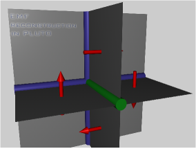
Figure 1: The reconstruction of the EMF (green axis) from four Godunov fluxes (red arrows) in case of arithmetic average of fluxes (ACT)

2.3 CT EMF reconstruction

The solenoidality of magnetic fields is difficult to represent correctly in Godunov schemes. The simple arithmetic average to reconstruct the EMF is presented in Fig. 1 and follows the Eq.(7)-Eq.(9) in Balsara & Spicer (1999). We share the opinion presented in Londrillo & Del Zanna (2000); Londrillo & del Zanna (2004), that such a simple hybrid method as ACT in Godunov scheme is not solving the monopole problem. The arithmetical CT algorithm is not consistent with the integration algorithm for plane-parallel, grid-aligned flows, as in our case with the dominating Kepler rotation. In PLUTO, the upwind CT scheme (UCT) follows Gardiner & Stone (2005) and is based on the work of Londrillo & Del Zanna (2000); Londrillo & del Zanna (2004). The main difference with respect to ACT is to construct the EMF update in such away that it is recovering the proper directional biasing (Gardiner & Stone, 2005). The first method is here called UCT.

$$\hat{\varepsilon}_{z,i+1/2,j+1/2}=\frac{1}{2}(\varepsilon_{z,i+1/2,j}+\varepsilon_{z,i+1/2,j+1}+\varepsilon_{z,i,j+1/2}+\varepsilon_{z,i+1,j+1/2})$$

$$-\frac{1}{4}(\varepsilon_{z,i,j}+\varepsilon_{z,i,j+1}+\varepsilon_{z,i+1,j}+\varepsilon_{z,i+1,j+1})$$

The term $\varepsilon_{z,i+1/2,j+1/2}$ is taken from the Godunov fluxes as illustrated in Fig. 1. $\varepsilon_{z,i,j}$ are the finite volume electric fields calculated from the cell center values. In addition to this method, we also test the EMF corner-integration, here called $\rm UCT_{CONTACT}$:

$$\epsilon_{z,i+1/2,j+1/2}=\frac{1}{4}(\epsilon_{z,i+1/2,j}+\epsilon_{z,i+1/2,j+1}+\epsilon_{z,i,j+1/2}+\epsilon_{z,i+1,j+1/2})$$

$$+\frac{\delta y}{8}((\frac{\partial\epsilon_{z}}{\partial y})_{i+1/2,j+1/4}-(\frac{\partial\epsilon_{z}}{\partial y})_{i+1/2,j+3/4})$$

$$+\frac{\delta x}{8}((\frac{\partial\epsilon_{z}}{\partial x})_{i+1/4,j+1/2}-(\frac{\partial\epsilon_{z}}{\partial x})_{i+3/4,j+1/2})$$

with

$$(\frac{\partial\epsilon_{z}}{\partial x})_{i+1/4,j}=\frac{2}{\delta x}(\epsilon_{z,i+1/2,j}-\epsilon_{z,i,j})$$

and

$$\left(\frac{\partial\epsilon_{z}}{\partial y}\right)_{i+1/2,j+1/4}=\left\{\begin{array}[]{ll}(\partial\epsilon_{z}/\partial y)_{i,j+1/4}&{\rm for}\ v_{x,i+1/2,j}>0,\\ (\partial\epsilon_{z}/\partial y)_{i+1,j+1/4}&{\rm for}\ v_{x,i+1/2,j}<0,\\ \frac{1}{2}((\partial\epsilon_{z}/\partial y)_{i,j+1/4}\\ +(\partial\epsilon_{z}/\partial y)_{i+1,j+1/4}),&\rm{otherwise}.\\ \end{array}\right)$$

The latter shows in general the same MRI evolution and therefor we concentrate on testing of UCT.

3 Linear MRI in global disk

The magneto-rotational instability (MRI) (Balbus & Hawley, 1991; Hawley & Balbus, 1991; Balbus & Hawley, 1998) is believed to occur in astrophysical disks. The analytical description of its linear stage has been discovered by Balbus & Hawley (1991).Local shearing box simulations have confirmed the analytical expectation of the linear MRI growth (Brandenburg et al., 1995; Hawley et al., 1995). Global simulations and also nonlinear evolution of the MRI was presented in Hawley & Balbus (1991). Our simplified setup here is representative for a global proto-planetary disk and made for a modest radial domain.

3.1 Global setup

Our disk model is not representing the whole 3D accretion disk, but a part which is large enough to fulfill global properties. The gas is rotating differentially with the Keplerian shear, $u_{\phi}^{2}=\frac{1}{R}$. There is no vertical stratification in both rotation and gas density. Initial temperature and density are constant in the entire disk patch, $\rho=\rho_{0}$, $T=T_{0}$, $c_{0}=0.1$. Therefore the orbital speed at the inner boundary in units of the sound speed is 10. The domain extends pi/3 radians in the azimuthal direction, $\rm{Z}=\pm 0.5$ and from 1 to 4 units in the radial direction. An annulus of uniform vertical magnetic field is placed at radii between 2 and 3 units, avoiding the radial boundaries so that any effects of the boundary conditions are reduced. The resolution is $[R,\phi,Z]=[128,64,64]$. For both codes we use identical random generated velocity perturbations ($10^{-4}u_{\rm Kep}$) for radial and vertical velocities as the initial seed for the turbulence. Boundary conditions are periodic for the vertical and azimuthal direction, and zero gradient for the radial one. Using the analytical prediction for the critical MRI wavelength, we choose the uniform vertical magnetic field strength in order to obtain the number of fastest-growing wavelengths fitting in the domain heigh, $B_{z}=0.05513/n$ where $n=1,2,...8$ (after equation 2.32 in Balbus & Hawley (1991)). The critical wavelength and the growth rate can be directly measured from our simulations and compared with the analytical prediction.

3.2 Limits of the MRI growth rate

Before using the growth rate as numerical benchmark, the physical processes limiting the growth rate in the linear MRI have to be considered. When magneto-rotational instability sets in, the magnetic fields are amplified with $B=B_{0}\exp({\gamma t})$ until they reach the saturation. Here we use a standard notation where $\gamma$ is the MRI growth rate. As it is mentioned in Hawley & Balbus (1991), the absolute limit of the growth rate for ideal MHD is given in case of zero radial wave vectors $q_{r}=0$ with the normalized wave vector $q_{z}$,

$$q_{z}=k_{z}\sqrt{16/15}\nu_{A}/\Omega.$$ (6)

with the Alvén speed $\nu_{A}=B/\sqrt{4\pi\rho}$. Then, the critical mode $q_{z}=0.97$ grows with $\gamma=0.75\Omega$, visible in Fig. 2. Like in Balbus & Hawley (1991b) we do not a priori know the radial wavenumber in our simulations. In Fig. 2 we plotted the growth rate for the amplitude of different vertical modes. The simulation is made for $B_{z}=0.05513/4$ with HLLD solver for resolution 128x64x64 (see also Table 2, $\rm{HLLD}_{\rm{LIN}}$). We have obtained the MRI growth rates which are comparable with Hawley & Balbus (1991),(Fig. 8). The addition limiters of the MRI growth rate are viscous and resistive dissipation (Pessah & Chan, 2008). We interpret the differences between the results, such as number of resolved MRI modes and the growth rate, as the effect of numerical dissipation which is individual for each solver.

Figure 2: Analytical growth rate is plotted for different $q_{r}$ (solid to dash-doted lines). The triangles present the measured MRI growth rates from our simulation with initial axisymmetric white noise disturbance from Model $\rm{HLLD}_{LIN}$ 128x64x64 with n=4. The values are measured for each radii and averaged. The results are similar to those in Hawley & Balbus (1991),(Fig. 8)

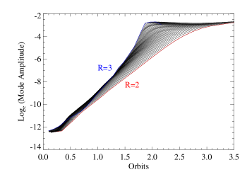
Figure 3: Maximal amplitude growth of the critical MRI mode is plotted for the 42 radial slices between radii $R=2$ and $R=3$ (solid lines). The setup is constructed to excite the mode with $\lambda_{\rm crit}=H$ ($n=1$). For the radii in the middle of MRI-active domain, the MRI growth rate reaches the value about $\gamma=0.75\Omega$. At the outer edge of the radial domain, the growth rate becomes higher than $0.75\Omega$. We suggest that the MRI modes there are affected from the inner part where MRI already breaks into nonlinear evolution.

In case of MRI, the numerical dissipation is the reason why we need some minimal amount of the grid cells to resolve the fastest growing MRI mode. Hawley et al. (1995) claim to need at least 5 grid cells per fastest growing mode. Generally, it holds that the more grid cells we use per critical mode the less is the numerical dissipation. But beside increasing resolution, changing the Riemann solver or the reconstruction method also affects the dissipation. The piece-wise linear method to reconstruct the interface states for the Riemann solver drives in general to higher numerical dissipation because of the additional interpolation. In ZEUS the velocity and magnetic fields are already at the interface and the fluxes can be calculated directly. For the inter-code comparison we use the setup described in section 3.1 with a vertical magnetic field with $n=4$. Then the resolution in Z is 16 grid cells per fastest growing mode which is also enough for very diffuse solvers. For better discerning between the code configurations we include also a weaker vertical magnetic field with $n=8$.

3.3 Measurement method

To reach the ideal limit and to explain our measurement method we set up a model with 1 critical mode (64 Grid cells per mode) to reduce the numerical dissipation (Fig. 3). In addition we use here a critical mode initial disturbance to enforce the MRI fastest mode to grow faster then any other waves. Fig. 3 shows the amplitude of the critical mode $\lambda_{z}$ visible in the radial magnetic field $B_{r}(Z)$. For each radial slice we use the local orbital time $T_{r}=2\pi R^{1.5}$ and calculate the growth rate between 1 and 1.5 local orbits. Most radial slices plotted in Fig. 3 show a growth rate close to the analytical limit. The inner annuli reach non-linear amplitudes first, producing disturbances that propagate outward and affect the development of the slower-growing linear modes in annuli further from the star. As a result the annuli near R=3 grow faster than indicated by the linear analysis in all the calculations with sufficient spatial resolution.

4 Inter code comparison

4.1 Energy evolution

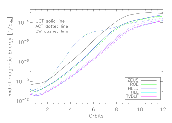
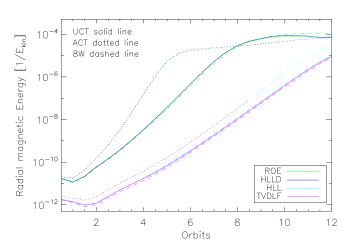
Figure 4: The total domain integrated radial magnetic energy plotted for n=4 (top) and n=8 (bottom) with upwind CT (solid line), Powell 8 wave (dashed line) and arithmetic CT (dotted line). The values are normalized over the initial orbital kinetic energy. After the initial disturbance, the growth of critical mode dominates and there is a linear MRI region visible between 2 and 8 inner orbits. For HLLD and Roe, the arithmetic CT shows a growth stronger then MRI until 5 inner orbits caused by a numerical instability. HLL and TVDLF have a much lower growth because both methods are viscous and do not resolve the critical mode for the adopted resolution.

Table 1 demonstrates the collection of models we made for inter-code comparison. The linear regime of MRI is visible in the total radial magnetic energy evolution, Fig. 4. The energy growth due to the excitation of the critical mode dominates after 2 inner orbits and the linear growth regime becomes visible. Fig. 4 shows the radial magnetic energy evolution for the 4 and 8 mode runs. In the 8 mode setups we can clearly distinguish 3 different classes of evolution. The Lax-Friedrich and HLL Riemann solver with all possible method of EMF reconstruction (ACT or CT with arithmetic EMF averaging, upwind CT and ”8 Wave”) have the slowest energy growth. The second group is built with the HLLD and Roe solvers with the upwind CT and the 8 wave method. Their results are most similar to ZEUS. The third group are the Roe and HLLD solver in combination with ACT (red colors in Table 1). The steep slope indicates a numerical problem. Table 1 presents the growth rate values for the different code configuration. The growth rates obtained from the model using the ACT scheme are higher than the analytical value.

Solver	$ACT_{n=4}$	$UCT_{n=4}$	$8W_{n=4}$	$ACT_{n=8}$	$UCT_{n=8}$	$8W_{n=8}$
ZEUS	$0.69\pm 0.03$	-	-	$0.69\pm 0.03$	-	-
HLLD	$0.68\pm 0.17$	$0.68\pm 0.03$	-	$0.86\pm 0.18$	$0.70\pm 0.03$	-
ROE	$0.70\pm 0.18$	$0.68\pm 0.03$	$0.68\pm 0.02$	$0.84\pm 0.18$	$0.70\pm 0.03$	$0.70\pm 0.04$
HLL	$0.64\pm 0.05$	$0.63\pm 0.05$	$0.61\pm 0.05$	$0.55\pm 0.09$	$0.51\pm 0.06$	$0.50\pm 0.06$
TVDLF	$0.64\pm 0.05$	$0.63\pm 0.05$	$0.63\pm 0.05$	$0.55\pm 0.09$	$0.51\pm 0.06$	$0.50\pm 0.06$

Table 1: MRI growth rates are measured for models with 4 and 8 MRI modes ($n=4,8$). Measurement of growth rates follows the description in section 3.3, $\gamma$ is averaged from the different radial shells. The growth rates higher than the analytical value are marked with red. The uncertainty numbers are measured from the radial variations in the growth rate visible in Fig. 7 or Fig. 9.

4.2 Arithmetic CT

In case of ACT and the high-resolution solver, the strong growth of magnetic energy overshoots the analytical expectation for MRI growth (Table 1 and Fig. 4). Here a numerical instability dominate s in the cases with the HLLD and Roe solvers. The fastest-growing mode has a vertical wavelength shorter than in the linear analysis. In Fig. 5 we plotted the growth rate for each radial slice, calculated from 1 to 1.5 local orbits. Roe and HLLD show the same unphysical high growth rate. On first inspection, the more diffusive HLL and TVDLF solvers seem not to be affected. However, at higher resolutions the numerical instability occurs there as well. The instability shows a ’checkerboard’ pattern (Fig. 5). The occurrence of such instabilities was already mentioned in Miyoshi & Kusano (2008). The Roe and HLLD solvers which include the Alfvén characteristic accurately evolve the disturbances independently of the resolution. The reason of the numerical instability lies in the inconsistent EMF reconstruction, as described in Londrillo & Del Zanna (2000). The correction methods are proposed in Londrillo & del Zanna (2004), Gardiner & Stone (2005) and Ziegler (2004). In short one can summarize, that the simple arithmetic average of 4 Godunov fluxes to reconstruct the EMF is not consistent with the upwind scheme. The error becomes visible in case of dominating flows along the azimuthal direction in 3D, presented in the Loop advection test from Gardiner & Stone (2005). It is interesting to note that the results of HLLD and Roe are very close. Also the values of HLL and TVDLF are exact the same in our tests. Resolving the Alfvén characteristic in MHD Riemann solver plays an important role for numerical dissipation.

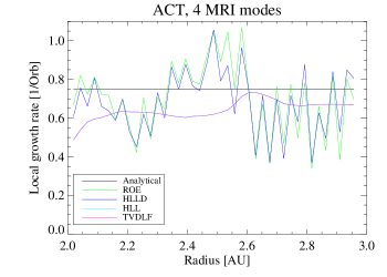
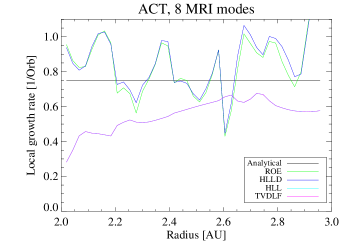
Figure 5: Local growth rate for n=4 (top) and n=8 (bottom) with arithmetic CT. For HLLD and Roe the local growth rate exceeds the analytical limit. The problem does not affect the HLL and TVDLF solver for the used resolution

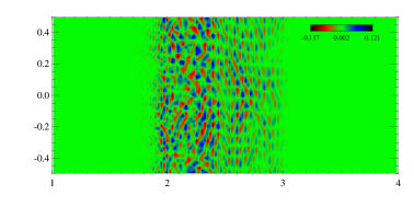
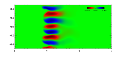
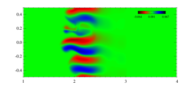
Figure 6: Contour plot of azimuthal magnetic field for arithmetic CT (top), UCT (middle) and ZEUS (bottom). In case of arithmetic CT, the numerical instability dominates MRI. In case for UCT and ZEUS the n=4 is visible. A change from blue to red means a change of magnetic field sign. The snap-shot of magnetic field is taken after 8 inner orbits.

4.3 Upwind CT vs 8 wave

With the Upwind CT EMF reconstruction the critical MRI mode dominates and ’checkerboard’ pattern disappears. Fig. 6 presents a contour plot of the azimuthal magnetic field. HLLD with upwind CT and ZEUS show 4 evolving modes. Fig. 7 shows the small difference between ”8 Waves” and upwind CT. The additional EMF corner-integration $\rm{UCT}_{CONTACT}$ does not change the result. The strongest effect on numerical dissipation has the change of Riemann solver.

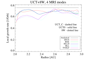
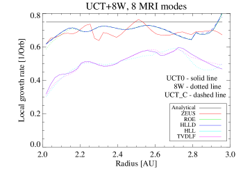
Figure 7: Local growth rate for n=4 (top) and n=8 (bottom) with upwind CT (solid line), $\rm{UCT}_{\rm{contact}}$ (dashed line) and Powell’s Eight Wave (dotted line). The high resolution MHD Riemann Solver HLLD and Roe show the same MRI evolution, producing same growth rate as ZEUS. HLL and TVDLF are more diffusive.

The reason is the number of wave characteristics which is used by each solver. HLL and TVDLF use the fast magneto-sonic wave characteristic as maximal signal velocity. HLLD includes additional the Alfvén wave characteristic and the contact discontinuity. The ROE solver includes all 7 MHD waves, as well as the slow magneto-sonic characteristic. ZEUS shows the MRI development same as HLLD and Roe.

4.4 4 to 8 MRI modes

In case of 4 modes, the resolution in the Z direction is sufficient for all Riemann solvers to resolve the critical mode. HLLD , Roe and ZEUS shows the highest growth rate followed by TVDLF and HLL. As already presented in Fig. 4. The models for 8 MRI critical modes are summarized in Table 1. Energy evolution is shown in Fig.4 (bottom). Growth rates are significantly reduced only for HLL and TVDLF solvers. ZEUS and the MHD Riemann solver ROE and HLLD resolve 7 modes, HLL and TVDLF only 4 modes. The resolution about 8 grid cells per critical mode is not enough to resolve the modes perfectly. Nevertheless, the additional Alfvén characteristic included in the HLLD solver drives to lower numerical diffusion. Fig. 8 shows a contour plot of radial magnetic field after 7 inner orbits for HLLD solver and ZEUS. The ZEUS code shows the MRI pattern very close to those of HLLD and Roe.

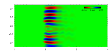
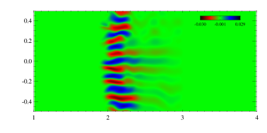
Figure 8: Contour plot of radial magnetic field in code units for the HLLD solver (top) and ZEUS (Bottom). After 7 inner orbits the inner radial part breaks into nonlinear regime. This affects also the growth rate at the outer part as we have already seen.

4.5 PPM vs PLM

The reconstruction of the states at the interfaces leads to the high dissipation in the Godunov schemes (see section 2). Therefore we test the fourth order piece-wise parabolic method (PPM) by Collela (1984) for the ROE,HLLD and for the diffusive TVDLF solver.

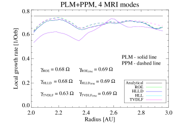
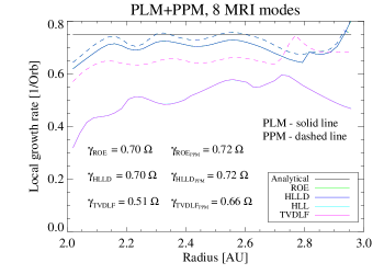
Figure 9: MRI growth rate for PPM (dashed) and PLM (solid). In the case of the Lax-Friedrich solver, the PPM interpolation leads to a lower numerical dissipation and growth rates nearer the analytic solution. Differences between HLLD and ROE solvers are negligible.

Fig. 9 shows the difference in local MRI growth rate for simulations made for interpolations with piece-wise linear method (PLM) and PPM. The results of MHD Riemann solver HLLD and ROE are not strongly affected, though there is a slightly lower numerical dissipation visible when PPM is used. But there is a strong effect of the interpolation method visible for the classical Lax-Friedrich and HLL solvers. In case of the 8 mode run, also the classical Riemann solver presents 7 modes and the values of ROE, HLLD and TVDLF converge. To verify this conclusion we investigate the resolution convergence, including only the HLLD and TVDLF solver with upwind CT and both reconstruction methods.

5 Convergence test

The models for the convergence tests are summarized in Table 2. We take here the n=4 model. We double the resolution up to 4 times for each dimension to check for the earliest convergence. In these runs we use an initial axisymmetric white noise for the radial and vertical velocity (www.random.org). This leads to slightly different growth rate values as in Table 1. Fig. 10 shows the results. The HLLD MHD Riemann solver in combination with piece-wise parabolic reconstruction shows the earliest convergence. Even with a resolution about 32 in Z and with the PPM reconstruction, we can resolve the critical mode and get the converged value of about $\gamma=0.70\Omega$ (Table 2). The resolution runs marked with a star do not resolve the fastest growing MRI mode. As expected, the Lax Friedrich solver shows the highest numerical dissipation. Here 8 grid cells per fastest growing mode are not enough. For the highest resolution of 512x256x256 we see in all cases a decreasing of the growth rate. We cannot say whether this behavior is connected with the presence of high radial wavenumber or a change in the numerical dissipation. All except the Zeus runs decline by less than the uncertainty.

Solver	32x16x16	64x32x32	128x64x64	256x128x128	512x256x256
$\rm{ZEUS}_{\rm{LIN}}$	0.58*$\pm$0.07	0.65$\pm$0.05	0.70$\pm$0.07	0.68$\pm$0.05	0.62$\pm$0.05
$\rm{HLLD}_{\rm{LIN}}$	0.53*$\pm$0.07	0.65$\pm$0.07	0.70$\pm$0.05	0.70$\pm$0.03	0.68$\pm$0.05
$\rm{HLLD}_{\rm{PPM}}$	0.60*$\pm$0.05	0.70 $\pm$0.06	0.71$\pm$0.05	0.71$\pm$0.04	0.67$\pm$0.04
$\rm{TVDLF}_{\rm{LIN}}$	0.33*$\pm$0.05	0.53*$\pm$0.09	0.65$\pm$0.05	0.70$\pm$0.04	0.67$\pm$0.04
$\rm{TVDLF}_{\rm{PPM}}$	0.50*$\pm$0.05	0.63*$\pm$0.08	0.72$\pm$0.06	0.70$\pm$0.03	0.67$\pm$0.04

Table 2: Growth rates for the resolution tests. The asterisks mark the runs which was not able to resolve n=4.

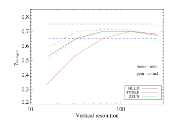
Figure 10: Growth rates exhibit a quick convergence to the $\gamma\sim 0.7$ with increasing resolution for all Godunov solvers, with the TVDLF solver performing notably worse. The dashed lines are marking the uncertainty of growth rate measurements. A decline is apparent at the highest resolution.

6 Conclusion

The inter-code comparison and the convergence test stress the importance of treating the Alfvén characteristics for MHD Riemann solver in MRI simulations. Observing the consequences implied by numerical dissipation, we obtain a robust and accurate Godunov scheme for 3D MHD simulation in curvilinear coordinate systems. The arithmetic average of the 4 Godunov fluxes (Balsara & Spicer, 1999) is not consistent with the upwind Godunov scheme (Londrillo & Del Zanna, 2000) and leads to numerical instability. Beside the loop advection test (Gardiner & Stone, 2008), the linear MRI evolution in global disks is a crucial test for a consistent MHD method. Our 3D MHD simulation with ACT show the unphysical behavior of a ’chessboard’ instability, mentioned for the HLLD solver in Miyoshi & Kusano (2008). The high-order MHD Riemann solvers HLLD and ROE, which contain the Alfvén characteristic, reproduce the ’chessboard’ pattern in the classical ACT scheme independent of resolution.

The upwind EMF reconstruction in combination with the accurate and robust HLLD MHD Riemann solver represents a good tool for future simulations of 3D MHD accretion disks. We reproduce the linear MRI analysis in the inter-code comparison. The Lax-Friedrich and HLL solvers demonstrate much higher numerical dissipation in comparison to the finite difference scheme ZEUS. The high-order MHD Riemann solver HLLD and ROE can compensate this dissipation by using more MHD characteristics. The Alfvén characteristic appears to play an important role for MRI. For the linear MRI evolution both HLLD and ROE show the same numerical dissipation as the finite difference scheme ZEUS. In addition, the HLLD solver shows nearly the exact evolution like ROE, even without resolving the slow magneto-sonic characteristic. In combination with the piece-wise parabolic method the HLLD solver has the earliest convergence compared to the Lax-Friedrich solver and ZEUS.

7 Outlook

The Prandtl numbers in global simulations for the high-order MHD Riemann solver and physical dissipation are very important for MRI turbulence in proto-planetary disks. Proper MHD tests shall be done, exploring the numerical dissipation of the PLUTO code. Fromang & Papaloizou (2007) measured the numerical Prandtl number for ZEUS, which is in the region from 2 to 8. Recent work by Simon et al. (2009) presented a Prandtl number about 2 for the Godunov type ATHENA code. Nevertheless, in the proto-planetary disks one can expect rather smaller Prandtl numbers, $\rm Pm<1$. The consequences of numerical $\rm Pm$ for MRI shall be explored.

Acknowledgments.

We thank Udo Ziegler for the very useful discussions about the upwind Constrained transport property. We also thank Neal Turner, Thomas Henning and Matthias Griessinger for the post process of this work. H. Klahr, N. Dzyurkevich and M. Flock have been supported in part by the Deutsche Forschungsgemeinschaft DFG through grant DFG Forschergruppe 759 ”The Formation of Planets: The Critical First Growth Phase”. Parallel computations have been performed on the PIA cluster of the Max-Planck Institute for Astronomy Heidelberg located at the computing center of the Max-Planck Society in Garching.

References

- Balbus & Hawley (1991) Balbus S.A., Hawley J.F., Jul. 1991, ApJ, 376, 214
- Balbus & Hawley (1998) Balbus S.A., Hawley J.F., Jan. 1998, Reviews of Modern Physics, 70, 1
- Balsara & Spicer (1999) Balsara D.S., Spicer D.S., Mar. 1999, Journal of Computational Physics, 149, 270
- Brandenburg et al. (1995) Brandenburg A., Nordlund A., Stein R.F., Torkelsson U., Jun. 1995, ApJ, 446, 741
- Cargo & Gallice (1997) Cargo P., Gallice G., Sep. 1997, Journal of Computational Physics, 136, 446
- Dedner et al. (2002) Dedner A., Kemm F., Kröner D., et al., Jan. 2002, Journal of Computational Physics, 175, 645
- Flaig et al. (2009) Flaig M., Kissmann R., Kley W., Mar. 2009, MNRAS, 282–+
- Fromang & Nelson (2006) Fromang S., Nelson R.P., Oct. 2006, A&A, 457, 343
- Fromang & Nelson (2009) Fromang S., Nelson R.P., Mar. 2009, A&A, 496, 597
- Fromang & Papaloizou (2007) Fromang S., Papaloizou J., Dec. 2007, A&A, 476, 1113
- Gardiner & Stone (2005) Gardiner T.A., Stone J.M., May 2005, Journal of Computational Physics, 205, 509
- Gardiner & Stone (2008) Gardiner T.A., Stone J.M., Apr. 2008, Journal of Computational Physics, 227, 4123
- Hawley (2000) Hawley J.F., Jan. 2000, ApJ, 528, 462
- Hawley & Balbus (1991) Hawley J.F., Balbus S.A., Jul. 1991, ApJ, 376, 223
- Hawley et al. (1995) Hawley J.F., Gammie C.F., Balbus S.A., Feb. 1995, ApJ, 440, 742
- Hayes et al. (2006) Hayes J.C., Norman M.L., Fiedler R.A., et al., Jul. 2006, ApJS, 165, 188
- Londrillo & Del Zanna (2000) Londrillo P., Del Zanna L., Feb. 2000, ApJ, 530, 508
- Londrillo & del Zanna (2004) Londrillo P., del Zanna L., Mar. 2004, Journal of Computational Physics, 195, 17
- Mignone et al. (2007) Mignone A., Bodo G., Massaglia S., et al., May 2007, ApJS, 170, 228
- Miyoshi & Kusano (2005) Miyoshi T., Kusano K., Sep. 2005, Journal of Computational Physics, 208, 315
- Miyoshi & Kusano (2008) Miyoshi T., Kusano K., Apr. 2008, In: Pogorelov N.V., Audit E., Zank G.P. (eds.) Numerical Modeling of Space Plasma Flows, vol. 385 of Astronomical Society of the Pacific Conference Series, 279–+
- Pessah & Chan (2008) Pessah M.E., Chan C.k., Sep. 2008, ApJ, 684, 498
- Powell (1994) Powell K.G., Mar. 1994, Approximate Riemann solver for magnetohydrodynamics (that works in more than one dimension), Tech. rep.
- Powell et al. (1999) Powell K.G., Roe P.L., Linde T.J., Gombosi T.I., de Zeeuw D.L., Sep. 1999, Journal of Computational Physics, 154, 284
- Sano et al. (2004) Sano T., Inutsuka S.i., Turner N.J., Stone J.M., Apr. 2004, ApJ, 605, 321
- Simon et al. (2009) Simon J.B., Hawley J.F., Beckwith K., Jan. 2009, ApJ, 690, 974
- Stone & Norman (1992) Stone J.M., Norman M.L., Jun. 1992, ApJS, 80, 753
- Ziegler (2004) Ziegler U., May 2004, Journal of Computational Physics, 196, 393