DESY 09-099 ISSN 0418-9833

June 2009

Chargino and Neutralino Separation with the ILD Experiment

T. Suehara¹, J. List²

1- International Center for Elementary Particle Physics

The University of Tokyo, Hongo 7-3-1, Bunkyo District

Tokyo 113-0033, Japan

2- Deutsches Elektronen Synchrotron DESY

Notkestr. 85

D-22607 Hamburg, Germany

One of the benchmark processes for the optimisation of the detector concepts proposed for the International Linear Collider is Chargino and Neutralino pair production in an mSugra scenario where $\tilde{\chi}^{\pm}_{1}$ and $\tilde{\chi}^{0}_{2}$ are mass degenerate and decay into $W^{\pm}\tilde{\chi}^{0}_{1}$ and $Z^{0}\tilde{\chi}^{0}_{1}$, respectively. In this case the separation of both processes in the fully hadronic decay mode is very sensitive to the jet energy resolution and thus to the particle flow performance. The mass resolutions and cross-section uncertainties achievable with the ILD detector concept are studied in full simulation at a center of mass energy of 500 GeV, an integrated luminosity of 500 fb^-1 and beam polarisations of $P(e^{+},e^{-})=(30\%,-80\%)$. For the $\tilde{\chi}^{\pm}_{1}$ and $\tilde{\chi}^{0}_{2}$ pair production cross-sections, statistical precisions of 0.84% and 2.75% are achieved, respectively. The masses of $\tilde{\chi}^{\pm}_{1}$, $\tilde{\chi}^{0}_{2}$ and $\tilde{\chi}^{0}_{1}$ can be determined with a statistical precision of 2.9 GeV, 1.7 GeV and 1.0 GeV, respectively.

Submitted to Eur. Phys. J. C

1 Introduction

In anticipation of the International Linear Collider (ILC), a proposed $e^{+}e^{-}$ collider with center-of-mass energies between 90 and 500 GeV, upgradable to 1 TeV, and polarised beams, several detector concepts are being discussed. In order to evaluate the performance of these concepts, benchmark processes have been chosen which are challenging for key aspects of the detector designs [1].

In order to test the jet energy resolution, a supersymmetric scenario which assumes non-universal soft SUSY-breaking contributions to the Higgs masses has been defined. In this scenario, the mass differences between the lightest SUSY particle (LSP) and the heavier gauginos become large, while at the same time the sleptons are so heavy that gaugino decays into sleptons are kinematically forbidden. The corresponding benchmark point has been defined in [1] as “Point 5” with the following SUSY parameters:

$$m_{0}=206~{}\mathrm{GeV,}\quad m_{1/2}=293~{}\mathrm{GeV,}\quad\tan{\beta}=10,\quad A=0,\quad\mu=375~{}\mathrm{GeV}$$ (1)

With a top quark mass of $M_{t}=178$ GeV, the following gaugino masses are obtained by Spheno [2]:

$$M_{\tilde{\chi}^{0}_{1}}=115.7~{}\mathrm{GeV,}\quad M_{\tilde{\chi}^{\pm}_{1}}=216.5~{}\mathrm{GeV,}\quad M_{\tilde{\chi}^{0}_{2}}=216.7~{}\mathrm{GeV,}\quad M_{\tilde{\chi}^{0}_{3}}=380~{}\mathrm{GeV}.$$ (2)

The lightest sleptons are even heavier than the gauginos, thus leading to branching fractions of 99.4% for the decay $\tilde{\chi}^{\pm}_{1}\rightarrow W^{\pm}\tilde{\chi}^{0}_{1}$ and 96.4% for $\tilde{\chi}^{0}_{2}\rightarrow Z^{0}\tilde{\chi}^{0}_{1}$:

$$M_{\tilde{\tau}_{1}}=230.8~{}\mathrm{GeV}\qquad M_{\tilde{e}_{R}}=237.4~{}\mathrm{GeV}$$ (3)

In order to benchmark the jet energy reconstruction, the fully hadronic decay mode of the gauge bosons is considered here. In this mode, Chargino and Neutralino events can only be separated via the mass of the vector bosons they decay into. The motivation of this study is not to evaluate the final precision which could be achieved at the ILC by combining several final states, or even by performing threshold scans, but to test the detector performance in the most challenging decay mode.

The analysis is performed at a center of mass energy of 500 GeV for an integrated luminosity of 500 fb^-1 with beam polarisations of $P(e^{+},e^{-})=(30\%,-80\%)$. It is based on a detailed simulation of the ILD detector based on GEANT4 [3], which is described briefly in the next section. Section 3 discusses the event reconstruction and selection procedure, including a pure Standard Model control selection. The results for the cross-section and mass measurement are presented in sections 4 and 5, respectively.

2 The ILD Detector Concept and its Simulation

The proposed ILD detector has been described in detail in the ILD Letter of Intent [4]. Its main characteristics comprise a time projection chamber as a main tracking device, which is complemented by silicon tracking and vertexing detectors, and highly granular electromagnetic and hadronic calorimeters as required for the particle flow approach [5]. Both, tracking system and calorimeters, are included in a solenoidal magnetic field with a strength of 3.5 T provided by a superconducting coil. The magnetic flux is returned in an iron yoke, which is instrumented for muon detection. Special calorimeters at low polar angles complement the hermeticity of the detector and provide luminosity measurement.

While previous studies were based on fast simulation programs which smear four-vectors with expected resolutions, we have used a full GEANT4 based simulation of all ILD compoments. Many details are included, in particular gaps in the sensitive regions and realistic estimates of dead material due to cables, mechanical support, cooling and so on.

With this detector simulation, the following performance has been achieved [4]: For tracks with a transverse momentum $p_{t}$ larger than 1 GeV, the tracking efficiency is 99.5% across almost the entire polar angle range of $|\cos{\theta}|<0.995$ covered by the tracking detectors, with a $p_{t}$ resolution of better than $\sigma_{1/p_{t}}=2\times 10^{-5}\oplus 1\times 10^{-3}/(p_{t}\sin{\theta})$. The calorimetric system has been designed to deliver a jet energy resolution of 3.0% to 3.7% over a large range of energies from 250 GeV down to 45 GeV for polar angles $\theta$ in the range $|\cos{\theta}|<0.9$. The luminosity is expected to be known to $10^{-3}$ from measurements of the Bhabha scattering cross-sections at small angles. The beam polarisations and the beam energies will be measured to $\delta P/P=0.25\%$ and $2\times 10^{-4}$, respectively by dedicated instrumentation in the beam delivery system.

The event sample used in this analysis has been generated using the matrix element generator Whizard [6]. It comprises all Standard Model processes plus all kinematically accessible SUSY processes in the chosen scenario. In total, about $12\times 10^{6}$ events have been generated and processed through the full simulation and reconstruction chain for this analysis.

3 Event Reconstruction and Selection

The reconstruction and also the first event selection steps are implemented in the MarlinReco framework [7]. The central part of the reconstruction for this analysis is the particle flow algorithm Pandora [5], which forms charged and neutral particle candidates - so-called “particle flow objects” or PFOs - from tracks and calorimeter clusters. The resulting list of PFOs for each event is forced into a 4–jet configuration using the Durham algorithm. The jet energy scale is raised by 1%, determined from dijet samples. No special treatment of b-quark jets is considered here.

As a final step of the reconstruction, a constrained kinematic fit [8], which requires the two dijet masses of the event to be equal, is performed on each event. All three possible jet pairings are tested. The resulting improvement in mass resolution is evaluated on Standard Model events, as described in section 3.2.

3.1 SUSY Selection

The major part of the Standard Model events is rejected by applying the following selection to all events in the SUSY and SM samples:

• In order to eliminate pure leptonic events, the total number of tracks in the event should be larger than $20$ and each jet has to contain at least two tracks.

• Since the two LSPs escape undetected, the visible energy of the event $E_{\mathrm{vis}}$ should be less than 300 GeV. In order to remove a substantial fraction of 2-photon events with very low visible energy, $E_{\mathrm{vis}}>100$ GeV is required as well.

• To ensure a proper jet reconstruction, each jet should have a reconstructed energy of at least 5 GeV and a polar angle $\theta$ fulfilling $|\cos(\theta_{\mathrm{jet}})|<0.99$.

• 2-jet events are rejected by requiring the distance parameter of the Durham jet algorithm for which the event flips from 4-jet to 3-jet configuration, $y_{34}$ to be larger than 0.001.

• Coplanar events (e.g. $W^{+}W^{-}$ with ISR/beamstrahlung photons) are removed by requiring $|\cos(\theta)|$ of the missing momentum  to be smaller than 0.99.

• No lepton candidate with an energy larger than 25 GeV is allowed in order to suppress semi-leptonic events.

The upper part of table 1 shows the reduction for these cuts. The selection efficiency of hadronic Chargino and Neutralino pair events is very high, 88.1% and 90.8%, respectively. Therefore, we will refer to this stage in the selection process as “high efficiency” selection. Although the SM background is significantly reduced already by these cuts, the contribution from 4-fermion events is still large, about 6 times the Chargino signal.

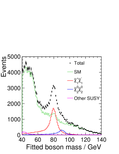
Figure 1: a) Reconstructed mass of the vector boson candidates after all selection cuts and kinematic fit for the jet pairing with the highest fit probability. b) Same distribution after some additional cuts to enhance the purity.

Figure 1a) shows the reconstructed boson mass distribution as obtained by the constrained kinematic fit after these selection cuts. A large fraction of the remaining Standard Model background features low invariant dijet masses, but nevertheless a sizable amount of background remains also in the signal region.

For the cross-section measurement, the sample is therefore cleaned further by four additional cuts:

• The number of particle flow objects (PFOs) in each jet should be $N_{\mathrm{PFO}}>3$ in order to reject $\tau$ jets more effectively.

• The direction of the missing momentum should fulfill $|\cos{\theta_{\mathrm{pmiss}}}|<0.8$: This cut is quite powerful to reject all kinds of SM backgrounds, which tend to peak in the forward region, while the signal follows a flat $\cos{\theta_{\mathrm{pmiss}}}$ distribution. Nevertheless, it reduces the signal efficiency substantially, which could be avoided for example by placing a more stringent cut on the missing mass instead (see next item). However, the missing mass distribution of the signal directly depends on the LSP mass, thus it should not be too finely tuned to specific mass values, since we want to measure the gaugino masses. The prediction of a flat $\cos{\theta_{\mathrm{pmiss}}}$ distribution depends only on the spin, and can thus be considered model-independent (within SUSY).

• The missing mass should be larger than 220 GeV to further reject 6-fermion events (semi-leptonic $t\bar{t}$). The value of this cut is chosen such that it is in a region with no SUSY contribution, i.e. where the data should agree with the SM expectation. Thus in a real experiment an adequate cut position could be found from the data. For this reason, no upper cut is placed on $M_{\mathrm{miss}}$, since other SUSY processes contribute there, and it would not be trivial to determine a suitable cut value from real data.

• The kinematic fit constraining the two dijet masses to be equal should converge for at least one jet pairing: This is necessary in order to use the fit result for further analysis. The efficiency and resolution of the fit can be cross-checked easily on real data, for instance with the control selection decribed in the previous section.

The obtained reduction due to these cuts is shown in the last four lines of table 1. The final distribution of the reconstructed boson mass, again obtained by the constrained kinematic fit, is displayed in figure 1b. It illustrates the achieved boson mass resolution and thus $W$ and $Z$ pair separation, however at significantly reduced efficiency. Fitting the total spectrum by a fourth order polynomial for the background plus the sum of two Breit-Wigner functions folded with a Gaussian for the $W$ and $Z$ contributions, the mass resolutions can be determined to 3.4 %.

Table 2 shows the final purity and efficiency of signal and major background processes. According to this table, $e^{+}e^{-}\rightarrow qqqq$ is the dominant process in the remaining background.

3.2 Standard Model Control Selection

Since the Chargino and Neutralino separation relies on reconstructing the masses of the $W$ and $Z$ bosons from their decay products, the dijet mass resolution is a crucial parameter in this analysis and has to be determined from Standard Model $W$ and $Z$ pair events. For this purpose, the “high efficiency” selection from above is applied to all simulated data, inverting only the cut on the visible energy to $E_{\mathrm{vis}}>300$ GeV. This yields an event sample which is vastly dominated by 4-fermion events, with a small contribution from 6-fermion events, but no SUSY events. The corresponding dijet mass spectrum is shown in figure 2.

The mass resolution has been determined for two cases:

• The jet pairing is chosen such that the difference between the two dijet masses in each event is minimized.

• A kinematic fit, which constrains the two dijet masses in each event to be equal, is performed for all three possible jet-boson associations. The jet pairing which yields the highest fit probability is chosen.

The resulting mass distributions are fitted with the sum of two Breit-Wigner functions convoluted with a Gaussian, fixing the $W$ and $Z$ widths as well as the $Z$ pole mass to their PDG values and having the same $\sigma$ for both Gaussians, plus a forth order polynomial for all non-resonant contributions.

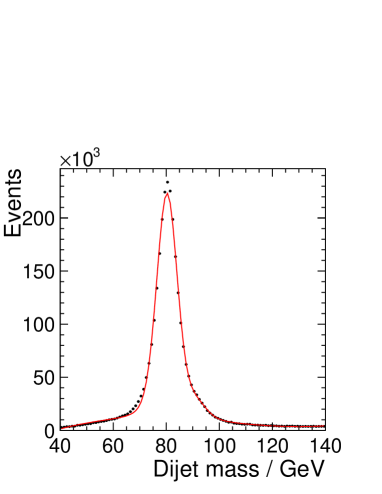
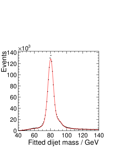
Figure 3: Dijet mass distributions a) without and b) with kinematic fit. Fitting the distributions with the sum of two Breit-Wigner functions folded with Gaussian plus a forth order polynomial for the non-resonant background yields dijet mass resolutions of 3.5 GeV (case a) and 3.0 GeV (case b).

Figure 3 shows the fitted spectra and the resulting fit parameters. In case a), without the kinematic fit, the dijet mass resolution is determined as $\sigma_{m}^{a}=3.5$ GeV, while it is reduced to $\sigma_{m}^{b}=3.0$ GeV when the kinematic fit is applied.

These mass resolutions are even better than in the SUSY case, since the kinematics of the events is more favourable here. While the SM gauge boson pairs are highly boosted and thus finding the correct jet pairing is relatively easy, the bosons in our SUSY scenario are produced nearly at rest, resulting in a higher combinatorical background and a slightly worse boson mass resolution. Nevertheless, a SM control selection will be crucial to demonstrate the level of detector understanding, since the actual SUSY measurement will rely on template distributions and selection efficiencies determined from simulations.

4 Cross-Section Measurement

The cross-sections of $e^{+}e^{-}\rightarrow\tilde{\chi}^{+}_{1}\tilde{\chi}^{-}_{1}$ and $e^{+}e^{-}\rightarrow\tilde{\chi}^{0}_{2}\tilde{\chi}^{0}_{2}$ can be measured by determining the amount of $W$ and $Z$ pair like events. For the hadronic events we are concerned with here, a 2-dimensional fit in the plane of the two dijet masses per event is performed to obtain the amount of $W$ and $Z$ pair candidates.

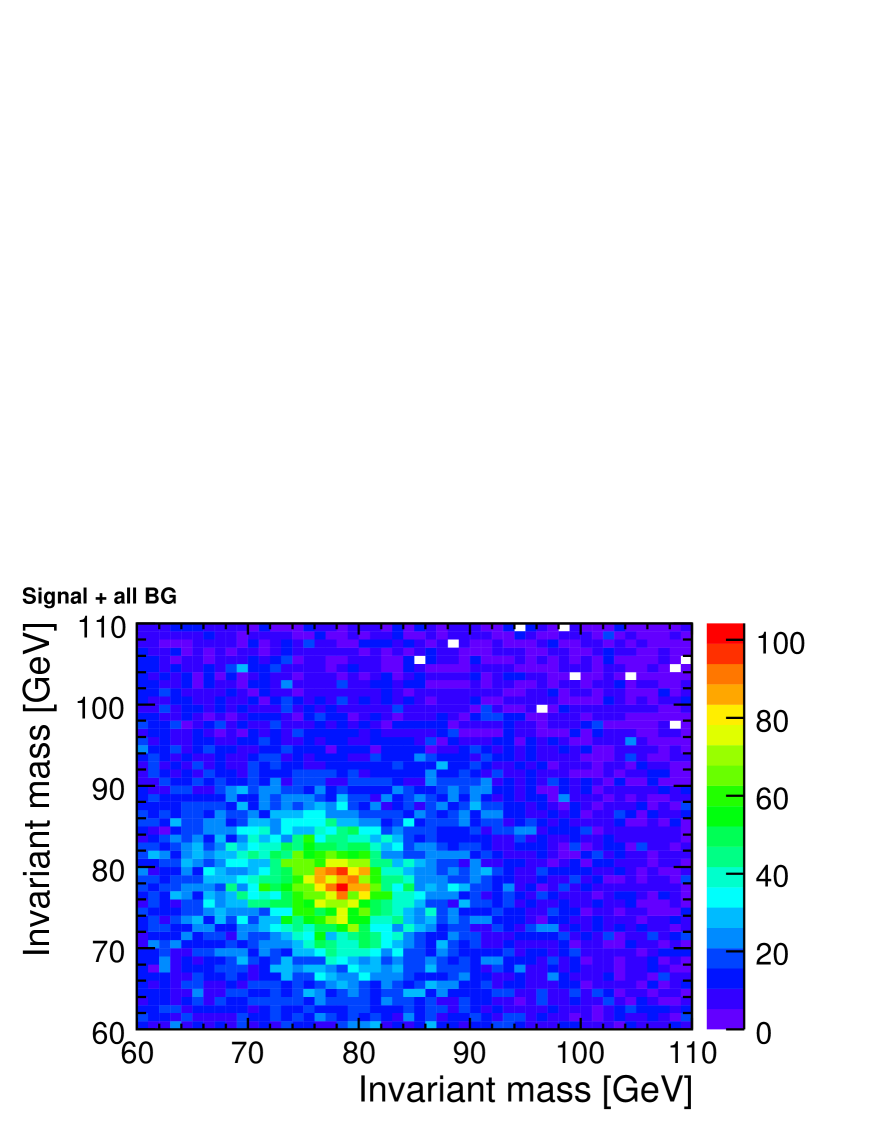
(a) All events (Sig + BG).

(c) Chargino-pair template (including all W decay mode).

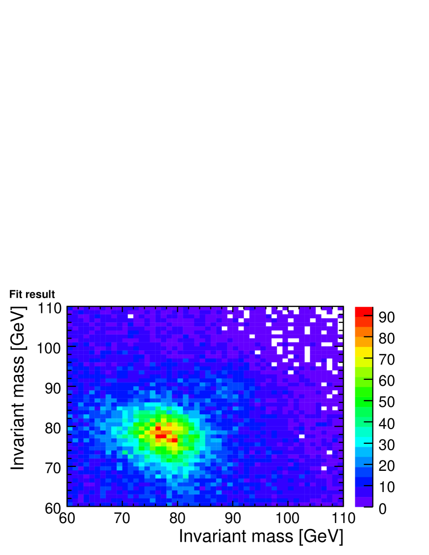
(e) Fit result to (a) - (b) with SM subtraction fluctuation.

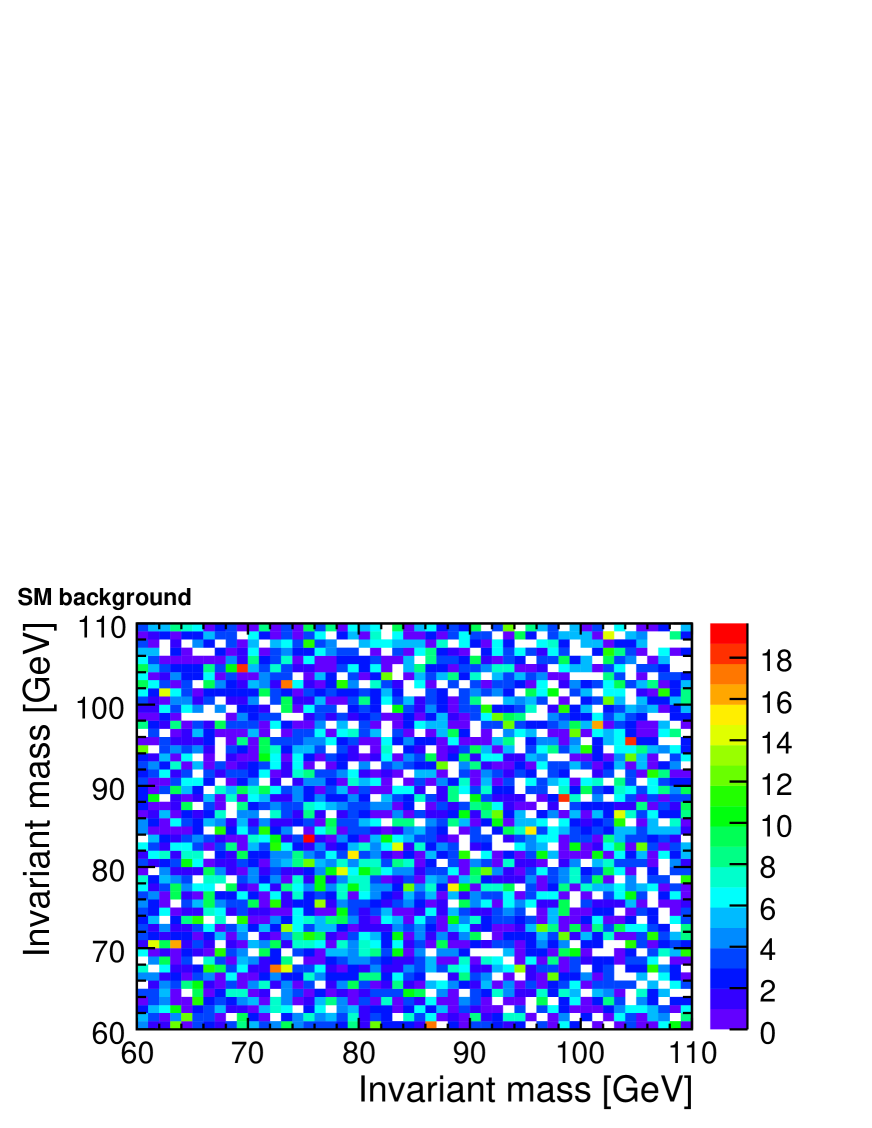
(b) SM background.

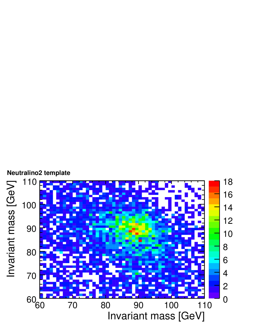
(d) Neutralino2-pair template (including all Z decay mode).

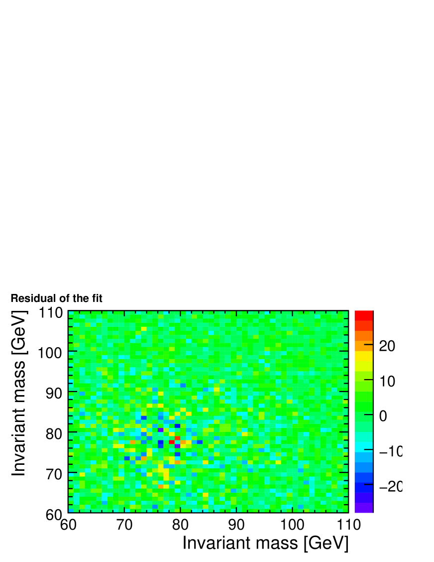
(f) Residual of the fit: (a) - (b) - (e).

Figure 4: Dijet mass distribution for cross-section fit. For (a) and (b) the same events are used, while (c) and (d) are statistically independent of (a).

Figure 4 shows the dijet mass distributions without the kinematic fit. All three possible jet-boson associations are taken into account in the histograms. 4a shows the dijet mass distribution of all Standard Model and SUSY point5 events passing the selection cuts; 4b is the SM part of 4a; 4c and 4d are statistically independent template samples for $\tilde{\chi}^{\pm}_{1}$ and $\tilde{\chi}^{0}_{2}$, made by 500 fb^-1. Before the fitting, the SM contribution (4b) is subtracted from the distribution of all events (4a). SUSY contributions other than $\tilde{\chi}^{\pm}_{1}$ and $\tilde{\chi}^{0}_{2}$ pair are not corrected for, but the contribution is negligibly small.

Figure 4e shows the result of a fit using a linear combination of the Chargino and Neutralino template distributions depicted 4c and d in. The residuals of the fit are displayed in figure 4f. They are sufficiently small and don’t show any specific structures, indicating a well working fit.

While it can be assumed that the SM distribution is well known and can be controlled for instance with the SM selection above, the assumption that the shape of the Chargino and Neutralino spectra is known is not evident. However, the shape of the dijet mass distribution on generator level is quite independent of the details of the SUSY scenario, as long as the decay into real $W$ and $Z$ bosons is open. As discussed already in section 3.2, the shape of the reconstructed dijet mass distribution is influenced by the mass differences between $\tilde{\chi}^{\pm}_{1}$ / $\tilde{\chi}^{0}_{2}$ and the LSP, which determines the boost of the vector bosons and thus has an effect on the amount of combinatorical background and the mass resolution. As shown in the next section, the masses of the gauginos can be measured purely from edge positions in the energy spectra of the gauge bosons, without any assumption on the cross-section. Thus, with the gaugino masses measured, we are confident that enough is known about the SUSY scenario at hand to apply the template method.

The background subtraction and the fit have been performed 10000 times, varying the bin contents of the SUSY and the SM distribution according to their statistical errors. The fitted fractions of Chargino and Neutralino contribution have been averaged over all fit outcomes, while the expected uncertainty is estimated from the variance of the fit results. Expressed in percent of the expected cross-section, this procedure yields $99.97\pm 0.84$% for the Chargino and $97.50\pm 2.75$% for the Neutralino case. In terms of absolute cross-sections this is equivalent to $\sigma(e^{+}e^{-}\rightarrow\tilde{\chi}^{+}_{1}\tilde{\chi}^{-}_{1})=124.80\pm 1.05$fb^-1 (MC: 124.84 fb^-1), and $\sigma(\sigma(e^{+}e^{-}\rightarrow\tilde{\chi}^{0}_{2}\tilde{\chi}^{0}_{2})=21.90\pm 0.62$fb^-1 (MC: 22.46 fb^-1).

If we use a best jet pairing rather than all combinations for the dijet mass, the statistical error grows by about 10%. This illustrates the fact that the true jet-boson association cannot always be found and that the jet pairings not classified as “best” still contain valuable information.

5 Mass Measurement

The masses of gauginos can be obtained via the energy spectrum of the $W$ and $Z$ boson candidates, since the distribution of gauginos is box-like with edges determined by the masses and the center-of-mass energy. Deviations from the pure box shape are due to the finite width of the $W$ and $Z$ bosons, the beam energy spectrum and the detector resolution. For the mass measurement, we have to separate the sample on an event-by-events basis into $\tilde{\chi}^{\pm}_{1}$ and $\tilde{\chi}^{0}_{2}$ pair candidates. This is done via the dijet masses, as described in the next subsection. Afterwards, the edge positions are fitted for both the Chargino and Neutralino selected sample. Finally, the actual masses are calculated from the edge positions.

5.1 Dijet Selection

For each event, the jet pairing with the highest probability in the kinematic fit is chosen. An event is selected as a Chargino or Neutralino candidate using the following $\chi^{2}$ variables, which are constructed from the invariant masses calculated from the four-vectors before the kinematic fit:

$$\chi^{2}_{W}(m_{1},m_{2}) = \frac{(m_{1}-m_{W})^{2}+(m_{2}-m_{W})^{2}}{\sigma^{2}}$$ (4)

$$\chi^{2}_{Z}(m_{1},m_{2}) = \frac{(m_{1}-m_{Z})^{2}+(m_{2}-m_{Z})^{2}}{\sigma^{2}},$$ (5)

where $m_{1}$ and $m_{2}$ are dijet masses of selected jet-pairs, $m_{W}$ and $m_{Z}$ are the nominal $W$ and $Z$ pole masses and $\sigma$= 5 GeV. Events with $\chi^{2}_{W}<4$ are classified as $\tilde{\chi}^{\pm}$, while events with $\chi^{2}_{W}>4$ & $\chi^{2}_{Z}<4$ are selected as $\tilde{\chi}^{0}_{2}$.

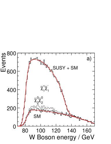
Figure 5: Mass determination: a) Energy spectrum of the $W^{\pm}$ candidates reconstructed from events selected as $\tilde{\chi}^{\pm}_{1}$ pairs and b) Energy spectrum of the $Z^{0}$ candidates reconstructed from events selected as $\tilde{\chi}^{0}_{2}$ pairs. In both cases, the Standard Model contribution has been fitted seperately before fitting the total spectrum.

Figure 5a) shows the energy spectrum of the selected $W$ candidates, while figure 5b) presents the same spectrum for the $Z$ candidates. The edge positions can be seen in the spectra, although the four-fermion background is still large, especially in the $Z$ energy distribution. The SM background can be fitted separately, as described below.

5.2 Fitting the Edges

In the next step, the energy spectra of the $W$ and $Z$ candidates are fitted according to the following procedure.

1. First, the Standard Model contribution is fitted with the following function:

   $$f_{SM}(x;t_{0},a_{0-2},\sigma,\Gamma)=\int^{\infty}_{t_{0}}(a_{2}t^{2}+a_{1}t+a_{0})V(t-x,\sigma,\Gamma)dt$$ (6)

   Here, $x$ denotes the boson energy, and $V(x,\sigma,\Gamma)$ is the Voigt function, i.e. a Breit-Wigner function of width $\Gamma$ convoluted with a Gaussian of resolution $\sigma$. The $t_{0}$ parameter adjusts the threshold position, while the parameters $a_{0}$, $a_{1}$ and $a_{2}$ are used to describe the shape of the plateau with a second order polynomial. The result of this fit is shown in figure 5.

2. Since the available statistics of the Standard Model sample is limited, the actual background used in the SUSY fit is generated from the fitted functions, including fluctuations according to the statistical errors expected from 500 fb^-1 of integrated luminosity.

3. Finally, the sum of the SUSY spectra and the SM spectra generated in the previous step are fitted. The SUSY part of the fitting function is similar to the one used on the Standard Model, but this time also an upper edge position $t_{1}$ is introduced. Furthermore, the Gaussian resolution $\sigma$ is allowed to have two different values at the edge positions, namely $\sigma_{0}$ and $\sigma_{1}$, with intermediate values obtained by linear interpolation.

   $$f(x;t_{0-1},b_{0-2},\sigma_{0-1},\Gamma) = f_{SM}+\int^{t_{1}}_{t_{0}}(b_{2}t^{2}+b_{1}t+b_{0})V(t-x,\sigma(t),\Gamma)dt$$ (7)

   $$\sigma(t;\sigma_{0},\sigma_{1}) = \sigma_{0}+\frac{(\sigma_{1}-\sigma_{0})(t-80)}{40}.$$ (8)

   All parameters of $f_{SM}$ are fixed to the values obtained in the first step. For the $\tilde{\chi}^{0}_{2}$ fit, $b_{2}$ is also fixed to 0.

Figure 5 shows the results of the SM fit as well as the results of SUSY mass fit for both the Chargino and the Neutralino selection.

To obtain edge positions, the fit is performed 100 times with different Standard Model spectra generated from the SM fit function. As final result, the averaged edge position and error are given:

• $\tilde{\chi}^{\pm}_{1}$ lower edge: $79.88\pm 0.19$ (MC: 79.80) GeV,

• $\tilde{\chi}^{\pm}_{1}$ upper edge: $131.49\pm 0.74$ (MC: 132.77) GeV,

• $\tilde{\chi}^{0}_{2}$ lower edge: $92.34\pm 0.44$ (MC: 93.09) GeV, and

• $\tilde{\chi}^{0}_{2}$ upper edge: $127.67\pm 0.76$ (MC: 129.92) GeV.

There is a tendency that the fitted numbers are slightly smaller than MC numbers. Better jet energy correction or modification of the fitting function can reduce the shift, but principally the shift could be corrected with a dedicated MC study.

5.3 Mass Determination from Edge Positions

The relation between the gaugino masses and the energy endpoints of the gauge bosons is determined by pure kinematics. Neglecting radiation losses, the energy of the gauginos is equal to the beam energy:$E_{\chi}=E_{\mathrm{beam}}$. In the gaugino restsystem, denoted with ^∗, the energy of the vector boson (i.e. $W$ or $Z$) is given by the usual formula for two-body decays:

$$E_{V}^{\ast}=\frac{M_{\chi}^{2}+M_{V}^{2}-M_{\mathrm{LSP}}^{2}}{2\cdot M_{\chi}},$$ (9)

where subscript $\chi$ denotes the decaying gaugino (i.e. $\tilde{\chi}^{\pm}_{1}$ or $\tilde{\chi}^{0}_{2}$), $V$ the vector boson (i.e. $W$ or $Z$) and the LSP $\tilde{\chi}^{0}_{1}$. Boosting this into the laboratory system yields:

$$E_{V}=\gamma E_{V}^{\ast}\pm\gamma\beta\sqrt{E_{V}^{\ast 2}-M_{V}^{2}}$$ (10)

The Lorentz boost $\gamma$ is given by $\gamma=E_{\chi}/M_{\chi}$, and $\beta=\sqrt{1-1/\gamma^{2}}$. The plus sign will give the upper edge of the allowed energy range, $E_{+}$, and the minus sign the lower one, $E_{-}$. For further calculations it is useful to introduce the center point of the allowed energy range, $E_{M}$, and its width $E_{D}$:

$$E_{M}=\frac{E_{+}+E_{-}}{2},\quad E_{D}=\frac{E_{+}-E_{-}}{2}$$ (11)

In solving equation 10 for the gaugino masses, it is useful to note that $\gamma\cdot E_{V}^{\ast}=E_{M}$. With this relation, $E_{V}^{\ast}$ can be eliminated and thus the LSP mass in obtained from $E_{D}$:

$$E_{D} = \gamma\sqrt{1-1/\gamma^{2}}\sqrt{E_{V}^{\ast 2}-M_{V}^{2}}$$ (12)

$$= \sqrt{1-1/\gamma^{2}}\sqrt{\gamma^{2}\cdot E_{V}^{\ast 2}-\gamma^{2}\cdot M_{V}^{2}}$$ (13)

$$= \sqrt{1-1/\gamma^{2}}\sqrt{E_{M}^{2}-\gamma^{2}\cdot M_{V}^{2}}$$ (14)

This is a quadratic equation in $\gamma^{2}$, which has two solutions:

$$\gamma^{2}=\frac{1}{2\cdot M_{V}^{2}}\left[(E_{+}\cdot E_{-}+M_{V}^{2})\pm\sqrt{(E_{+}^{2}-M_{V}^{2})(E_{-}^{2}-M_{V}^{2})}\right]$$ (15)

Inserting this into $\gamma\cdot E_{V}^{\ast}=E_{M}$, the LSP mass can be solved for:

$$M_{\mathrm{LSP}}^{2}=M_{V}^{2}+\frac{E_{\mathrm{beam}}^{2}}{\gamma^{2}}\left(1-\frac{E_{+}+E_{-}}{E_{\mathrm{beam}}}\right)$$ (16)

For a single energy spectrum, we thus have two solutions in the general case. However with the constraint that the LSP mass has to be the same for both the Chargino and the Neutralino decay, a unique solution can be determined - in this case the one with the upper sign.

For the point5 SUSY parameters, the lower edge of the $W$ energy spectrum is just equal to the $W$ rest mass, meaning that the $W$ bosons from the decay can be produced at rest, with the LSP carrying away all the momentum. This case has to be distinguished from a configuration where the boost is so large that the $W$ could actually fly into the same direction as the LSP in the laboratory frame. In this case, since the energy cannot become lower than the $W$ rest mass, the lower part of the spectrum would be “folded over” and create a second falling edge above the $W$ mass, precisely at $E_{V}=\sqrt{M_{V}^{2}+p_{V,\mathrm{min}}^{2}}$, where $p_{V,\mathrm{min}}=-\gamma\beta E_{V}^{\ast}+\gamma\sqrt{E_{V}^{\ast 2}-M_{V}^{2}}$. Moreover, this case of $E_{-}=M_{W}$ corresponds to the case where the equation for $\gamma^{2}$ has only one solution, with the $\pm$ term of equation 15 vanishing. At this point, the partial derivative $\partial E_{-}/\partial M_{\tilde{\chi}^{\pm}_{1}}$ becomes zero. So the inverse derivative which appears in the error propagation becomes undefined - or more realistically, with $E_{-}=M_{W}$ not exactly fulfilled, at least very large.

Since the discrimination between models is beyond the scope of this paper, but will be subject of future studies, we ignore here possible information from the lower edge of the $W$ energy spectrum. Instead, the lower and upper edge of the $Z$ energy spectrum are used to calculate the masses of $\tilde{\chi}^{0}_{2}$ and $\tilde{\chi}^{0}_{1}$. In a second step, the Chargino mass is calculated from the LSP mass and the upper edge of the $W$ spectrum.

The error propagation is done by using a toy Monte Carlo, taking into account the correlations between the two masses determined from one energy spectrum. It calculates the gaugino masses by above equations with edge positions varying randomly according to their errors obtained from the edge fit. For the center edge positions two patterns were tried, the fitted edge positions and the MC truth positions.

Table 3 shows the obtained mass values and errors. Without correction of the edge position, the average value of obtained masses deviates by 3-4 GeV from the MC truth. This might be due to the fact that phase space was not considered, and could be reduced by an improved fitting function. with better fitting functions. Without the kinematic fit, the mass resolution is worse by typically 400 to 500 MeV, which corresponds to 15 to 40% of the errors, depending on the gaugino considered.

6 Summary

The physics performance of the ILD detector concept has been evaluated using a SUSY benchmark scenario referred to as “Point 5”, where $\tilde{\chi}^{\pm}_{1}$ and $\tilde{\chi}^{0}_{2}$ are nearly mass degenerate and decay into real $W^{\pm}$ and $Z^{0}$ bosons, respectively, plus a $\tilde{\chi}^{0}_{1}$. The cross-sections for Chargino and Neutralino pair production have been obtained by a fit to the two-dimensional dijet mass spectrum relying on Monte-Carlo templates. The resulting statistical errors are 0.84% in the Chargino case and 2.75% in the Neutralino case.

The gaugino masses have been determined from a fit to the edges of the energy spectra of the $W^{\pm}$ and $Z^{0}$ bosons obtained by a kinematic fit. The resulting mass resolutions are 2.9 GeV, 1.7 GeV and 1.0 GeV for $\tilde{\chi}^{\pm}_{1}$, $\tilde{\chi}^{0}_{2}$ and $\tilde{\chi}^{0}_{1}$, respectively. Without the kinematic fit, the mass resolution is worse by 400 to 500 MeV.

	$\tilde{\chi}^{+}_{1}\tilde{\chi}^{-}_{1}\rightarrow$ hadrons	$\tilde{\chi}^{0}_{2}\tilde{\chi}^{0}_{2}\rightarrow$ hadrons	other SUSY	SM $\gamma\gamma$	SM 6f	SM 4f	SM 2f
nocut	28529	5488	74650	3.66e+09	521610	1.48e+07	2.14e+07
Total # of tracks $\geq 20$	27897	5449	24305	3.03e+06	495605	6.68e+06	5.33e+06
$100<E_{\mathrm{vis}}<300$ GeV	27895	5449	22508	1.06e+06	44394	959805	1.56e+06
$E_{\mathrm{jet}}>5$	27889	5446	20721	908492	44096	916507	1.47e+06
$|\cos(\theta)_{\mathrm{jets}}|<0.99$	26560	5240	19200	350364	41098	678083	874907
$y_{34}>0.001$	26416	5218	15255	202510	38638	423080	166305
# of tracks $\geq 2/$jets	25717	5146	9559	162193	22740	255870	145270
$|\cos{\theta_{\mathrm{miss}}}|<0.99$	25463	5099	9487	25087	22311	193706	4039
$E_{\mathrm{l}}<25$	25123	4981	6463	23133	14407	154927	3534
$N_{\mathrm{PFO}}>3$	25029	4975	6103	23014	13696	139429	3518
$|\cos{\theta_{\mathrm{miss}}}|<0.8$	20144	4079	5180	681	9950	62668	529
$M_{\mathrm{miss}}>220$ GeV	20139	4079	5180	630	3687	45867	389
kin. fit converged	20085	4068	4999	626	3649	44577	341

Table 1: Event numbers after each of the selection cuts, normalized to 500 fb^-1 and $P(e^{+},e^{-})=(30\%,-80\%)$.

Processes	No cut	all cuts	Purity	Efficiency
$\tilde{\chi}^{+}_{1}\tilde{\chi}^{-}_{1}\rightarrow$ hadrons	28529	16552	58%	58%
$\tilde{\chi}^{0}_{2}\tilde{\chi}^{0}_{2}\rightarrow$ hadrons	5488	3607	13%	65%
Other SUSY point5	74650	77	0.27%	$1.0\times 10^{-3}$
qqqq (WW, ZZ)	4.29e+06	5885	21%	$1.4\times 10^{-3}$
qq$\ell\nu$ (WW)	5.19e+06	561	2.0%	$1.1\times 10^{-4}$
qqqq$\ell\nu$ (tt)	216996	489	1.7%	$2.3\times 10^{-3}$
$\gamma\gamma\rightarrow$qqqq	26356	397	1.4%	1.5%
qqqq$\nu\nu$ (WWZ)	9262	268	0.94%	2.9%
qq$\nu\nu$ (ZZ)	367779	76	0.27%	$2.1\times 10^{-4}$
qq	9.77e+06	76	0.27%	$7.8\times 10^{-6}$
Other background	3.68e+09	438	1.5%	$1.2\times 10^{-7}$

Table 2: Purity and efficiency of signal and major background sources after the selection cuts and with an invariant dijet mass larger than 65 GeV. The processes in pathentheses indicate the dominant intermediate states.

Observables	Obtained value	Error	Error at the true mass
$m(\tilde{\chi}^{\pm}_{1})$	220.90 GeV	2.90 GeV	3.34 GeV
$m(\tilde{\chi}^{0}_{2})$	220.56 GeV	1.72 GeV	1.39 GeV
$m(\tilde{\chi}^{0}_{1})$	118.97 GeV	1.02 GeV	0.95 GeV

Table 3: Performance on gaugino masses and associated errors. The last column shows errors on masses when the true edge positions are used in the error propagation. MC truth masses are 216.7, 216.5 and 115.7 GeV for $\tilde{\chi}^{\pm}_{1}$, $\tilde{\chi}^{0}_{2}$ and $\tilde{\chi}^{0}_{1}$, respectively.

Figure 2: Dijet mass spectrum for Standard Model selection. The event sample is dominated by 4-fermion events, with a small contribution from 6-fermion events, but doesn’t contain any SUSY events.

References

- [1] M. Battaglia et al., “Physics benchmarks for the ILC detectors,” In the Proceedings of 2005 International Linear Collider Workshop (LCWS 2005), Stanford, California, 18-22 Mar 2005, pp 1602 [arXiv:hep-ex/0603010].
- [2] W. Porod, “SPheno, a program for calculating supersymmetric spectra, SUSY particle decays and SUSY particle production at colliders,” Comput. Phys. Commun. 153 (2003) 275 [arXiv:hep-ph/0301101].
- [3] S. Agostinelli et al. [GEANT4 Collaboration], “GEANT4: A simulation toolkit,” Nucl. Instrum. Meth. A 506 (2003) 250.
- [4] ILD Concept Group, “The International Large Detector — Letter of Intent,” DESY-09-087, http://www.ilcild.org/documents/ild-letter-of-intent
- [5] M. A. Thomson, “Particle flow calorimetry at the ILC,” AIP Conf. Proc. 896, 215 (2007).
- [6] W. Kilian, T. Ohl and J. Reuter, “WHIZARD: Simulating Multi-Particle Processes at LHC and ILC,” arXiv:0708.4233 [hep-ph].
- [7] O. Wendt, F. Gaede and T. Kramer, “Event reconstruction with MarlinReco at the ILC,” Pramana 69 (2007) 1109 [arXiv:physics/0702171].
-
[8]
B. List, J. List,
“MarlinKinfit: An Object–Oriented Kinematic Fitting Package,”
LC-TOOL-2009-001, http://www-flc.desy.de/lcnotes/