Low-Prandtl-number Bénard-Marangoni convection in a vertical magnetic field

Abstract

The effect of a homogeneous magnetic field on surface-tension-driven Bénard convection is studied by means of direct numerical simulations. The flow is computed in a rectangular domain with periodic horizontal boundary conditions and the free-slip condition on the bottom wall using a pseudospectral Fourier-Chebyshev discretization. Deformations of the free surface are neglected. Two- and three-dimensional flows are computed for either vanishing or small Prandtl number, which are typical of liquid metals. The main focus of the paper is on a qualitative comparison of the flow states with the non-magnetic case, and on the effects associated with the possible near-cancellation of the nonlinear and pressure terms in the momentum equations for two-dimensional rolls. In the three-dimensional case, the transition from a stationary hexagonal pattern at the onset of convection to three-dimensional time-dependent convection is explored by a series of simulations at zero Prandtl number.

I Introduction

Bénard-Marangoni convection (BMC) in a plane fluid layer with an open surface is the surface-tension-driven analog to buoyancy-driven Rayleigh-Bénard convection (RBC) in a layer with rigid top and bottom walls. Both systems present classic examples of hydrodynamic instabilities, and are generic models for convective flows driven by buoyancy and Marangoni forces, respectively.

Many works on BMC are devoted to the regular cellular patterns as dissipative structures, which are observed in highly viscous fluids such as silicone oils, e.g. Bestehorn (1993); Golovin et al. (1997); VanHook et al. (1997); Eckert et al. (1998). In these experimental and theoretical investigations, BMC is either stationary or only weakly time-dependent, and the Prandtl number $P$ is large compared with unity because of the high kinematic viscosity.

Marangoni convection in low Prandtl number fluids, i.e. liquid metals or semiconductor melts (with $P$ of order $10^{-2}$), plays an important role in industrial processes such as crystal growth Davis (1987) or electron beam evaporation Pumir and Blumenfeld (1996). Theoretical and experimental studies as well as numerical simulations have therefore been largely focused on configurations resembling actual industrial setups such as the floating zone Kuhlmann and Rath (1993); Levenstam and Amberg (1995).

By contrast, BMC in liquid metals has received comparatively little attention. The only experimental work known to the author is the study of Ginde et al. Ginde et al. (1989), where liquid tin was used. Theoretical studies of Dauby et al. Dauby et al. (1993) and of Thess & Bestehorn Thess and Bestehorn (1995) predict the occurrence of “inverted” hexagons at the onset of convection for sufficiently small Prandtl numbers. The orientation of the flow in such hexagonal cells is opposite to that found at high Prandtl numbers.

Numerical studies of two- and three-dimensional BMC were undertaken by the present author in collaboration with A. Thess Boeck and Thess (1997, 1998, 1999). In Boeck and Thess (1997, 1999), partiulcar attention was paid to the limit of vanishing Prandtl number. Earlier studies of RBC had already explored low Prandtl numbers, and noted interesting behavior of two-dimensional roll solutions, termed inertial convection Proctor (1977); Busse and Clever (1981). The analog of inertial convection in RBC was observed and analyzed in Boeck and Thess (1997) for BMC. This type of convection is characterized by the dominance of inertia over viscous forces and a low energy dissipation. However, the two-dimensional rolls are susceptible to three-dimensional perturbations, and inertial convection is therefore typically not realized in three-dimensional simulations Thual (1992); Boeck and Thess (1999). Some indications for the existence of inertial convection come from RBC experiments with mercury and sodium Chiffaudel et al. (1987); Kek and Müller (1993), but those are only based on integral heat flux measurements for a narrow range of Prandtl numbers.

In contrast to the non-conducting high-Prandtl-number liquids, the Bénard-Marangoni instability in liquid metals can be influenced by magnetic fields. For a vertical applied field the linear stability theory has been thoroughly explored by several authors Nield (1966); Wilson (1993, 1994); Thess and Nitschke (1995); Hashim and Wilson (1999). In this configuration the magnetic field does not introduce horizontal anisotropy. The magnetic field suppresses the instability, i.e., the necessary temperature difference for convective instability grows with the magnetic induction $B$. For sufficiently strong $B$, the vertical structure of the unstable mode exhibits Hartmann layers at the bottom and the free surface, and the corresponding critical wavelength shrinks Thess and Nitschke (1995).

A horizontal component of the magnetic field introduces horizontal anisotropy, but would not suppress the instability because the roll axis of the normal mode can always be aligned with the field. In this case no Lorentz force is produced. The resulting anisotropy of the flow pattern has been discussed in the context of linear theory Thess and Nitschke (18-22 November 1991), but not on the basis of nonlinear simulations.

The nonlinear behavior with a vertical magnetic field has so far only been examined using perturbation methods, which only apply near the onset of convection Miladinova and Slavtchev (2001). The present paper continues the investigations of nonlinear BMC with a vertical magnetic field using the direct simulation approach of Boeck and Thess (1997, 1999), whereby large Marangoni numbers and complex flows can be realized numerically. Both two- and three-dimensional simulations will be performed in order to analyze the qualitative effects of the magnetic field on the particular solutions described in Boeck and Thess (1997, 1999). The choice of parameters and boundary conditions is therefore guided by these previous works.

The paper is organized as follows. In the following section the basic equations and the numerical method will be described. After that, the two-dimensional and three-dimensional simulation results are presented and analyzed in separate sections. The paper ends with some conclusions and suggestions for future work.

II Basic equations and numerical method

The system under study is a planar liquid layer of thickness $d$ with a free upper surface, which is heated from below. The liquid has a finite electric conductivity $\sigma$. Buoyancy and surface deflections are neglected. The isothermal bottom of the layer is located at $z=0$ and the free surface at $z=d$. Periodic boundary conditions apply in the $x$- and $y$-directions. The thickness $d$ is chosen as lengthscale for non-dimensionalization. The dimensionless quantities $L_{x}$ and $L_{y}$ denote the periodicity length with respect to $x$ and $y$.

As in Boeck and Thess (1997), free-slip conditions are assumed at the bottom of the layer in order to compare with the non-magnetic case. The heat flux density at the free surface is assumed fixed in the present work, which corresponds to the limit of zero Biot number. It is convenient to introduce the deviation $\theta$ from the the conductive temperature profile by writing

$$T=\theta+T_{b}-\Delta T_{0}z/d.$$ (1)

Here $T_{b}$ is the prescribed bottom temperature and $\Delta T_{0}$ the conductive temperature difference. Notice that $\theta(x,y,z)\leq\Delta T_{0}z/d$ since the fluid cannot become hotter than the bottom wall. The shear stresses at the free surface are

$$\rho\nu\frac{\partial\bm{v}}{\partial z}=\nabla\Sigma=-\gamma\nabla T,$$ (2)

where the coefficient $\gamma$ characterizes the linear decrease in surface tension $\Sigma$ with temperature. The symbols $\bm{v}$, $\rho$ and $\nu$ are the fluid velocity, density and kinematic viscosity. The vectors in eq. (2) are understood to be projected onto the free surface.

The Lorentz force and the induced current due to the external homogeneous magnetic field $B$ will be treated in the limit of low magnetic Reynolds number. As explained in Davidson (2001), this approximation is justified for length scales and velocities realized in the laboratory and in industrial applications. It takes into account the action of the magnetic field on the velocity field but ignores the reaction of the flow on the magnetic field. The densities of induced current and Lorentz force in this approximation are given by

$$\bm{j}=\sigma\left(-\nabla\phi+\bm{v}\times\bm{B}\right),\hskip 8.53581pt\bm{f}=\bm{j}\times\bm{B}.$$ (3)

The divergence of the induced current density $\bm{j}$ vanishes because of the extremly short charge relaxation time in comparison with the time scales of magnetohydrodynamic flows (Davidson, 2001, Section 2.2). For this reason, the electric potential $\phi$ satisfies

$$\nabla^{2}\phi=\nabla\cdot\left(\bm{v}\times\bm{B}\right).$$ (4)

It is also assumed that the liquid is bounded by electrical insulators, i.e. the normal component $j_{z}$ of the current density vanishes at the top and the bottom of the layer. Using Ohm’s law, $j_{z}=0$ translates into boundary conditions on $\phi$.

The equations will be given in a form based on viscous velocity scaling, i.e. $\nu/d$ is the velocity scale and $d^{2}/\nu$ the time scale. Furthermore, $\nu\Delta T_{0}/\kappa$ serves as scale of $\theta$, where $\kappa$ denotes the thermal diffusivity of the fluid. The magnetic field is oriented in along the $\bm{e}_{z}$ unit vector, and the scale of the electric potential is given by $B\nu$. The dimensionless equations are

$$\frac{\partial\bm{v}}{\partial t}+(\bm{v}\cdot\nabla)\bm{v} = -\nabla p+\nabla^{2}\bm{v}+Ha^{2}\left(-\nabla\phi+\bm{v}\times\bm{e}_{z}\right)\times\bm{e}_{z},$$ (5)

$$\nabla\cdot\bm{v} = 0,$$ (6)

$$\nabla^{2}\phi = \nabla\cdot\left(\bm{v}\times\bm{e}_{z}\right),$$ (7)

$$P\left(\frac{\partial\theta}{\partial t}+(\bm{v}\cdot\nabla)\theta\right) = \nabla^{2}\theta+v_{z}.$$ (8)

At the bottom $z=0$, the conditions

$$\frac{\partial v_{x}}{\partial z}=\frac{\partial v_{y}}{\partial z}=v_{z}=\theta=\frac{\partial\phi}{\partial z}=0$$ (9)

apply. The boundary conditions at the top surface $z=1$ are

$$\frac{\partial v_{x}}{\partial z}+Ma\,\frac{\partial\theta}{\partial x}=\frac{\partial v_{y}}{\partial z}+Ma\,\frac{\partial\theta}{\partial y}=v_{z}=\frac{\partial\theta}{\partial z}=\frac{\partial\phi}{\partial z}=0$$ (10)

with the Marangoni number

$$Ma=\frac{\gamma\Delta T_{0}d}{\rho\nu\kappa}$$ (11)

as control parameter for the forcing. The remaining parameters are the Prandtl number $P=\nu/\kappa$ and the Hartmann number

$$Ha=Bd\sqrt{\frac{\sigma}{\rho\nu}}.$$ (12)

The scale for $\theta$ has been chosen in such a way that a coupling of velocity and temperature is maintained also in the limit $P=0$, i.e. when the left hand side in (8) vanishes. This approximation is called the (viscous) zero–Prandtl–number limit. The same limit has been considered in the work of Thual Thual (1992) for RBC. Other limiting cases based on different temperature and velocity scalings are also discussed in this work, and it is argued that these other cases either do not provide a uniform approximation throughout the fluid domain, or model transients or flows where thermal convection is merely a side effect.

Convective heat transport is measured by the nondimensional Nusselt number $Nu$ defined as the ratio between the total heat flux and the conductive heat flux. In contrast to convection between isothermal plates with fixed temperatures, convection reduces the temperature drop across the layer. Since the contribution of heat conduction to the total heat transport is thereby reduced, one has to compute the conductive heat flux for the present, reduced surface temperature. The result reads

$$Nu=\frac{1}{1-P\langle\theta_{s}\rangle},$$ (13)

where

$$\langle\theta_{s}\rangle=\frac{1}{L_{x}L_{y}}\int_{0}^{L_{x}}\int_{0}^{L_{y}}\theta(x,y,1)d\,x\,d\,y$$ (14)

denotes the mean perturbation of the surface temperature.

In the zero–Prandtl–number limit $Nu$ equals unity. Results for $P>0$ can be extrapolated from $P=0$ if one regards the solution of the zero–Prandtl–number equations as the leading term in an expansion in $P$. The calculations given in Boeck and Thess (1997) lead to the following results for mean surface temperature perturbation $\langle\theta_{s}\rangle$ and $Nu-1$:

$$\langle\theta_{s}\rangle = P\int_{0}^{1}\langle v_{z}\theta\rangle dz+O(P^{2}),$$ (15)

$$Nu-1 = P^{2}\int_{0}^{1}\langle v_{z}\theta\rangle dz+O(P^{3}).$$ (16)

In these equations, $v_{z}$ and $\theta$ are the solutions of the zero–Prandtl–number equations. Due to its connection with the Nusselt number the quantity $\overline{v_{z}\theta}$ (where the overbar symbol denotes the volume average) will be referred to as reduced Nusselt number.

Finally, the alternative scaling of the basic equations based on the units $\kappa/d$ for velocity, $\kappa B$ for the electric potential and $\Delta T_{0}$ for the temperature perturbation $\theta$ will be needed for later discussion. The equations (5-8) then take the form

$$\frac{\partial\bm{v}}{\partial t}+(\bm{v}\cdot\nabla)\bm{v} = -\nabla p+P\left[\nabla^{2}\bm{v}+Ha^{2}\left(-\nabla\phi+\bm{v}\times\bm{e}_{z}\right)\times\bm{e}_{z}\right],$$ (17)

$$\nabla\cdot\bm{v} = 0,$$ (18)

$$\nabla^{2}\phi = \nabla\cdot\left(\bm{v}\times\bm{e}_{z}\right),$$ (19)

$$\frac{\partial\theta}{\partial t}+(\bm{v}\cdot\nabla)\theta = \nabla^{2}\theta+v_{z}.$$ (20)

The boundary conditions (9,10) remain unchanged, but for the Nusselt number one has to use

$$Nu=\frac{1}{1-\langle\theta_{s}\rangle}$$ (21)

instead of (13).

The numerical code for two- and three-dimensional direct simulations is based on equations (5-8) and a pseudospectral Fourier-Chebyshev discretization. It has been described in Boeck and Thess (1999) for the non-magnetic case. The modifications for the present case with vertical magnetic field are analogous to the implementation of the electric potential and Lorentz force terms for the channel code discussed in Krasnov et al. (2004).

III Linear stability results

The linear stability of the basic conductive state has been treated in several papers, including asymptotic limits of large Hartmann number and Biot numbers as well as zero and finite crispation numbers Nield (1966); Wilson (1993, 1994); Thess and Nitschke (1995); Hashim and Wilson (1999). For the purposes of the present paper the critical Marangoni and wavenumbers for free-slip boundary conditions at the bottom are required as a function of the Hartmann number.

The velocity and temperature perturbations for the neutral stability problem are

$$v_{z}(x,z)=W(z)\exp\left(ikx\right),\hskip 14.22636pt\theta(x,z)=\Theta(z)\exp\left(ikx\right),$$ (22)

whereby one obtains the stability equations

$$\left[\left(D^{2}-k^{2}\right)^{2}+Ha^{2}D^{2}\right]W(z)=0,\hskip 14.22636pt\left[D^{2}-k^{2}\right]\Theta(z)=-W(z)$$ (23)

and the boundary conditions

$$W(0)=W(1)=\Theta(0)=D\Theta(1)=D^{2}W(0)=D^{2}W(1)+Ma\,k^{2}\,\Theta(1)=0.$$ (24)

The symbol $D$ denotes the $z$-derivative. Notice that the Prandtl number is absent from these equations since the neutral conditions are independent of $P$. Because of the linearity of the system (23-24), one can choose the normalization $D^{2}W(1)=1$ to solve these equations without the Marangoni boundary condition

$$Ma\,k^{2}\,\Theta(1)=-D^{2}W(1).$$ (25)

Eq. (25) is then used to calculate the Marangoni number $Ma(k)$ for neutral conditions at the chosen wavenumber $k$. The solution of the fourth-order equation for $W$ and the second-order equation for $\Theta$ is obtained simultaenously by a Chebyshev collocation method.

Critical conditions are found by searching for the minimum $Ma(k)$ for the given value of $Ha$, which provides the critical parameters $Ma_{c}(Ha)$ and $k_{c}(Ha)$. The results are shown in Fig. 1 for free-slip ($D^{2}W(0)=0$) and no-slip ($DW(0)=0$) boundary conditions at the bottom. The critical Marangoni and wavenumber are smaller for the free-slip case, but the difference vanishes as $Ha$ increases. The asymptotic relations

$$Ma_{c}\sim Ha^{2},\hskip 28.45274ptk_{c}\sim 0.7926\sqrt{Ha},$$ (26)

shown in Fig. 1 have been obtained by Wilson Wilson (1993) for the no-slip case and are discussed and interpreted by Thess & Nitschke Thess and Nitschke (1995). They appear to be valid irrespective of the bottom boundary condition on the velocity. The vertical structure of the neutral modes differs only in a zone of width $1/Ha$ at the bottom between the free- and no-slip cases. Near the free surface, the unstable modes display a boundary layer structure with a width of order $1/Ha$ as explained in Thess and Nitschke (1995).

(a)

(b)

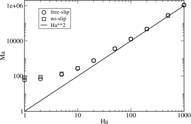
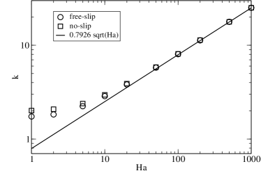
Figure 1: Critical Marangoni and wavenumbers for neutral conditions.

IV Two-dimensional convection

IV.1 Transition from weak to inertial convection

(a)

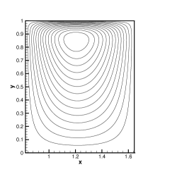
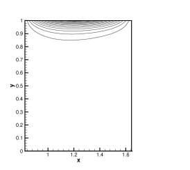
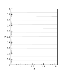
(b)

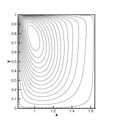
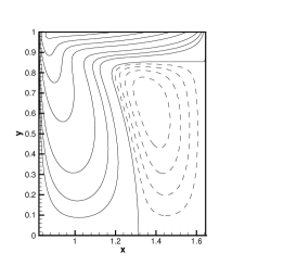
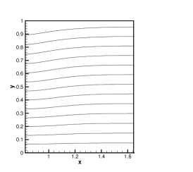
(c)

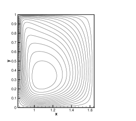
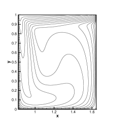
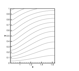
(d)

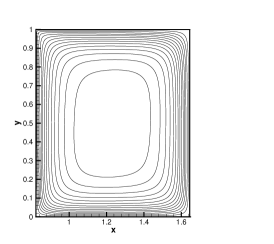
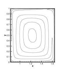
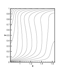
Figure 2: Isocontours of streamfunction (left column), vorticity (middle column) and temperature (right column) of steady two-dimensional convection with $Ha=20$, $P=0.02$, $L_{x}=2\pi/k_{c}$. Only a single roll is shown due to the imposed mirror symmetry. The flow orientation is counter-clockwise. (a) corresponds to $Ma=758$, (b) to $Ma=1000$, (c) to $Ma=2000$, (d) to $Ma=32000$.

Two-dimensional solutions will be considered first as they display several interesting features in the non-magnetic case Boeck and Thess (1997). In particular, large Marangoni numbers can be explored more easily than in three-dimensional simulations. The computational domains are chosen on the basis of the linear stability analysis in the previous section for Hartmann numbers $Ha=10$ and $Ha=20$. For these values we have the critical parameters $Ma_{c}(Ha=10)=271.2$, $k_{c}(Ha=10)=2.87$ and $Ma_{c}(Ha=20)=757.2$, $k_{c}(Ha=20)=3.82$. The simulations are therefore performed with a periodicity length $L_{x}=2\pi/k_{c}$, where $k_{c}$ takes the value corresponding to $Ha=10$ and $Ha=20$. This way, two roll cells fit into the computational domain at the onset of convection, i.e. for $Ma_{c}$. In order to delay instabilities and to maintain this flow topology at larger values of $Ma$ the mirror symmetry between the rolls is enforced by the numerical method through symmetry conditions on the Fourier coefficients.

Simulation results are shown in Fig. 2 for $Ha=20$ and $Pr=0.02$ for several values of the Marangoni number. The simulations evolve to a steady flow in all cases shown. Near the onset of convection at $Ma=758$ nonlinear effects are weak, and the flow field reflects the structure of the neutrally stable mode associated with the critical Marangoni number. One can clearly identify the boundary layer at the free surface originating from the Lorentz force in the streamline pattern.

For $Ma=1000$ (Fig. 2(b)) the vorticity remains no longer confined near the free surface, but is swept into the bulk because of the stronger advection. A significant difference to the non-magnetic case is the change of sign of the vorticity in the domain indicated by the dashed isolines (middle column). This change of sign is an indication of the Lorentz force impeding the advection of vorticity in the bulk of the liquid layer. For larger values of $Ma$ the advection dominates and the negative vorticity region disappears. Moreover, the streamfunction and vorticity distributions become approximately symmetric with matching isolines near the center of the roll (Fig. 2(d)). In this case, the flow approaches an inviscid balance between pressure gradient and advection term in the bulk region since the gradients of streamfunction and vorticity become aligned. The viscous and Lorentz force terms are then weak by comparison with the other terms in the Navier-Stokes equation.

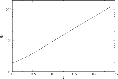
Figure 3: Spatial rms velocity in viscous units as function of time for two-dimensional BMC with $P=0$, $Ma=1350$ and $Ha=20$.

The tendency of the flow to approach such a nearly inviscid configuration has a profound consequence for the limit of vanishing Prandtl number. When the forcing of the flow by the surface tension gradients is strong enough to establish such a nearly inviscid balance, then the approximate cancellation of pressure and advection term imply that only the linear terms control the dynamics in the momentum equation (5). The forcing is provided by the Marangoni boundary condition coupling temperature perturbation and shear stress, and the temperature perturbation becomes a linear functional of the velocity field in the limit $P=0$ (eq. (8)). One can then expect the velocity to grow exponentially in time since the dynamics is governed by an effectively linear equation with a forcing term proportional to the velocity itself. This is illustrated by Fig. 3, which shows the growth of the mean velocity with time for $Ha=20$ and $Ma=1350$. The simulation was started from the steady solution for $P=0.005$ with the Prandtl number set to zero at $t=0$. After a short initial transient, the streamfuction and vorticity fields approach the symmetric state with an approximate inviscid balance similar to Fig. 2(d), and the spatial rms velocity grows exponentially with time. This behavior is completely analogous to the non-magnetic case Boeck and Thess (1997).

For finite Prandtl numbers, the unbounded growth of the velocity eventually stops since the temperature difference across the layer is reduced by the fast advection, and the shear stress diminishes because of the correspondingly reduced temperature difference on the free surface. Because the saturation of the velocity is provided by the heat transport it turns out that the appropriate scaling of the velocity and temperature are provided by thermal units $\kappa/d$ and $\Delta T_{0}$. If velocity and temperature perturbations are measured in these units, then these quantities become independent of $P$ for $P\to 0$, and equations (17-20) are appropriate. This mode of convection is the inertial convection mentioned in the introduction. Conversely, when the forcing by the surface-tension gradient is not too strong, then the velocity field does not attain the symmetric streamlines required for the approximate cancellation of pressure gradient and advection term, and the momentum transport is responsible for nonlinear saturation of the convective instability. In this case, the viscous units provide the appropriate scales for velocity and temperature perturbation in the limit $P\to 0$. This mode of convection has been termed weak convection in Ref.Boeck and Thess (1997).

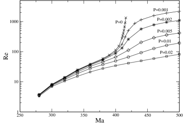
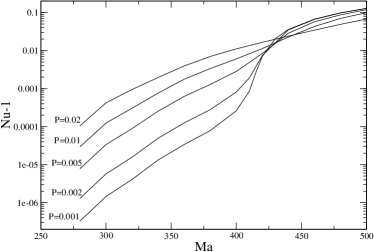
(b)

     

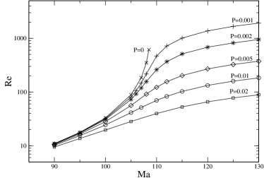
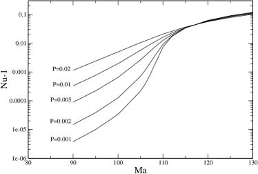
(c)

     

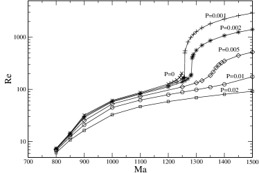
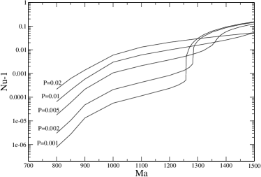
(d)

     

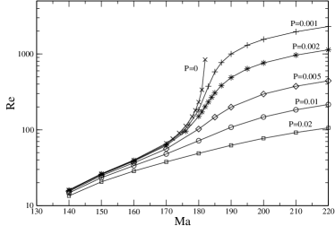
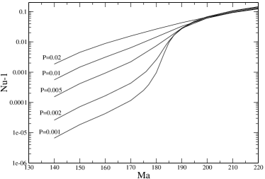
Figure 4: Reynolds and Nusselt numbers for steady two-dimensional BMC with $L_{x}=2\pi/k$. Cases (a,b) have $k=2.87$ and different values $Ha=10$ (a) and $Ha=0$ (b). Cases (c,d) have $k=3.82$ and different values $Ha=20$ (c) and $Ha=0$ (d).

The change from viscous to thermal scaling appears in a certain range of Marangoni numbers. Fig. 4 illustrates the switch from viscous to thermal scaling by the Reynolds number, i.e. the spatial rms velocity in viscous units, and the quantity $Nu-1$, which scales as $P^{2}$ when the viscous scaling applies, and which becomes independent of $P$ when the thermal scaling holds. The steady flows were computed for five finite values of the Prandtl number from $P=0.001$ up to $P=0.02$ and for $P=0$, and for $Ha=10$ and $Ha=20$ with the corresponding domain sizes $L_{x}=2\pi/k_{c}$. In addition, the computations were repeated for the non-magnetic case ($Ha=0$) with the same domain sizes $L_{x}=2\pi/k_{c}$ as for $Ha=10$ and $Ha=20$. The numerical resolution for the simulations was adjusted depending on the Reynolds number, and convergence was verified for several parameter sets by doubling the number of collocation points in both directions. Typical resolutions at the lowest value of $P$ were $N_{x}=1024$ and $N_{z}=129$ collocation points.

The left column of Fig.4 shows that the spatial rms velocity (Reynolds number) approaches the limiting curve for $P=0$ when the Marangoni number is not too large. When scaled in thermal units, the rms velocity would tend to zero as $P\to 0$, i.e. the curves would look similar to $Nu-1$ in the right column. For sufficiently large Marangoni numbers, the curves for $Nu-1$ show a tendency to converge onto a limiting curve as $P$ is reduced. The rms velocity of the steady solution branch for $P=0$ shows either a very rapid growth over a narrow $Ma$-range or appears to end abruptly for $Ha=20$. In the non-magnetic case there is an additional bifurcation in the $P=0$ solution branch Boeck and Thess (1997), which appears to be absent in the four combinations of $Ha$ and $L_{x}$ investigated here. This bifurcation allows one to clearly distinguish between the weak convection regime with viscous scaling for $P\to 0$ and the inertial regime with thermal scaling in the non-magnetic case Boeck and Thess (1997). In the present cases, the transition from weak to inertial convection at fixed $P$ is gradual except for $Ha=20$, where a discontinuity is present at sufficiently low $P$. Concerning the apparently different behaviors of the solution branches for $P=0$ one has to bear in mind that these cases are very hard to resolve numerically. The solutions converge very slowly, and are rather sensitive to the spatial resolution, which must be increased with the Reynolds number to resolve the increasingly smaller viscous boundary layers. The asymptotic behavior with $Ma$ of the branches with $P=0$ cannot be reliably determined in the present numerical approach.

The extensive computations summarized by Fig. 4 were performed for the non-magnetic and magnetic cases with the same periodicity length in order to quantify by how much the Lorentz forces delays the transition from weak to inertial convection. To do so, the transition from weak to inertial convection must be characterized by a typical Marangoni number. For the present purposes, the characteristic Marangoni number $Ma_{i}$ will be identified by the crossing between the branches $Nu(Ma)$ for $P=0.001$ and $P=0.002$, i.e.

$$Nu(Ma_{i},P=0.001)=Nu(Ma_{i},P=0.002)$$ (27)

is used to describe the transition from weak to inertial convection. Table 1 lists the corresponding values for the four cases presented in Fig. 4. The quantity

$$\epsilon_{i}=\frac{Ma_{i}-Ma_{c}}{Ma_{c}}$$ (28)

is larger for the magnetic than for the non-magnetic case, but the relative increase in $\epsilon_{i}$ between $Ha=10$ and $Ha=20$ is relatively moderate when compared with the increase in $\epsilon_{i}$ on account of the changed domain size, i.e. comparing the two $\epsilon_{i}$ values for $Ha=0$.

IV.2 Behavior at large $Ma$

The behavior of inertial convection at large values of $Ma$ is characterized by a boundary layer structure of temperature and vorticity fields in the non-magnetic case, which leads to characteristic power laws

$$V\sim Ma^{2/3},\hskip 14.22636ptNu\sim Ma^{1/3}$$ (29)

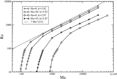
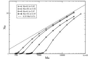
Figure 5: Reynolds and Nusselt numbers of steady two-dimensional BMC for large $Ma$ with $P=0.02$ and $L_{x}=2\pi/k$.

for the rms velocity $V$ (in thermal units) and Nusselt number $Nu$. Since the Reynolds number is $Re\sim V/P$, it becomes very difficult to resolve the small structures in the flow field for small $P$. The calculations for large $Ma$ have therefore only been done for $P=0.02$ and for selected values of $Ma$ for $P=0.01$. The results are shown in Fig. 5 for $P=0.02$. The two different domain sizes with $Ha=0$ show identical power law behavior in agreement with eq. (29), but have slightly different prefactors.

For non-zero $Ha$ there is no power-law scaling seen for $Nu$ in Fig. 5. For the rms velocity there is some indication, but with a smaller exponent than for $Ha=0$. This may, however, be misleading because the temperature field still lacks an isothermal core in the bulk, as can be seen in Fig. 2(d). The absence of power-law scaling for $Nu$ is therefore not surprising. Moreover, the estimates for the kinetic energy dissipation given in Ref. Boeck and Thess (1997) have to be corrected because of the additional Lorentz force. It is not clear if a modified scaling would emerge from an attempt to take the Lorentz force into account, which will not be made in this paper.

The Lorentz force has another interesting effect on the vorticity distribution in inertial convection. In the non-magnetic case, one finds an essentially constant vorticity inside the convection roll. The physical argument for this constant value has been given by Batchelor Batchelor (1956). Batchelor considers steady flow in a region of closed streamlines with an approximate balance of pressure gradients and advection terms in the momentum equation, i.e. high-Reynolds-number flow. In this case, convection of vorticity dominates along the streamlines, and the vorticity is therefore approximately constant along streamlines. Since the motion is assumed to be steady, viscous diffusion of vorticity across streamlines must vanish because the vorticity distribution would otherwise change with time. The vorticity therefore cannot change between neighboring streamlines, and is therefore constant in the entire region of high speed flow with closed streamlines.

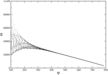
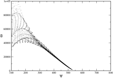
Figure 6: Vorticity-streamfunction scatter plots for steady two-dimensional BMC (in viscous units) with $Ha=10$, $Ma=32000$ (a) and $Ha=20$, $Ma=64000$ (b). The Prandtl number is $P=0.02$.

In magnetic inertial convection the additional Lorentz force is small when compared with pressure gradient and advection term, but it nevertheless dissipates energy. In a steady state there must therefore be an influx of energy into the region of closed streamlines. Since this influx must be provided by viscous diffusion, the vorticity cannot be constant as in the non-magnetic case. The scatter plots of vorticity and streamfunction shown in Fig. 6 demonstrate that this is indeed the case. The roll center is associated with the highest values of $\psi$. Viscous effects dominate near the roll boundaries where $\psi=0$, and no functional relation between $\psi$ and $\omega$ exists for small values of $\psi$. Most of this region has therefore been omitted from the scatter plots of Fig. 6 by adjusting the $\psi$ axes. For larger values of $\psi$ there is a clear functional relation between vorticity and streamfunction, and $\omega$ changes almost linearly with $\psi$. The scatter is somewhat higher for $Ha=20$, which is probably due to the lower Reynolds number caused by the stronger magnetic damping.

The approximately linear behavior of $\omega$ with $\psi$ can be understood from a modification of the derivation given by Batchelor Batchelor (1956). The starting point is the steady momentum (Navier-Stokes) equation in dimensional form,

$$\bm{v}\times\bm{\omega}=\nabla H+\nu\nabla\times\bm{\omega}-\bm{f}/\rho,$$ (30)

where the Lorentz force is denoted by $\bm{f}$ and

$$H=p/\rho+\frac{q^{2}}{2},\hskip 14.22636ptq^{2}=\bm{v}^{2}.$$ (31)

The (approximate) inviscid balance implies that

$$\bm{v}\times\bm{\omega}=\nabla H.$$ (32)

Following Batchelor (1956), one now introduces orthogonal curvilinear coordinates $(\psi,\xi)$, where the lines of constant $\xi$ are orthogonal to the streamlines with $\psi=const$. Differentials associated with $\psi$ and $\xi$ are $d\psi/q$ and $hd\xi$ in physical space, where $h(\psi,\xi)$ is unknown. The value of $H$ is constant along streamlines (Bernoulli equation), and the gradient of $H$ is therefore simply $qdH(\psi)/d\psi$. Equation (32) then takes the form

$$q\,\omega=q\,\frac{dH(\psi)}{d\psi},$$ (33)

whereby the vorticity is a function of $\psi$ only.

The next step is to integrate eq. (30) around a closed streamline. The left hand side vanishes since the line element $d\bm{l}$ is everywhere parallel to $\bm{v}$ and therefore orthogonal to $\bm{v}\times\bm{\omega}$. The first term on the right also integrates to zero, i.e. one is left with

$$\nu\oint\nabla\times\bm{\omega}\cdot d\bm{l}=\frac{1}{\rho}\oint\bm{f}\cdot d\bm{l}$$ (34)

The curl of $\omega$ is parallel to the streamline because $\omega(\psi)$, and the left hand side of eq. (34) simplifies to

$$\nu\oint\nabla\times\bm{\omega}\cdot d\bm{l}=\nu\,\frac{d\omega}{d\psi}\oint qdl.$$ (35)

When the Lorentz force is zero, this equation implies that $\omega$ is constant.

For two-dimensional convection the Lorentz force is given by

$$\bm{f}=\bm{j}\times\bm{B}=\sigma\left(\bm{v}\times\bm{B}\right)\times\bm{B}=\sigma B^{2}\left[\bm{e}_{z}\left(\bm{e}_{z}\cdot\bm{v}\right)-\bm{v}\right]=-\sigma B^{2}v_{x}\bm{e}_{x}$$ (36)

since the electric potential vanishes in this case. The integral on the right hand side of eq. (34) then becomes

$$\oint\bm{f}\cdot d\bm{l}=-\sigma B^{2}\oint v_{x}dx.$$ (37)

The integral on the right hand side of eq. (37) represents a fraction $C$ of the circulation around the streamline. One can therefore write eq. (34) as

$$\nu\,\frac{d\omega}{d\psi}\oint qdl=-\frac{\sigma B^{2}}{\rho}C\oint qdl,$$ (38)

i.e. the local slope of the vorticity-streamfunction dependence is determined by $\sigma B^{2}/\rho\nu$ and the prefactor $C$, which depends on the streamline geometry and the velocity distribution along the streamline. The almost linear decrease of $\omega$ with $\psi$ indicates that $C$ changes only weakly with $\psi$.

V Three-dimensional convection

As in the two-dimensional case, the focus of the present section is on the comparison with the non-magnetic case considered earlier Boeck and Thess (1999). The shape of the computational domain is therefore chosen in agreement with this previous work, which focused on the smallest rectangular domain compatible with a perfectly hexagonal pattern at the onset of convection. It has the aspect ratios $L_{x}=4\pi/k_{c}$, $L_{y}=4\pi/(\sqrt{3}k_{c})$ with periodic boundary conditions in the $x$- and $y$-directions. Because of the considerable computational expense of three-dimensional simulations covering a significant interval of Marangoni numbers the other parameters are fixed to $P=0$ and $Ha=10$. The corresponding wavenumber is $k_{c}=2.87$ as in the previous section. As in the non-magnetic case, the limit $P=0$ is expected to provide a consistent approximation for sufficiently small Prandtl numbers $P>0$.

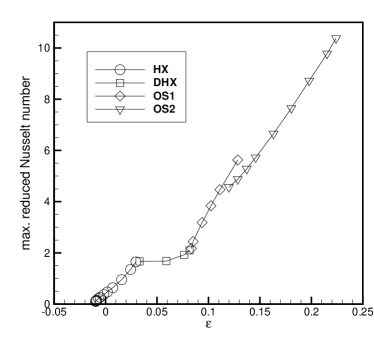
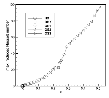
Figure 7: Solution branches for three-dimensional BMC with $P=0$ in a rectangular cell with $L_{x}=4\pi/k$,$L_{y}=4\pi/\sqrt{3}k$. Parameters are $Ha=0$, $k=1.7$ (a) and $Ha=10$, $k=2.87$ (b). The different branches are explained in the text. Values of the reduced Nusselt number $\overline{v_{z}\theta}$ correspond to maxima during the oscillation period for time-dependent convection.

The simulations were performed by systematically increasing the Marangoni number using the final state of previous runs as initial condition. Near $Ma_{c}$, the Marangoni number was also decreased to explore the subcritical range. Some simulations were started from random initial conditions to check for additional solution branches, which may be missed by the continuation approach. The main results of the simulations are summarized in the plots of Fig. 7, which show the reduced Nusselt number $\overline{v_{z}\theta}$ for different solutions as a function of the dimensionless parameter

$$\epsilon=\frac{Ma-Ma_{c}}{Ma_{c}}$$ (39)

measuring the distance from the linear instability threshold. The results for the non-magnetic case from Boeck and Thess (1999) with $Ma_{c}=57.6$ and $k_{c}=1.70$ are shown for comparison.

Two different types of stationary solutions, identified as perfect hexagons (HX) and deformed hexagons (DHX) are found in both non-magnetic and magnetic cases. These solutions are found up to $\epsilon\approx 0.24$ for $Ha=10$ whereas they only exist up to $\epsilon\approx 0.08$ for $Ha=0$. The perfect hexagons have hexagonal symmetry, which is lost in the deformed state. As in the non-magnetic case, the hexagonal convection cells are characterized by downflow in the center of the hexagons. This flow orientation is different from the hexagonal cells at $P>>1$, which have upflow in the center of the hexagon Thess and Bestehorn (1995). The hexagons exist subcritically down to $\epsilon\approx-0.008$ at $Ha=10$ and down to $\epsilon\approx-0.01$ at $Ha=0$.

Time-dependent solutions with oscillatory dynamics are marked by OS in Fig. 7. As discussed in Boeck and Thess (1999), the branch marked by OS1 corresponds to an expansion/contraction of the cells in the $x$-direction. The solution branch OS2 displays an additional periodic excitation of the mean flow component $V_{y}$ in the $y$-direction. This solution branch slightly overlaps with OS1. The OS2 branch leads to chaotic dynamics at $\epsilon\approx 0.23$, which was explored in Boeck and Vitanov (2002).

For $Ha=10$ there are three different oscillatory branches with regular dynamics. On the branch marked OS1, the hexagons oscillate in $y$-direction and in antiphase about their position as shown in Fig. 8. During the oscillation, the hexagons exchange their $y$-position relative to each other, i.e. the oscillation amplitude in the $y$ coordinate is large even at the onset. The translatory motion in $y$ is accompanied by a size oscillation of the cells. On the OS2 branch, the oscillatory motion in the $y$ direction changes its character. The hexagons do not return to their initial position but continue their motion in their respective direction. In effect, each cell performs a size oscillation and travels in either the positive or negative $y$-direction through the periodic domain. Finally, the OS3 branch is accompanied by an oscillation of the $y$ component of the mean flow. On the OS2 branch the mean flow remains zero. Chaotic dynamics appears beyond $\epsilon\approx 0.523$, i.e., $Ma\approx 413$. It is illustrated by Fig. 9, which shows as snapshot of the surface temperature perturbation, and the time series of the reduced Nusselt number.

In contrast to the non-magnetic case, no overlap could be found for the different oscillatory branches, i.e. the simulations provided a unique oscillatory solution at given Marangoni number. The onset of time dependent flow requires a higher supercriticality parameter $\epsilon$. The same applies for the excitation of the mean flow and for chaos, i.e. the magnetic field provides a considerable damping influence. Details of the transition to chaos have not been explored so far due to the considerable cost of such simulations. For $Ma\approx 400$ and larger ($\epsilon\approx 0.45$) a numerical resultion of $N_{x}=128$, $N_{y}=64$ and $N_{z}=33$ collocation points was needed in order to resolve the structures of the velocity field. The integration times were of the order $t_{\rm run}=10$ with a typical timestep $\Delta t=10^{-4}$.

VI Conclusions

The two- and three-dimensional simulations have systematically explored the influence of a vertical magnetic field on low-Prandtl-number BMC. In addition to delaying the instability, the magnetic field also extends the range of Marangoni numbers where the zero-Prandtl-number limit works for two-dimensional convection. The transition from weak to inertial convection shows some differences in comparison with the non-magnetic case of Ref.Boeck and Thess (1997), but the phenomenon itself remains unchanged. Only the asymptotic power-law scaling of inertial convection with $Ma$ could not be detected at finite Hartmann numbers, but may nonetheless be present when $Ma$ is increased further. The novel feature of inertial convection with magnetic field is the modified vorticity distribution due to the magnetic damping.

The three-dimensional simulations were restricted to $P=0$ and $Ha=10$. The appearance of time-dependent flow and chaos is again delayed by the magnetic damping, and the oscillatory solution branches differ from those found at $Ha=0$. As already done for $Ha=0$, it could be interesting to examine the chaotization in more detail.

Throughout the paper only the free-slip boundary condition at the bottom was considered. This was motivated by the observation in Ref.Boeck and Thess (1997) that the free-slip condition permits the existence of stationary rolls up to very large values of $Ma$, and thereby allows one to study this asymptotic case rather easily. No-slip conditions will lead to more complicated behavior since additional vorticity is produced at the bottom wall. However, with the additional magnetic damping the critical parameters for the free- and no-slip cases approach for large values of $Ha$, and the difference between free- and no-slip could therefore be less significant than at $Ha=0$. The free-slip condition in the present paper was chosen mainly in order to facilitate the comparison with the non-magnetic case.

The work presented here suggests at least two directions for future simulations. First, the no-slip condition and larger domain sizes should be explored in order to see if the phenomena analyzed here remain relevant in a more realistic configuration. Second, a horizontal magnetic field should lead to interesting pattern dynamics due to the imposed anisotropy. Ultimately, buoyancy and surface deformability should also be included in future numerical work.

(a)

     

(a)

(b)

(a)

(b)

(a)

(b)

(a)

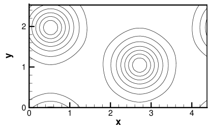
(b)

(c)

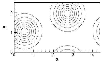
(d)

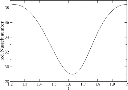
Figure 8: Time-dependent BMC with $P=0$ and $Ha=10$: surface temperature perturbation (a-c) and time evolution of $\overline{v_{z}\theta}$ (d) for oscillating hexagons at $Ma=345$. The snapshots (a-c) correspond to the beginning, middle, and end of the oscillation period shown in (d).

(a)

(b)

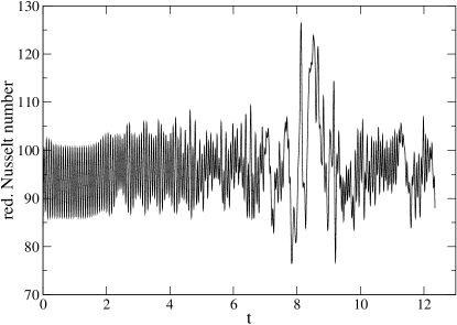
Figure 9: Chaos in BMC with $P=0$ and $Ha=10$: surface temperature perturbation (a) and time evolution of $\overline{v_{z}\theta}$ (b) at $Ma=414$. The simulation was started from the periodic solution at $Ma=410$.

Table 1: Characteristic Marangoni numbers $Ma_{i}$ and nondimensional measures $\epsilon_{i}$ for different parameter sets.

$Ha$	$k$	$Ma_{c}$	$Ma_{i}$	$\epsilon_{i}$
$0$	$2.87$	$80.0$	$115$	$0.44$
$10$	$2.87$	$271.2$	$434$	$0.60$
$0$	$3.82$	$122.7$	$187$	$0.53$
$20$	$3.82$	$757.2$	$1259$	$0.66$