Laser induced magnetization switching in films with perpendicular anisotropy: a comparison between measurements and a multi-macrospin model

Abstract

Thermally-assisted ultra-fast magnetization reversal in a DC magnetic field for magnetic multilayer thin films with perpendicular anisotropy has been investigated in the time domain using femtosecond laser heating. The experiment is set-up as an optically pumped stroboscopic Time Resolved Magneto-Optical Kerr Effect magnetometer. It is observed that a modest laser fluence of about 0.3 mJ/cm² induces switching of the magnetization in an applied field much less than the DC coercivity (0.8 T) on the sub-nanosecond time-scale. This switching was thermally-assisted by the energy from the femtosecond pump-pulse. The experimental results are compared with a model based on the Landau Lifschitz Bloch equation. The comparison supports a description of the reversal process as an ultra-fast demagnetization and partial recovery followed by slower thermally activated switching due to the spin system remaining at an elevated temperature after the heating pulse.

I Introduction

There is currently considerable interest in ultra-fast laser-induced magnetization processes. Since the demonstration by Beaurepaire et al. beaurepairePRL96 that the magnetization can respond on the picosecond timescale to heat pulses produced by femtosecond lasers, a number of groups kimelNATURE04 ; kimelNATURE05 ; hohlfeldPRB01 have studied magnetization processes on this timescale. Experiments generally use pump-probe processes in which a high energy laser pulse is used to heat the sample and a low energy probe pulse (split from the main pulse) is used to monitor the magnetic response using the Magneto-Optical Kerr Effect (MOKE). Much of this work has investigated the dynamics of the destruction and recovery of the magnetization, which can occur on the sub-picosecond timescale, although the recovery can take an order of magnitude longer due to frustration effects among large numbers of nucleation sites at which the recovery starts locally kazantsevaEPL08 .

The dynamics of reversal during a pulsed laser experiment in the presence of an applied field has received less attention. Hohlfeld et al. hohlfeldPRB01 investigated the magnetization reversal induced by 100 fs laser pulses in a GdFeCo Magneto-Optical recording medium with perpendicular anisotropy. They observed an ultra-fast demagnetization of the film occurring within the first picosecond; followed by a slower recovery, taking nearly a nanosecond, in the direction of the applied field as the heat drains from the media layer. They analyzed their measurements using the Bloch equation and concluded that the reversal process was governed by the nucleation and growth of domains in the applied field.

Laser assisted magnetization processes have considerable potential for future ultra-high density recording systems. Essentially, the path to higher densities requires continuous reduction in the grain volume $V$ of the storage medium, necessitating an increase in the magneto-crystalline anisotropy energy density $K$ in order to preserve a sufficiently large value of the parameter $KV/{k_{\mathrm{B}}}T$ ($\sim 60$) to ensure thermal stability of written information weller . However, the large value of $K$ impacts the writability of the information, and some scheme is required to overcome this problem. A promising solution is Hybrid or Heat Assisted Magnetic Recording (HAMR) rottmayer in which the medium is heated in order to lower the anisotropy and thereby allow information to be written to the medium. Since this is a relatively new field the magnetization reversal mechanisms are not well understood. Although the work of Hohlfeld et al. hohlfeldPRB01 has demonstrated thermally activated domain processes in magneto-optical media, perpendicular recording requires relatively weakly coupled granular media in which domain processes are not the dominant reversal mechanism.

This paper presents time-domain measurements of the magnetization reversal process induced by an ultra-fast laser pulse in a thin film with perpendicular anisotropy. The film was especially designed to have a low Curie temperature in order to simplify the experiments. We compare the results with a computational model using the Landau-Lifshitz-Bloch (LLB) equation garaninPRB97 , which is ideally suited to simulation of magnetization processes up to and beyond ${T_{\mathrm{c}}}$ and has been shown chubykaloPRB06 ; atxitiaAPL07 to give an excellent description of the physics of pulsed laser processes. It is concluded that the magnetization response consists of a fast demagnetization followed by a slower response in which the magnetization evolves into the field direction by a process of thermally activated transitions over the local energy barriers. Our LLB-micromagnetic model is shown to give a good description of the physics of the reversal process on both timescales.

II Method

The experiment is a stroboscopic pump-probe experiment using a strong laser pulse to initiate a change in the magnetic state of the sample and a weak probe pulse to observe the resulting magnetization dynamics via the MOKE. The sample is mounted in a spin-stand which first moves the magnetic film through a reset field of magnitude $\sim 1$T for a duration of $0.2$ ms which ensures that the sample is in a remanent state before exposure to each laser pulse. Fig. 1 illustrates the spin-stand arrangement, with the insert showing the temporal field profile experienced by the magnetic film. After resetting to saturation the sample then moves into a perpendicular applied field from an electromagnet (field range of $\pm$0.52 T). We note that the field applied is always lower than the static coercivity of the sample as measured at room temperature by a vibrating sample magnetometer. At the center of the pole piece a small hole allows optical access to the sample at which point the sample is exposed to the pump-pulse. The laser pulses arrive at a rate of 1 kHz but the rotation of the spin-stand (about 7,000 rpm) ensures that freshly saturated film arrives between pulses.

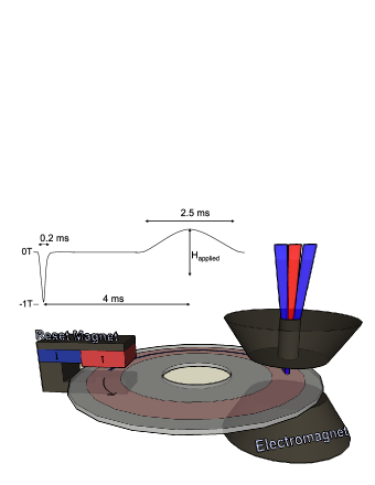
Figure 1: Illustration of spin-stand arrangement used to ensure the materials magnetization is reset between pump pulses.

The stroboscopic experiment uses a Libra laser system (made by Coherent) which can produce a 1 kHz stream of 1 mJ, 150 fs pulses of 800 nm radiation. This beam is attenuated, the probe beam is split off and frequency doubled to 400 nm. The pump beam is routed around an optical delay line with 17 fs resolution over a 1 ns range and then focused at normal incidence to a spot approximately 800 $\mu$m in diameter on the disk surface. The probe beam is polarized and then brought to a 400 $\mu$m focal spot, centered on the pump beam with a power level of about 1/20th of the pump. Because the probe is only half the diameter of the pump it must be noted that there will be a temperature distribution across the region probed. The probe approaches the sample surface at near normal incidence; this polar MOKE geometry yields sensitivity to the out-of-plane component of magnetization. The reflected probe beam is directed into an optical bridge detector which uses a Wollaston prism to split the beam into two orthogonal polarized components which impinge on a two segment photo-detector. By rotating the detector to the angle where the output of the two polarization channels (A & B) are approximately equal, then the difference between them (A-B) is sensitive to small changes of the polarization angle of the reflected probe which in turn is proportional to $m_{z}$. The sum (A+B) is sensitive to changes in reflectivity $\Delta R$, which is associated with temperature changes and stress waves due to processes such as lattice expansions. In order to improve immunity to laser drift the pump beam was chopped and lock-in amplifiers used to detect the sum and difference signals. This makes the measurement sensitive to the difference between the state of the sample without the pump pulse applied and the state induced by the pump-pulse. Therefore the measurements are relative and it is difficult to assign an absolute scale to the magnetization changes.

III Experimental Results

For characterization of the sample the quasi-static hysteresis loop was measured. Of particular importance is the coercivity, which on this timescale is $\sim$ 0.85T, and the saturation magnetization ${M_{\mathrm{s}}}$, which is equal to 0.35 $\times 10^{6}$ A/m. The coercivity of course is already greater than the field applied during our pulsed field experiment. However, it is important to note that the dynamic coercivity on the timescale of the pulsed laser experiment is even larger. The intrinsic coercivity ($H_{0}$) and the thermal stability factor ($KV/{k_{\mathrm{B}}}T$) were measured by making a series of time dependent coercivity measurements and fitting to Sharrock’s law sharrock . The intrinsic coercivity is related to the anisotropy field and is expected to give a reasonable estimate of the coercivity at the nanosecond timescale. The value of $H_{0}$ was found to be 1.4T; a factor of almost 3 greater than the maximum field available from the electromagnet. Separate measurements determined the anisotropy $K$ to be $4\times 10^{6}$ J/m³, from which a grain size of 10nm was estimated.

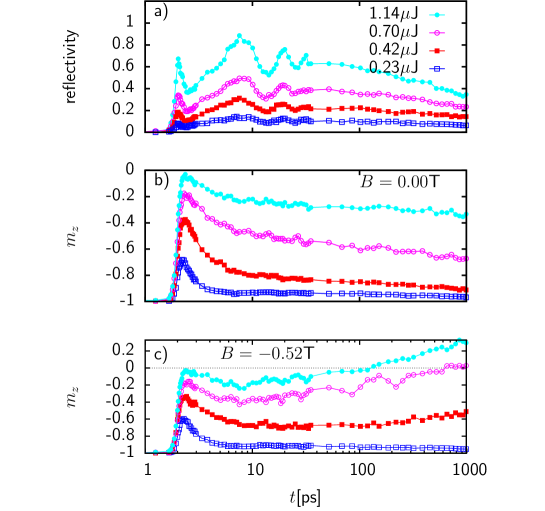
Figure 2: Series of measurements in an applied reversing field of 0.52T for different laser pulse energies. a) shows the reflectivity data, b) the $m_{z}$ component of magnetization, and c) shows the response in the presence of a reversing field

Fig. 2 shows a set of time-resolved measurements on the sample. Fig. 2 (a) shows the reflectivity data, Fig. 2 (b) shows the dynamic magnetic response for zero applied field and Fig. 2 (c) shows the response in the presence of a reversing field of 0.52 T. The laser pulse energy is varied up to 1.14 $\mu$J per pulse (which corresponds to a fluence of approximately 0.23 mJ/cm²). This value is the largest than can safely be applied to this sample as energy fluences above about 0.5 mJ/cm² damage the sample. The sample reflectivity data shown in Fig. 2 (a) is a probe of the electron/lattice temperature in the system. It indicates that the same temperature profile is generated each time and that the temperature scales linearly with pulse energy. The reflectivity measurement has three distinct features. Within the first 5 ps is a large peak having a width of 350 fs, which corresponds to the large rise in electron temperature caused by the arrival of the 150 fs laser pulse. The electron system then establishes thermal equilibrium with the lattice which creates the second, rather broader, peak 20 ps later. In reality the peak temperature the lattice reaches is much lower than that for the electrons; however, it seems that in this sample the change in reflectivity is more sensitive to the lattice temperature than the electron temperature. The waves seen superimposed onto the lattice temperature peak during the 3-35 ps time frame are probably stress pulses launched into the film by the laser heating of the surface, which reflect off the interface with the glass substrate. The time between peaks is 12 ps, which, given the film and interlayer thickness of 25 nm, suggests a propagation speed of 4,100 m/s; consistent with the speed of sound in a typical metal. The sample appears to cool rather slowly as the lattice temperature has only fallen to half its peak value after 1 ns. This reflects the fact that in this film there is no heat sink to absorb the heat. Fig. 2 (b) and (c) show the magnetization dynamics in applied fields of 0 and -0.52 T respectively. Fig. 2 (c) clearly demonstrates heat assisted reversal due to the pulse. For pulse energies above $\sim 0.5\mu$J the sample is seen to cool with the magnetization aligning along the applied field. Recalling that the dynamic coercivity estimated from magnetic measurements is around 1.46T, this demonstrates a significant heat-assistance during the sub-nanosecond reversal process.

We now consider in detail the processes involved in the magnetization dynamics, which involves three characteristic timescales as illustrated in Fig. 2. The initial phase involves a rapid demagnetization of the sample lagging the change in reflectivity by only 50 fs. The demagnetization takes about 500 fs, independent of the applied field. This is consistent with the normal expectation of a rapid demagnetization as previously demonstrated experimentally beaurepairePRL96 ; kimelNATURE05 ; hohlfeldPRB01 and theoretically koopmansJMMM05 ; kazantsevaEPL08 . The sample then appears to partially recover its magnetization in the original direction, on a timescale independent of the applied field. It is interesting to note that the rate of recovery from the demagnetization peak is related to the amount of demagnetization achieved - a pattern consistent with the calculations of Kazantseva et al. kazantsevaEPL08 . Throughout the whole process the only apparent field dependence occurs in the longer time-scale dynamics (20ps-1ns). Over this timescale, for the higher laser powers, a gradual reversal of the magnetization is seen.

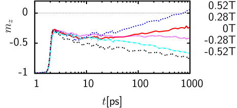
Figure 3: Series of measurements of the temporal variation of $m_{z}$ in various applied reversing fields for a constant laser pulse energy.

A similar systematic trend is also exhibited by the temporal variation of $m_{z}$ at constant laser power in various applied fields, as shown in Fig. 3. The initial disappearance and recovery of the magnetization is similar for all applied fields, but with increasing positive field the long-term trend is clearly toward positive magnetization.

The form of the dynamics, involving a trend against the field direction followed by a slow reversal into the field direction is apparently somewhat counter-intuitive. However, the form of the magnetization evolution can be explained by consideration of the different timescales associated with processes at the atomic and macrospin length scales. Within each grain or ’macrospin’ the disappearance and recovery of the magnetization will be governed by the longitudinal relaxation time, which is temperature dependent but typically of a sub-picosecond timescale, which is consistent with the experimental data of Fig. 2 (b) and (c). However, after this process the system remains at an elevated temperature for around 1ns, so there is a possibility of thermally activated magnetization reversal. This will have a characteristic timescale determined by the macrospin energy barrier, which is lowered by the reduction of the anisotropy constant at elevated temperature, but typically has values much greater than 1ps. On this basis we would expect to see a fast reduction and recovery of the magnetization due to atomic processes on the picosecond timescale with a slower relaxation into the field direction due to thermally activated reversal of the macrospins. In order to test this hypothesis in relation to the experimental results we have developed a computational model of the laser heating process based on the LLB equation which has been shown atxitiaAPL07 to give a good description of magnetization processes over both characteristic timescales.

IV Dynamic model of laser heating process

We have developed a computational model of laser-induced magnetization dynamics of a thin film with perpendicular anisotropy. Consistent with experiments we assume a granular microstructure for the film. For simplicity we assume, in these initial calculations, a mono-disperse grain size and anisotropy. Inter-granular magneto-static interactions are included, but the grains are taken as exchange decoupled. As mentioned previously the Landau-Lifschitz Gilbert (LLG) equation cannot be used for models of laser heating since it does not allow longitudinal fluctuations of the magnetizationkoch ; slav . In the following, we use the LLB equation garaninPRB97 for the thermodynamic simulation of the laser-induced magnetization switching. As described in detail in Ref. kazantsevaPRB08 ; atxitiaAPL07 , the LLB equation has been shown by comparison with atomistic calculations to give a remarkably good description of the physics of ultra-fast high temperature dynamics. The LLB equation can be written as

$$\mathbf{\dot{m}}_{i}=-\tilde{\gamma}[\mathbf{m}_{i}\times\mathbf{H}^{i}_{\mathrm{eff}}]+\frac{\tilde{\gamma}\alpha_{||}}{m_{i}^{2}}\left(\mathbf{m}_{i}\cdot(\mathbf{H}^{i}_{\mathrm{eff}}+\boldsymbol{\zeta}^{i}_{||})\right)\mathbf{m}_{i}$$

$$\qquad{}-\frac{\tilde{\gamma}\alpha_{\perp}}{m_{i}^{2}}\left[\mathbf{m}_{i}\times\left[\mathbf{m}_{i}\times\left(\mathbf{H}^{i}_{\mathrm{eff}}+\boldsymbol{\zeta}^{i}_{\perp}\right)\right]\right].$$ (1)

Note, that besides the usual precession and relaxation terms in the LLG equation (see Ref. nowakBOOK07 for more details), the LLB equation contains an additional term which controls the longitudinal relaxation. Here, ${\bf m}_{i}$ is a spin polarization which is not assumed to be of constant length and even its equilibrium value $m_{\rm e}(T)$ is temperature dependent. ${\alpha_{\parallel}}$ and $\alpha_{\perp}$ are dimensionless longitudinal and transverse damping parameters.

The LLB equation is valid for finite temperatures and even above ${T_{\mathrm{c}}}$ though the damping parameters and effective fields are different below and above ${T_{\mathrm{c}}}$. For $T\leq{T_{\mathrm{c}}}$ the damping parameters are

$${\alpha_{\parallel}}=\lambda\frac{2T}{3{T_{\mathrm{c}}}}\quad\alpha_{\perp}=\lambda(1-\frac{T}{3{T_{\mathrm{c}}}})$$ (2)

and for $T\geq{T_{\mathrm{c}}}$ the damping parameters are equal,

$$\alpha_{\perp}=\alpha_{\parallel}=\frac{2\lambda T}{3{T_{\mathrm{c}}}}.$$ (3)

In these equations $\lambda$ is a microscopic parameter which characterizes the coupling of the individual, atomistic spins with the heat bath.

Thermal fluctuations garaninPRB04 are included as an additional noise term ${\boldsymbol{\zeta}}^{i}_{l}(t)$ with $l=\perp,\parallel$, $\langle{\boldsymbol{\zeta}}^{i}_{l}(t)\rangle=0$ and

$$\langle{\zeta}_{l}^{i,\nu}(0){\zeta}_{l}^{j,\eta}(t)\rangle={2k_{B}T\over\tilde{\gamma}\alpha_{l}M_{\mathrm{s}}^{0}\Delta^{3}}\delta_{\nu\eta}\delta_{ij}\delta(t),$$ (4)

where $i,j$ denotes lattice sites and $\nu,\eta$ the Cartesian components. Here, $\Delta^{3}$ is the volume of the grains and $M_{\mathrm{s}}^{0}$ is the value of the spontaneous magnetization at zero temperature.

The effective fields are $\mathbf{H}_{\mathrm{eff}}^{i}=-\frac{1}{M_{\mathrm{s}}^{0}}\frac{\delta f}{\delta\bf{m}_{i}}$, with $f$ the free energy density. The total local field is given by garaninPRB97

$$\mathbf{H}_{\mathrm{eff}}^{i}=\mathbf{H}+\mathbf{H}_{A}^{i}+\mathbf{H}_{\rm dipol}^{i}+\left\{\begin{array}[]{cc}\;\;\;\;\;\;\;\;\frac{1}{2\tilde{\chi}_{\|}}\left(1-\frac{m^{2}_{i}}{m_{\rm e}^{2}}\right)\mathbf{m}_{i}&T\leq{T_{\mathrm{c}}}\\ -\frac{1}{\tilde{\chi}_{\|}}\left(1+\frac{3{T_{\mathrm{c}}}m^{2}_{i}}{5(T-{T_{\mathrm{c}}})}\right)\mathbf{m}_{i}&T\geq T_{\mathrm{c}}\end{array}\right.\mathbf{.}$$ (5)

with the anisotropy field

$$\mathbf{H}_{A}^{i}=-\frac{\left(m_{x}^{i}\mathbf{e}_{x}+m_{y}^{i}\mathbf{e}_{y}\right)}{\tilde{\chi}_{\perp}}$$ (6)

which makes the $z$ axis the easy axis of the model, and the dipolar field

$$\mathbf{H}_{\rm dipol}^{i}=\frac{M_{\mathrm{s}}^{0}\Delta^{3}\mu_{0}}{4\pi}\sum\limits_{i<j}\textstyle\frac{{3({\bf m}_{i}\cdot{\bf e}_{ij})({\bf e}_{ij}\cdot{\bf m}_{j})-\bf m}_{i}\cdot{\bf m}_{j}}{r_{ij}^{3}}$$ (7)

Note, that the susceptibilities $\tilde{\chi}_{l}$ are defined by $\tilde{\chi}_{l}=\partial m_{l}/\partial H_{l}$. At lower temperatures the perpendicular susceptibility $\tilde{\chi}_{\perp}$ is related to the anisotropy $K$ via $\tilde{\chi}_{\perp}=M_{\mathrm{s}}^{0}m_{\rm e}^{2}/(2K)$. garaninPRB97 . One problem for the application of the LLB equation is that one has to know the functions for the spontaneous equilibrium magnetization $m_{\rm e}(T)$, the perpendicular ($\tilde{\chi}_{\perp}(T)$) and parallel ($\tilde{\chi}_{\parallel}(T)$) susceptibilities. Here, we use the functions for FePt gained from a Langevin dynamics simulation of an atomistic spin model as described in kazantsevaPRB08 . In the following, we assume that these functions reflect the correct temperature behavior. We normalize the perpendicular susceptibility such that its value at 300K is consistent with experimentally determined values for CoPt ($K=3.94\cdot 10^{5}$ J/m³) determined by the rotation method Lu . The input functions are shown in Fig. 4.

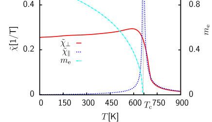
Figure 4: Spontaneous equilibrium magnetization and parallel and transverse susceptibility vs. temperature.

The LLB equation is solved numerically by using Langevin dynamics simulations as described in nowakBOOK07 . For our simulations we chose a disc of $32\times 32\times 1$ cells, with a grain size $\Delta$ of 10nm.

V Comparison between Multi-Macro Spin Model and Experiment

In order to make a comparison with the experimental data it is necessary to have an approximation to the temporal variation of the temperature pulse caused by the heating. Because of the complex behavior of the reflectivity as discussed by Djordjevic et al. djordjevic it is not feasible to use this property to determine the temperature profile in this work. Instead we make the simplifying assumption that, at low laser powers, the magnetization closely follows the electron temperature during the heating and initial recovery phase; an assumption essentially borne out by calculations in Ref. kazantsevaEPL08 using an atomistic model, where fast demagnetization and recovery were found for low peak electron temperatures. Following Ref. kazantsevaEPL08 , we assume that the photon energy is transfered to electrons and that the magnetization is directly coupled to the electron temperature $T_{\mathrm{e}}$ within a two-temperature model zhangBOOK02 , expressed as the following coupled differential equations for the electron and phonon temperatures, $T_{\mathrm{e}},T_{\mathrm{l}}$ respectively:

$$C_{\mathrm{e}}{{\mathrm{d}}T_{\mathrm{e}}\over{\mathrm{d}}t} = -G_{\mathrm{e}l}(T_{\mathrm{e}}-T_{\mathrm{l}})+P(t)$$

$$C_{\mathrm{l}}{{\mathrm{d}}T_{\mathrm{l}}\over{\mathrm{d}}t} = G_{\mathrm{e}l}(T_{\mathrm{e}}-T_{\mathrm{l}}),$$ (8)

where $C_{\mathrm{e}},C_{\mathrm{l}}$ are electron and lattice specific heat constant, $G_{\mathrm{e}l}$ is a coupling constant and $P(t)$ is the laser fluence. Eqs. 8 can easily be solved numerically to generate the time variation of $T_{\mathrm{e}},T_{\mathrm{l}}$. We determine the parameters of the two-temperature model by fitting to the form of the initial magnetization decay and recovery, assuming a Gaussian laser profile.

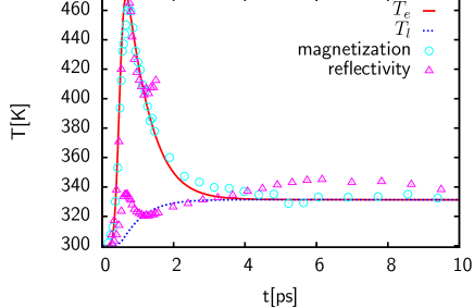
Figure 5: Graph showing the electron temperature ($T_{\mathrm{e}}$) and the lattice temperature ($T_{\mathrm{l}}$) simulated by the two-temperature model. Scaled reflectivity and magnetization data are also included for comparison.

Fig. 5 shows a comparison of the two-temperature model with the data from the reflectivity and low laser power magnetization measurements in order to estimate physically reasonable parameters for the model. The time-scale of the peak in electron temperature $T_{\mathrm{e}}$ matches the demagnetization peak in the magnetization data and the initial peak in the reflectivity data. The lattice temperature $T_{\mathrm{l}}$ reaches its peak value on the same time-scale as the second rise in the reflectivity data. For use in the computational model an interpolation function was fitted to the $T_{\mathrm{e}}$ predicted above. Different laser fluences were simulated by scaling the results to the peak electron temperature ($T_{\rm e}^{\rm p}$), which becomes a main parameter in the comparison with experiment.

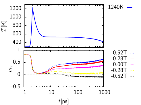
Figure 6: Calculated time dependence of the $z$-component of the magnetization for different applied magnetic fields. $\frac{KV}{{k_{\mathrm{B}}}T}=76$ with K = $3.2\cdot 10^{5}$ J/m³ and $V$ = (10 nm)³ at room temperature. ($T_{\rm e}^{\rm p}$ = 1240K, $\lambda=0.1$)

We first describe calculations with the assumption of a spatially uniform temperature profile. The model parameters used correspond to a material with a ${T_{\mathrm{c}}}$ of 660K, ${M_{\mathrm{s}}}$ = 1.75 $\times 10^{5}$ A/m, an out-of-plane anisotropy $K$ = 3.2 $\times 10^{5}$ J/m³ and a damping constant $\lambda$ of 0.1. The material is broken up into $32\times 32$ cells of size 10 nm which are exchange decoupled in order to model the granular structure of a recording medium. The intention is to outline the effects of the major parameters in the model, namely the applied field, peak electron temperature and the coupling parameter. Fig. 6 shows the temporal response of the magnetization to a laser pulse giving rise to a peak electron temperature of $1240K$ assuming a coupling parameter of $\lambda=0.1$. It can be seen that the simulation gives a reasonable qualitative description of the time evolution of the magnetization following a laser pulse. Specifically we note the initial fast demagnetization and recovery. In the case of a positive field the magnetization recovers to the equilibrium value in the positive sense. In a reversing field the initial recovery is followed by a slow reversal of the magnetization toward the field direction which, in the model, can be unambiguously attributed to thermally activated transitions over the particle energy barriers, supporting the earlier interpretation of the experimental data.

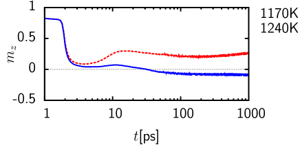
Figure 7: Calculated time dependence of the $z$-component of the magnetization for two different peak temperatures. $\frac{KV}{{k_{\mathrm{B}}}T}=76$ with K = $3.2\cdot 10^{5}$ J/m³ and $V$ = (10 nm)³ at room temperature. ($\lambda=0.1$,$B_{z}=-0.52$T)

Fig. 7 explores the effect of increasing the peak electron temperature. As might be expected, the effect of this parameter is to lead to a more complete demagnetization during the laser pulse. After the high temperature pulse the system remains demagnetized due to the high temperature remaining after the pulse.

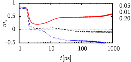
Figure 8: Calculated time dependence of the $z$-component of the magnetization for different values of $\lambda$. $\frac{KV}{{k_{\mathrm{B}}}T}=76$ with K = $3.2\cdot 10^{5}$ J/m³ and $V$ = (10 nm)³ at room temperature ($T_{\rm e}^{\rm{p}}$ = 1240 K, $B_{z}=-0.52$T)

Finally, we consider the effect of the coupling parameter $\lambda$. Calculations for 3 different values of $\lambda$ are shown in Fig. 8. Here, it can be seen that the effect of increasing $\lambda$ is to achieve a more rapid demagnetization. This is consistent with previous calculations kazantsevaEPL08 , where the effect is interpreted in terms of the more efficient transfer of energy into the spin system at large $\lambda$ leading to a more complete demagnetization for a given laser pulse width. Clearly the increased demagnetization caused by the stronger coupling to the conduction electron system results in an increased heat assistance of the magnetization reversal.

In addition to the material parameters, the peak electron temperature and the coupling constant are seen to be important in the heat assisted reversal process. Although the model reproduces the essential physics of the reversal process, particularly the different behavior on the timescales of longitudinal relaxation (fast demagnetization) and transverse relaxation (super-paramagnetic fluctuations) qualitative agreement only is obtained with experimental data. Specifically, the value of $KV/{k_{\mathrm{B}}}T=76$ (at room temperature) used in the simulations is rather small in comparison with the experimentally determined values. In order to obtain closed agreement with experiment it is necessary to include an important experimental factor; specifically the fact that the probe pulse area is comparable to that of the pump. This introduces a significant temperature gradient within the probe area, which must be taken into account in the calculations.

Here, we model this effect using a Gaussian temperature profile for the laser spot. The diameter of the spot used in the model calculations is much smaller than in the experiments ($800\mu m$). This would be an unrealistic approximation if the magnetization reversal involved domain wall processes; however, since the grains are essentially decoupled in the experimental films this simplified model is able to gives some insight into the effects of the temperature profile. Since both pump and probe beams have a Gaussian temperature variation, we take the temperature variation to be of the form $T(r)\propto\exp(-r^{2}/r^{2}_{\mathrm{pump}})$, with $r_{\mathrm{pump}}$ the radius of the pump beam. The MOKE signal is assumed to be proportional to the product of the magnetization with a sensitivity function. The sensitivity function is proportional to the area of material generating the MOKE signal at a particular radius and the light intensity at that radius, which has a Gaussian weighting, i.e. $\propto m_{z}r\exp(-r^{2}/r^{2}_{\mathrm{probe}})dr$, with $r_{\mathrm{probe}}$ the radius of the probe. A numerical integration over the probe area was carried out to determine the calculated MOKE signal from the film.

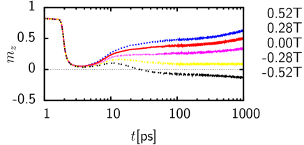
Figure 9: $z$-component vs. time for different applied magnetic fields $B_{z}$. $\frac{KV}{{k_{\mathrm{B}}}T}=95$ with K = $3.94\cdot 10^{5}$ J/m³ and $V$ = (10 nm)³ at room temperature ($T_{\rm e}^{\rm{p}}$ = 1480K, $\lambda=0.1$)

The introduction of a temperature profile results in a qualitative agreement with experiment using parameters close to the measured values. Fig. 9 shows calculations of the time dependence of the magnetization following a laser pulse with a peak temperature of $1480$K for different values of the applied magnetic field. The parameters used were $M_{\mathrm{s}}^{0}=0.4\times 10^{6}$ A/m, giving a room temperature value close to the measured (VSM) values of $0.32\times 10^{6}$ A/m. The anisotropy constant $K^{0}$ at zero temperature was taken as $3.94\times 10^{5}$J/m³, which gives a value of $KV/{k_{\mathrm{B}}}T=95$ at room temperature, in good agreement with the experimentally determined value of 96. It is interesting to note that if a larger value of $M_{\mathrm{s}}^{0}$ is used then system appears to lock into a domain-state during reversal, which suggests that even at elevated temperatures the inter-granular magneto-static interactions can play an important role. The exchange coupling can be added, but values as big as 10% do not change the results significantly. As noted by Kazantseva et al. kazantsevaEPL08 , changes in the value of the damping constant affect the amount of energy the magnetic system absorbs from the initial heat pulse and so how much of a demagnetization is achieved for a given peak electron temperature. In addition there is a slight broadening in the demagnetization peak.

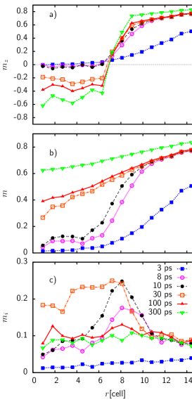
Figure 10: Radial magnetization in a 0.52T field as a function of time after the laser pulse. (a) shows the perpendicular component $m_{z}$, (b) the magnitude $m$, and (c) the magnitude of the in-plane component $m_{i}$

Fig. 10 shows a more detailed analysis of the LLB simulations, indicating that the magnetization dynamics are an ultra-fast demagnetization and recovery caused by the electron temperature peak, after which the elevated temperature of the lattice causes a gradual switching of the individual grains of material. Fig. 10 shows the temporal evolution of the radial magnetization defined such that $m_{\alpha}(r)dr$ is the spatially averaged magnetization over the annulus $r\rightarrow r+dr$; here $\alpha$ is the z-component of the magnetization $m_{z}$ (Fig. 10(a)), the total magnetization (Fig. 10(b)), and the in-plane magnetization, defined as the spatial average of $(m_{x}^{2}+m_{y}^{2})^{1/2}$ (Fig. 10(c)).

We consider the behavior of two distinct regions; the central region for radius $<$ 7 cell radii, where the temperature exceeds ${T_{\mathrm{c}}}$ during the pulse leading to complete demagnetization, and the outer region which doesn’t exceed ${T_{\mathrm{c}}}$. The variation of the total magnetization (Fig. 10(b)) is consistent with previous calculations kazantsevaEPL08 . Specifically, the rate of recovery of the magnetization depends upon the magnetic state. Within the central region the material is completely disordered and the recovery of the magnetization is relatively slow due to the need for the magnetization to recover from highly disordered states. In the outer region the magnetization retains some memory of the initial state, which results in a rapid recovery kazantsevaEPL08 .

Of most importance in terms of heat assisted reversal is the behavior of the central region. Heat assistance of the reversal is demonstrated clearly in Fig. 10(a), which shows reversal of the central (heated) region while the magnetization in the outer region is not switched. The nature of the reversal in the central region is further investigated using the radially resolved in-plane component of the magnetization, which is shown in Fig. 10(c). It is interesting to note that a large in-plane component develops on the timescale of $10\rightarrow 30$ ps. This results from the relatively random recovery of the direction of the magnetization after cooling though ${T_{\mathrm{c}}}$. This contributes to the magnetization reversal in two ways. Firstly, some of the grains take on a negative sense of the magnetization on recovery. Others will recover in a positive sense but at an angle greater than the energy maximum as the anisotropy increases; these grains are most likely to switch into the negative direction as the temperature decreases. At longer timescale, and consequently lower temperatures, the in-plane component reduces as the magnetization of each grain begins to lie preferentially along the easy anisotropy axis. However, the in-plane component does not completely disappear, probably reflecting the Boltzmann distribution of the magnetization direction within each grain. In addition to these mechanisms it is also likely that there will be thermally activated reversal over the energy barriers at the elevated temperatures. Along with the increase in spontaneous magnetization as the film cools this would contribute to the gradual increase in $m_{z}$ over timescales of 1 ns.

VI Conclusions

We have presented laser pump-probe measurements which show a clear heat assistance from the laser pulse for switching the magnetization state. This is demonstrated by the ability to switch in an externally applied field with a magnitude lower than the intrinsic coercivity. The experiments show a rapid demagnetization and recovery followed by a slow evolution of the magnetization into the field direction. This is consistent with the existence of two characteristic relaxation times; the longitudinal and transverse relaxation times. The former is atomic-scale processes and is typically of the sub-picosecond order, whereas the transverse relaxation time reflects transitions over the energy barrier and can be orders of magnitude longer. In order to investigate the reversal mechanism we have developed a micromagnetic model based on the LLB equation which naturally includes both timescales. The LLB model calculations are in good quantitative agreement with the experimental data, as long as the the temperature gradient across the probe pulse is included. It appears that on the short time-scale (2 ps) there is a rapid demagnetization of $m_{z}$ due to an associated loss of ${M_{\mathrm{s}}}$ via the longitudinal relaxation. There is a partial recovery of $m_{z}$ in the original direction as ${M_{\mathrm{s}}}$ starts to recover. However, the switching is assisted by the recovery of the magnetization of individual grains in random directions as the system cools through ${T_{\mathrm{c}}}$. On the longer time-scale the reversal of $m_{z}$ in the applied field may also be assisted by thermally activated switching caused by the elevated lattice temperature. The elevated temperature has the effect of lowering the anisotropy energy barriers (due to the reduced values of the Magnetocrystalline anisotropy energy) and also provides the thermal energy to induce the transitions. The complex behaviour requires a model including both the longitudinal and transverse relaxation times, which is included here using the LLB equation. Our LLB based calculations encapsulate the physics of the heat-assisted reversal process and suggest the LLB equation as a physically realistic model for Heat Assisted Magnetic Recording.

VII Acknowledgments

The authors would like to acknowledge the CLF (Central Laser Facility) who loaned the laser system used in the project and Dr. S. Lepadatu for his assistance in developing the experiment.

References

- (1) E. Beaurepaire, J.-C. Merle, A. Daunois, and J. Y. Bigot, Phys. Rev. Lett. 76, 4250 (1996).
- (2) J. Hohlfeld, T. Gerrits, M. Bilderbeek, T. Rasing, H. Awano, and N. Ohta, Phys. Rev. B 65, 012413 (2001).
- (3) A. V. Kimel, A. Kirilyuk, A. Tsvetkov, R. V. Pisarev, and T. Rasing, Nature 429, 850 (2004).
- (4) A. V. Kimel, A. Kirilyuk, P. A. Usachev, R. V. Pisarev, A. M. Balbashov, and T. Rasing, Nature 435, 655 (2005).
- (5) N. Kazantseva, U. Nowak, R. W. Chantrell, J. Hohlfeld, and A. Rebei, Europhys. Lett. 81, 27004 (2008).
- (6) D Weller and A Moser, IEEE Trans. Mag., 35, 4423 (1994)
- (7) R.E Rottmayer et.al., IEEE Trans. Mag., 42, 2417 (2006)
- (8) G. Grinstein and R. H. Koch, Phys. Rev. Lett. 90, 207201 (2003).
- (9) V.V. Dobrovitski, M. I. Katsnelson and B. N. Harmon, Phys. Rev.Lett. 90, 067201 (2003).
- (10) D. A. Garanin, Phys. Rev. B 55, 3050 (1997).
- (11) O. Chubykalo-Fesenko, U. Nowak, R. W. Chantrell, and D. Garanin, Phys. Rev. B 74, 094436 (2006).
- (12) U. Atxitia, O. Chubykalo-Fesenko, N. Kazantseva, D. Hinzke, U. Nowak, and R. W. Chantrell, Appl. Phys. Lett. 91, 232507 (2007).
- (13) M. P. Sharrock, J. Appl. Phys. 76, 6413 (1994)
- (14) B. Koopmans, H. H. J. E. Kicken, M. van Kampen, and W. J. M. de Jonge, J. Magn. Magn. Mat. 286, 271 (2005).
- (15) N. Kazantseva, D. Hinzke, U. Nowak, R. W. Chantrell, U. Atxitia, and O. Chubykalo-Fesenko, Phys. Rev. B 77, 184428 (2008).
- (16) V.W. Guo, Bin Lu, X.W Wu, G Ju, B Valcu and D Weller, J Appl. Phys., 99, 08E918 (2006)
- (17) U. Nowak, in Handbook of Magnetism and Advanced Magnetic Materials, Vol. 2, Micromagnetism, edited by H. Kronmüller and S. Parkin (John Wiley & Sons Ltd., Chichester, 2007).
- (18) D. A. Garanin and O. Chubykalo-Fesenko, Phys. Rev. B 70, 212409 (2004).
- (19) M. Djordjevic, M. Lüttich, P. Moschkau, P. Guderian, T. Kampfrath, R. G. Ulbrich, M. Mnzenberg, W. Felsch, J. S. Moodera, Phys. Stat. Sol. (c) 3, 1347 1358 (2006)
- (20) G. Zhang, W. Hübner, E. Beaurepaire, and J.-Y. Bigot, in Spin Dynamics in Confined Magnetic Structures I, edited by B. Hillebrands and K. Ounadjela (Springer-Verlag, Berlin Heidelberg New York, 2002), p. 245.