Longest convex chains

Abstract.

Assume $X_{n}$ is a random sample of $n$ uniform, independent points from a triangle $T$. The longest convex chain, $Y$, of $X_{n}$ is defined naturally (see the next paragraph). The length $|Y|$ of $Y$ is a random variable, denoted by $L_{n}$. In this paper we determine the order of magnitude of the expectation of $L_{n}$. We show further that $L_{n}$ is highly concentrated around its mean, and that the longest convex chains have a limit shape.

1. Introduction and results

Let $T\subset\mathbb{R}^{2}$ be a triangle with vertices $p_{0},p_{1},p_{2}$ and let $X\subset T$ be a finite point set. A subset $Y\subset X$ is a convex chain in $T$ (from $p_{0}$ to $p_{2}$) if the convex hull of $Y\cup\{p_{0},p_{2}\}$ is a convex polygon with exactly $|Y|+2$ vertices. A convex chain $Y$ gives rise to the polygonal path $C(Y)$ which is the boundary of this convex polygon minus the edge between $p_{0}$ and $p_{2}$. The length of the convex chain $Y$ is just $|Y|$.

For most part of this paper we assume that $X=X_{n}$ is a random sample of $n$ random, uniform, independent points from $T$. Let $L_{n}$ be the length of a longest convex chain in $X_{n}$. The random variable $L_{n}$ is a distant relative of the “longest increasing subsequence” problem, cf. [1]. In this paper we establish several properties of $L_{n}$. The first concerns its expectation, $\mathbb{E}L_{n}$.

Theorem 1.1.

There exists a positive constant $\alpha$ for which

$$\lim_{n\rightarrow\infty}\frac{\mathbb{E}L_{n}}{\sqrt[3]{n}}=\alpha\,.$$

Theorem 1.1, together with some geometric arguments based on Theorem 2.1 below, implies that the longest convex chains have a limit shape $\Gamma$ in the following sense. Let $\mathcal{C}(X_{n})$ be the collection of all longest convex chains from $X_{n}$. For every $\varepsilon>0$

$$\lim_{n\to\infty}\mathbb{P}\big{(}\textrm{dist}(C(Y),\Gamma)>\varepsilon\mbox{ for some }Y\in\mathcal{C}(X_{n})\,\big{)}=0,$$

where $\textrm{dist}(.,.)$ stands for the Hausdorff distance. In fact, the statement of Theorem 1.3 is much stronger, because there $\varepsilon$ also converges to $0$. The limit shape turns out to be the unique parabola arc $\Gamma\subset T$ that is tangent to the sides $p_{0}p_{1}$ at $p_{0}$ and $p_{1}p_{2}$ at $p_{2}$, see Figure 1 a). The parabola arc $\Gamma$ will be called the special parabola in $T$.

The proof of the ’limit shape’ result is based on the following theorem, saying that $L_{n}$ is highly concentrated around its expectation.

Theorem 1.2.

For every $\gamma>0$ there exists a constant $N$, such that for every $n>N$

$$\mathbb{P}\big{(}|L_{n}-\mathbb{E}L_{n}|>\gamma\sqrt{\log n}\;n^{1/6}\big{)}<n^{-\gamma^{2}/14}.$$

For the quantitative version of the limit shape theorem we fix our triangle $T$ as $T=\textrm{conv}\{(0,1),(0,0),(1,0)\}$.

Theorem 1.3.

Let $\gamma\geq 1$ and define $\varepsilon=3/2\gamma^{1/2}\,n^{-1/12}(\log n)^{1/4}$. Then there exists $N>0$, depending on $\gamma$, such that for every $n>N$,

$$\mathbb{P}\big{(}{\rm dist}(C(Y),\Gamma)>\varepsilon\mbox{ for some }Y\in\mathcal{C}(X_{n})\big{)}<2n^{-\gamma^{2}/14}.$$

2. Preliminaries

When choosing one random point in triangle $T$, the underlying probability measure is the normalized Lebesgue measure on $T$. Most of the random variables treated in this paper (e.g. $L_{n}$) are defined on the $n$th power of this probability space, to be denoted by $T^{\otimes n}$. In this case $\mathbb{P}$ denotes the $n$th power of the normalized Lebesgue measure on $T$.

Throughout the paper, $\mathrm{A}$ stands for the (Lebesgue) area measure on the plane. So when choosing $n$ independent random points in $T$, the number of points in any domain $D\subset T$ is a binomial random variable of distribution $B(n,\mathrm{A}(D)/\mathrm{A}(T))$. Hence the expected number of points in $D$ is $n\mathrm{A}(D)/\mathrm{A}(T)$.

For binomial random variables we have the following useful deviation estimates, which are relatives of Chernoff’s inequality, see [2], Theorems A.1.12 and A.1.13, pp 267-268. If $K$ has binomial distribution with mean value $k>1$ and $c>0$, then

(2.1) $$\mathbb{P}\big{(}K\leq k-c\sqrt{k\log k}\,\big{)}\leq k^{-c^{2}/2}.$$

On the other hand, for $c>1$,

(2.2) $$\mathbb{P}\big{(}K\geq ck\big{)}\leq\left(\frac{e}{c}\right)^{ck}.$$

We will use (2.1) often, mainly with $c=1$.

Figure 1. The special parabola

The special parabola arc $\Gamma$ in $T$ is characterized by the fact that it has the largest affine length among all convex curves connecting $p_{0}$ and $p_{2}$ within $T$. (For the definition and properties of affine arc length see [6] or [3].) This is a consequence of the following theorem from [6]. Assume that a line $\ell$ intersects the sides $[p_{0},p_{1}]$ resp. $[p_{1},p_{2}]$ at points $q_{0}$ and $q_{2}$. Let $q_{1}$ be a point on the segment $[q_{0},q_{2}]$ and write $T_{1}$ resp. $T_{2}$ for the triangle with vertices $p_{0},q_{0},q_{1}$ resp. $q_{1},q_{2},p_{2}$, see Figure 2.

Theorem 2.1.

[6] Under the above assumptions

$$\sqrt[3]{\mathrm{A}(T_{1})}+\sqrt[3]{\mathrm{A}(T_{2})}\leq\sqrt[3]{\mathrm{A}(T)}.$$

Equality holds here if and only if $q_{1}\in\Gamma$ and $\ell$ is tangent to $\Gamma$ at $q_{1}$.

The equality part of the theorem implies the following fact. Assume that $p_{0}=q_{0},q_{1},\dots,q_{k}=p_{2}$ are points, in this order, on $\Gamma$. Let $T_{i}$ be the triangle delimited by the tangents to $\Gamma$ at $q_{i-1}$ and $q_{i}$, and by the segment $[q_{i-1},q_{i}]$, $i=1,\dots,k$; see Figure 1 b).

Corollary 2.1.

Under the previous assumptions $\sum_{i=1}^{k}\sqrt[3]{\mathrm{A}(T_{i})}=\sqrt[3]{\mathrm{A}(T)}$. In particular, when $\mathrm{A}(T_{i})=t$ for each $i=1,\dots,k-1$ and $\mathrm{A}(T_{k})<t$, then $k-1\leq\sqrt[3]{\mathrm{A}(T)/t}<k$.

We will need a strengthening of Theorem 2.1. Assume $q_{0}$ resp. $q_{2}$ divides the segment $[p_{0},p_{1}]$ resp. $[p_{1},p_{2}]$ in ratio $a:(1-a)$ and $b:(1-b)$, see Figure 2.

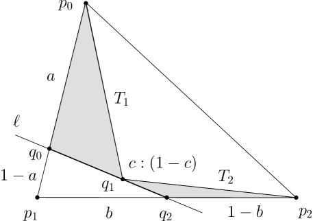
Figure 2. Characterization of $\Gamma$

Theorem 2.2.

With the above notation

$$\sqrt[3]{\mathrm{A}(T_{1})}+\sqrt[3]{\mathrm{A}(T_{2})}\leq\sqrt[3]{\mathrm{A}(T)}-\sqrt[3]{\mathrm{A}(T)}\frac{1}{3}(a-b)^{2}.$$

Proof.

Let $c$ be a number between $0$ and $1$ so that $q_{1}$ divides the segment $[q_{0},q_{2}]$ in ratio $c:(1-c)$. Then, writing $\mathrm{A}(xyz)$ for the area of the triangle with vertices $x,y,z$,

$$\mathrm{A}(p_{0}q_{0}q_{1})=a\mathrm{A}(p_{0}p_{1}q_{1})=ac\mathrm{A}(p_{0}p_{1}q_{2})=abc\mathrm{A}(p_{0}p_{1}p_{2}),$$

showing $\mathrm{A}(T_{1})=abc\mathrm{A}(T)$. Similarly, $\mathrm{A}(T_{2})=(1-a)(1-b)(1-c)\mathrm{A}(T).$ Hence we have to prove the following fact: $0\leq a,b,c\leq 1$ implies

(2.3) $$1-\sqrt[3]{abc}-\sqrt[3]{(1-a)(1-b)(1-c)}\geq\frac{1}{3}(a-b)^{2}.$$

Denote $Q$ the left hand side of (2.3). By computing the derivative of $Q$ with respect to $c$ yields that for fixed $a$ and $b$, $Q$ is minimal when

$$c=\frac{\sqrt{ab}}{\sqrt{ab}+\sqrt{(1-a)(1-b)}}\,.$$

It is easy to see that with this $c$

$$\sqrt[3]{abc}+\sqrt[3]{(1-a)(1-b)(1-c)}=\left(\sqrt{ab}+\sqrt{(1-a)(1-b)}\right)^{2/3}.$$

Now, denote $\left(\sqrt{ab}+\sqrt{(1-a)(1-b)}\right)^{2}$ by $1-u$, so

$$u=a+b-2ab-2\sqrt{ab(1-a)(1-b)}.$$

We claim that $u\geq(a-b)^{2}$: this is the same as

$$a-a^{2}+b-b^{2}\geq 2\sqrt{(a-a^{2})(b-b^{2})},$$

which is just the inequality between the arithmetic and geometric means for the numbers $a-a^{2},b-b^{2}\geq 0$. Therefore, using $u\leq 1$,

$$Q\geq 1-(1-u)^{1/3}\geq\frac{1}{3}\,u\geq\frac{1}{3}\,(a-b)^{2}.\qed$$

Theorems 2.1 and 2.2 imply the following

Corollary 2.2.

If $q_{1}\in\Gamma$ and $\ell$ is tangent to $\Gamma$ at $q_{1}$, then with the above notations, $a=b$.

It is clear that the underlying triangle $T$ can be chosen arbitrarily, since an affine transformation does not influence the value of $L_{n}$. Our standard model for $T$ is the one with $p_{0}=(0,1)$, $p_{1}=(0,0)$, $p_{2}=(1,0)$ as the vertices of $T$. In this case the special parabola $\Gamma$ has equation $\sqrt{x}+\sqrt{y}=1$.

3. Other models

There are several choices for the underlying finite set $X$. For instance, consider the lattice $\frac{1}{t}{\mathbb{Z}^{2}}$ where ${\mathbb{Z}^{2}}$ is the usual lattice in $\mathbb{R}^{2}$ and $t>0$ is large, and set $X=T\cap\frac{1}{t}{\mathbb{Z}^{2}}$. Clearly, $n:=|X|\approx\mathrm{A}(T)t^{2}$ as $t\to\infty$. Write $Y_{n}\subset X$ for a longest convex chain in $T$. It is shown in [5] that, as $t\to\infty$ (or $n\to\infty$),

(3.1) $$|Y_{n}|=\frac{6}{(2\pi)^{2/3}}\sqrt[3]{t^{2}\mathrm{A}(T)}(1+o(1))=\frac{6}{(2\pi)^{2/3}}n^{1/3}(1+o(1)).$$

This result is analogous to Theorem 1.1, except that in the lattice case the value of the constant is known to be $6/{(2\pi)^{2/3}}$, while in the present paper only the existence of the limit $\alpha$ is shown, together with $1.5<\alpha<3.5$, see Section 4. This is similar to the longest increasing subsequence problem, [1], where it is easy to see that the expectation is of order $\sqrt{n}$, but proving the precise asymptotic formula $2\sqrt{n}(1+o(1))$ turned out to be difficult, cf. [8] and [12]. In our case, numerical experiments suggest that $\alpha=3$ and we venture to conjecture that this is the actual value of $\alpha$.

More generally, let $K\subset\mathbb{R}^{2}$ be a convex compact set with nonempty interior, and set $X_{t}=K\cap\frac{1}{t}{\mathbb{Z}^{2}}$. A set $Y\subset X_{t}$ is said to be in convex position if no point of $Y$ lies in the convex hull of the others. In other words, the convex polygon $\textrm{conv}\;Y$ has exactly $|Y|$ vertices. Let $Y_{t}$ be a maximum size subset of $X_{t}$ which is in convex position and set $m(K,t)=|Y_{t}|$. It is shown in [5] that

(3.2) $$m(K,t)=\frac{3}{(2\pi)^{2/3}}\mathrm{A}^{*}(K)t^{2/3}(1+o(1))$$

where $\mathrm{A}^{*}(K)$ denotes the supremum (actually, maximum) of the affine perimeter that a convex subset of $K$ can have. The main difficulty lies in the case of triangles, that is, proving (3.1).

These results can be extended, quite easily, to the present case when $X_{n}$ is a random sample of $n$ uniform independent points from $K$. For instance, writing $Y_{n}$ for the maximum size subset of $X_{n}$ in convex position, one can show the following.

Theorem 3.1.

Under the above conditions

$$\lim_{n\rightarrow\infty}n^{-1/3}\mathbb{E}|Y_{n}|=\frac{\alpha\mathrm{A}^{*}(K)}{2\root 3 \of{A(K)}}.$$

Here $\alpha$ is the constant from Theorem 1.1.

One can also prove that $\textrm{conv}\;Y_{n}$ has a limit shape, namely, the unique convex subset of $K$ whose affine perimeter is equal to $\mathrm{A}^{*}(K)$. The proofs are almost identical to those used in [5], so we do not repeat them here, instead we rather explain what is different and more interesting.

Another random model is when $X$ comes from a homogeneous planar Poisson process $X(n)$ of intensity $n/\mathrm{A}(T)$. Given a domain $D$ in the plane, $m(D)=|X(n)\cap D|$, the number of points in $D$, has Poisson distribution with parameter $\lambda=n\mathrm{A}(D)/\mathrm{A}(T)$, i.e.

$$\mathbb{P}\big{(}m(D)=k\big{)}=e^{-\lambda}\lambda^{k}/k!\;.$$

We can also think of the Poisson model as follows: for a domain $D$, we first pick a random number $m$ according to the corresponding Poisson distribution, and then choose $m$ random, independent, uniform points in $D$. The advantage of the Poisson model is that the number of points of $X(n)$ in disjoint domains are independent random variables, unlike in the uniform model.

As is well known, the uniform model $X_{n}$ and the Poisson model $X(n)$ behave very similarly. In particular, Theorems 1.1, 1.2, and 1.3 remain valid for the Poisson model as well, with essentially the same quantitative estimates. The proofs are quite standard, and we do not go into the details. Actually, the proof of Theorem 1.3 is simpler in the Poisson model since there the subtriangles behave the same way as any other triangle.

The longest increasing subsequence problem has been almost completely solved by now, see [1]. In this respect, our results only constitute the first, and perhaps the simplest, steps in understanding the random variable $L_{n}$.

4. Expectation

The main target of this section is to prove of Theorem 1.1. We also establish upper and lower bounds for the constant involved.

Proof of Theorem 1.1.

We start with an upper bound on $\mathbb{E}L_{n}$:

(4.1) $$\limsup_{n\rightarrow\infty}\frac{\mathbb{E}L_{n}}{\sqrt[3]{n}}\leq\sqrt[3]{2}e=3.4248\dots.$$

It is shown in [3], equation (5.3) (cf. [4] as well) that the probability of $k$ uniform independent random points in $T$ forming a convex chain is

$$\frac{2^{k}}{k!\,(k+1)!}\;.$$

Therefore the probability that a convex chain of length $k$ exists is at most ${n\choose k}{2^{k}}/(k!\,(k+1)!)$. In other words

$$\mathbb{P}(L_{n}\geq k)\leq{n\choose k}\frac{2^{k}}{k!\,(k+1)!}\;.$$

We use this estimate and Stirling’s formula to bound $\mathbb{E}L_{n}$. Assume $\gamma>\sqrt[3]{2}e$. Then

$$\mathbb{E}L_{n} =\sum_{k=0}^{n}\mathbb{P}(L_{n}>k)\leq\sum_{k=0}^{n}\mathbb{P}(L_{n}\geq k)$$

$$\leq\gamma\sqrt[3]{n}+\sum_{k>\gamma\sqrt[3]{n}}\mathbb{P}(L_{n}\geq k)$$

$$\leq\gamma\sqrt[3]{n}+\sum_{k>\gamma\sqrt[3]{n}}{n\choose k}\frac{2^{k}}{k!\,(k+1)!}$$

$$\leq\gamma\sqrt[3]{n}+\sum_{k>\gamma\sqrt[3]{n}}\frac{(2n)^{k}}{(k!)^{3}}$$

$$\leq\gamma\sqrt[3]{n}+\sum_{k>\gamma\sqrt[3]{n}}\frac{1}{\sqrt{(2\pi\gamma)^{3}n}}\left(\frac{2\,e^{3}}{\gamma^{3}}\right)^{k}$$

$$\leq\gamma\sqrt[3]{n}+n^{-1/2}C,$$

where $C=\gamma^{3}/(\gamma^{3}-2e^{3})$ is a positive constant. Since this holds for arbitrary $\gamma>\sqrt[3]{2}\,e$, (4.1) is proved.

Next we establish a lower bound for $\mathbb{E}L_{n}$. We use the second half of Corollary 2.1 with $t=2\mathrm{A}(T)/n$. So we have triangles $T_{i}$ of area $t$ for $1\leq i\leq k-1$, and the last triangle $T_{k}$ of area less than $t$. By (2.1) $k\geq\sqrt[3]{n/2}$. Let $X_{n}$ be the uniform independent sample from $T$. Let $x_{i}$ be a point of $T_{i}\cap X_{n}$, provided that $T_{i}\cap X_{n}\neq\emptyset$. The collection of such $x_{i}$’s forms a convex chain. Hence the expected length of the longest convex chain is at least the expected number of non-empty triangles $T_{i}$, so

$$\mathbb{E}L_{n}\; \geq\;\sum_{1}^{k}\mathbb{P}\big{(}T_{i}\cap X_{n}\neq\emptyset\big{)}\;\geq\;(k-1)\left(1-\left(1-\frac{2}{n}\right)^{n}\right)$$

$$\geq\left(\sqrt[3]{\frac{n}{2}}-1\right)\,\left(1-e^{-2}\right)\approx 0.6862\,n^{1/3}.$$

What we have proved so far is that

$$\underline{\alpha}=\liminf_{n\rightarrow\infty}n^{-1/3}\mathbb{E}L_{n}>0.6862,\mbox{ and }\overline{\alpha}=\limsup_{n\rightarrow\infty}n^{-1/3}\mathbb{E}L_{n}<3.4249.$$

We show next that the limit exists. Suppose on the contrary that $\underline{\alpha}<\overline{\alpha}$.

The idea of the proof is to use the second half of Corollary 2.1 again, with the longest convex chain in the small triangles having length close to the limsup , while in the large triangle, $\mathbb{E}L_{n}$ is close to the liminf. For convenience, we suppose that $A(T)=1.$

Choose a large $n$ with $\mathbb{E}L_{n}\geq(1-\varepsilon)\,\overline{\alpha}\sqrt[3]{n}$, and an $N$ much larger than $n$ with $\mathbb{E}L_{N}\leq(1+\varepsilon)\,\underline{\alpha}\sqrt[3]{N}$. Here $\varepsilon$ is a suitably small positive number. Define $n_{1}$ so that the equation $n=n_{1}-\sqrt{n_{1}\log n_{1}}$ holds.

Choose $N$ uniform, independent random points from triangle $T$. Define $t=n_{1}/N$. Hence the expected number of points in a triangle (contained in $T$) of area $t$ is $n_{1}$.

Apply the second half of Corollary 2.1 with this $t$. Then the number of triangles, $k$, satisfies $k>\sqrt[3]{N/n_{1}}$.

Denote by $k_{i}$ the number of points in $T_{i}$, and by $\mathbb{E}L^{i}$ the expectation of the length of the longest convex chain in $T_{i}$. Clearly $k_{i}$ has binomial distribution with mean $n_{1}$, except for the last triangle where the mean is less than $n_{1}$.

Since the union of convex chains in the triangles $T_{i}$ is a convex chain in $T$ between $(0,0)$ and $(1,1)$, by estimate (2.1) we have

$$\mathbb{E}L_{N} \geq\sum_{i\leq k}\mathbb{E}L^{i}\;\geq\;\sum_{i\leq k-1}\mathbb{P}(k_{i}>n)\mathbb{E}L_{n}$$

$$\geq\sum_{i\leq k-1}\left(1-n_{1}^{-1/2}\right)(1-\varepsilon)\,\overline{\alpha}\sqrt[3]{n}$$

$$\geq\left(\sqrt[3]{N/n_{1}}-1\right)\left(1-n_{1}^{-1/2}\right)(1-\varepsilon)\,\overline{\alpha}\sqrt[3]{n}$$

$$=\overline{\alpha}\,\sqrt[3]{N}(1-\varepsilon)\left(1-n_{1}^{-1/2}\right)\left(\sqrt[3]{n/n_{1}}-\sqrt[3]{n/N}\right)$$

$$\geq\overline{\alpha}\,\sqrt[3]{N}(1-2\varepsilon),$$

where the last inequality holds if $n$ is chosen large enough and $N$ is chosen even larger with $n/N$ very small. Thus $(1+\varepsilon)\,\underline{\alpha}\geq(1-2\varepsilon)\,\overline{\alpha}$ which, for small enough $\varepsilon$, contradicts our assumption $\underline{\alpha}<\overline{\alpha}$. ∎

Remark. The lower bound $\mathbb{E}L_{n}\geq 0.6862\,n^{1/3}$ is probably the easiest to prove. A better estimate, also mentioned by Enriquez [7], can be established as follows. Assume $T$ is the standard triangle and let $D$ denote the domain of $T$ lying above $\Gamma$. Then $\mathrm{A}(D)=1/3$, so the expected number of points in $D$ is $2n/3$, and the number of points is concentrated around this expectation. The affine perimeter of $D$ is $2\sqrt[3]{1/2}$ (see [3]), and a classical result of Rényi and Sulanke [9] yields that expected number of vertices of $\textrm{conv}(D\cap X_{n})$ is about

$$\Gamma\left(\frac{5}{3}\right)\sqrt[3]{\frac{2}{3}}\left(\frac{1}{3}\right)^{-1/3}2\sqrt[3]{1/2}\,\sqrt[3]{2n/3}\approx 1.5772\,\sqrt[3]{n}$$

Since most vertices are located next to the parabola, the majority of them form a convex chain, and so

(4.2) $$\liminf_{n\rightarrow\infty}\frac{\mathbb{E}L_{n}}{\sqrt[3]{n}}\geq 1.5772\dots.$$

This sketch can be completed with standard tools. From now on, we will use this estimate. Also, $\alpha$ will always refer to the limit constant of Theorem 1.1.

5. Concentration results for $\mathbb{E}L_{n}$

The concentration results proved here are consequences of Talagrand’s inequality from [10] which says the following. Suppose $Y$ is a real-valued random variable on a product probability space $\Omega^{\otimes n}$, and that $Y$ is 1-Lipschitz with respect to the Hamming distance, meaning that

$$|Y(x)-Y(y)|\leq 1$$

whenever $x$ and $y$ differ in one coordinates. Moreover assume that $Y$ is $f$-certifiable. This means that there exists a function $f:\mathbb{N}\rightarrow\mathbb{N}$ with the following property: for every $x$ and $b$ with $Y(x)\geq b$ there exists an index set $I$ of at most $f(b)$ elements, such that $Y(y)\geq b$ holds for every $y$ agreeing with $x$ on $I$. Let $m$ denote the median of $Y$. Then for every $s>0$ we have

$$\mathbb{P}(Y\leq m-s)\leq 2\,\mathrm{exp}\left(\frac{-s^{2}}{4f(m)}\right)$$

and

$$\mathbb{P}(Y\geq m+s)\leq 2\,\mathrm{exp}\left(\frac{-s^{2}}{4f(m+s)}\right).$$

When applied to $L_{n}$, these inequalities prove concentration about the median, to be denoted by $m_{n}$. Theorem 1.2 concerns the mean of $L_{n}$. However, concentration ensures that the mean and the median are not far apart, in fact, $\lim n^{-1/3}m_{n}=\alpha$. First we need a lower bound on $m_{n}$.

Lemma 5.1.

Suppose that $\log n>25$. Then

$$m_{n}\geq\sqrt[3]{3n/\log n}.$$

Since this is a special case of Lemma 6.1 from the next section, the proof will be given there.

Proof of Theorem 1.2.

The statement cries out for the application of Talagrand’s inequality. The random variable $L_{n}$ satisfies the conditions with $f(b)=b$, since fixing the coordinates of a maximal chain guarantees that the length will not decrease, and changing one coordinate changes the length of the maximal chain by at most one. Write $m=m_{n}$ for the median in the present proof. Setting $s=\beta\sqrt{m\log m}$ where $\beta$ is an arbitrary positive constant, we have

$$\mathbb{P}\big{(}|L_{n}-m|\geq\beta\sqrt{m\log m}\,\big{)} <4\exp\left\{\frac{-\beta^{2}m\log m}{4(m+\beta\sqrt{m\log m})}\right\}$$

$$=4\exp\left\{\frac{-\beta^{2}\log m}{4(1+\beta\sqrt{m^{-1}\log m})}\right\}$$

Define now $\beta_{0}=c\sqrt{m/\log m}$ with a constant $c>0$, which will be fixed at the end of the proof in order to give the correct estimate. If $\beta\leq\beta_{0}$, then $\beta\sqrt{m^{-1}\log m}\leq c$, and the denominator in the exponent is at most $4(1+c)$. Thus

(5.1) $$\mathbb{P}\big{(}|L_{n}-m|\geq\beta\sqrt{m\log m}\,\big{)}<4m^{\frac{-\beta^{2}}{4(1+c)}}.$$

On the other hand, for $\beta>\beta_{0}$ we have

(5.2) $$\mathbb{P}\big{(}|L_{n}-m|\geq\beta\sqrt{m\log m}\,\big{)} <\mathbb{P}\big{(}|L_{n}-m|\geq\beta_{0}\sqrt{m\log m}\,\big{)}$$

$$=4\exp\left(-m\,\frac{c^{2}}{4(1+c)}\right).$$

Next, we compare the median and the expectation of $L_{n}$.

$$|\mathbb{E}L_{n}-m|\leq\mathbb{E}|L_{n}-m|=\int_{0}^{\infty}\;\mathbb{P}(|L_{n}-m|>x)dx.$$

The range of $L_{n}$ is $[1,n]$, so the integrand is $0$ if $x>n$. Substitute $x=\beta\sqrt{m\log m}$, and divide the integral into two parts at $\beta_{0}$:

$$|\mathbb{E}L_{n}-m|\leq 4\sqrt{m\log m}(I_{1}+I_{2}),$$

where

(5.3) $$I_{1}=\int_{0}^{\beta_{0}}m^{-\beta^{2}/4(1+c)}d\beta<\int_{0}^{\infty}m^{-\beta^{2}/4(1+c)}d\beta=\sqrt{\frac{\pi(1+c)}{\log m}},$$

and

(5.4) $$I_{2}=\int_{\beta_{0}}^{n/\sqrt{m\log m}}\exp\left(-m\,\frac{c^{2}}{4(1+c)}\right)d\beta<n\exp\left(-m\,\frac{c^{2}}{4(1+c)}\right).$$

By Lemma 5.1, $n<m^{4}$, so $I_{2}<m^{4}\exp(-m\,c^{2}/4(1+c))$. Since $m_{n}$ goes to infinity as $n$ increases (again by Lemma 5.1), the bound on $I_{2}$ is eventually much smaller than the one on $I_{1}$:

$$|\mathbb{E}L_{n}-m| \leq 4\sqrt{m\log m}(I_{1}+I_{2})$$

(5.5) $$<4\sqrt{\pi(1+c)m}+4\sqrt{m\log m}\,m^{4}\exp\left(-m\,\frac{c^{2}}{4(1+c)}\right)$$

$$\leq 5\sqrt{\pi(1+c)}\sqrt{m}$$

for all large enough $n$. Hence $\mathbb{E}L_{n}$ is of the same order of magnitude as $m_{n}$, and we obtain

(5.6) $$\lim n^{-1/3}\mathbb{E}L_{n}=\lim n^{-1/3}m_{n}=\alpha.$$

For fixed $\gamma$ and for large enough $n$, (5) implies

$$\mathbb{P}\big{(}|L_{n}-\mathbb{E}L_{n}|>\gamma\sqrt{\log n}\;n^{1/6}\big{)}$$

$$\leq\mathbb{P}\big{(}|L_{n}-m|>\gamma\sqrt{\log n}\;n^{1/6}-|\mathbb{E}L_{n}-m|\,\big{)}$$

$$\leq\mathbb{P}\big{(}|L_{n}-m|>\gamma\sqrt{\log n}\;n^{1/6}-5\sqrt{\pi(1+c)}\sqrt{m}\,\big{)}.$$

Using $m_{n}\leq 3.43n^{1/3}$ from (4.1) and (5.6), it is easy to see that

$$\gamma\sqrt{\log n}\;n^{1/6}-5\sqrt{\pi(1+c)\,m} \geq\gamma\sqrt{m}\left(\sqrt{\frac{3\log m-\log 41}{3.43}}-\frac{5\sqrt{\pi(1+c)}}{\gamma}\right)$$

$$\geq\gamma\sqrt{\frac{3}{3.44}}\sqrt{m\log m}.$$

Since for large enough $n$, $\gamma\sqrt{3/3.44}<\beta_{0}=c\sqrt{m/\log m}$, (5.1) finally implies

$$\mathbb{P}\big{(}|L_{n}-\mathbb{E}L_{n}|\geq\gamma\sqrt{\log n}\;n^{1/6}\big{)}$$

$$\leq\mathbb{P}\big{(}|L_{n}-m|\geq\gamma\sqrt{\frac{3}{3.44}}\sqrt{m\log m}\,\big{)}$$

$$\leq 4m^{-3\gamma^{2}/13.76(1+c)}\leq n^{-\gamma^{2}/14}$$

with (5.6) and the choice of $c=0.01$. ∎

Remark. The constant in the exponent is far from being best possible. We have made no attempt to find its optimal value. In general, Talagrand’s inequality is too general to give the precise concentration, see Talagrand’s comments on this in [10].

6. Subtriangles

For the proof of Theorem 1.3 we need to consider subtriangles $S$ of $T$, that is, triangles of the form $S=\textrm{conv}\;\{a,b,c\}$ with $a,b,c\in T$, while $X_{n}$ is still a random sample from $T$. We will need to estimate the concentration of the longest convex chain from $X_{n}$ in $S$. Since this random variable depends only on the relative area of $S$, we may and do assume that $T$ is the standard triangle and $S=\textrm{conv}\{(0,\sqrt{s}),(0,0),(\sqrt{s},0)\}$. Thus $\mathrm{A}(S)=s/2$. Write $L_{s,n}$ for the length of the longest convex chain in $S$ from $(0,\sqrt{s})$ to $(\sqrt{s},0)$, and $m_{s,n}$ for its median. In the following statements, we consider the situation when $sn/2$, the expected number of points from $X_{n}$ in $S$, tends to infinity.

As in the proof of Theorem 1.2, we need two estimates: a lower bound for the median guarantees that the mean and the median are close to each other, while an upper bound for the expectation (or for the median) is needed for deriving the inequality in terms of $n$. Here comes the lower bound; the case $s=1$ is Lemma 5.1.

Lemma 6.1.

Suppose that $\log(ns)>25$. Then

$$m_{s,n}\geq\sqrt[3]{3ns/\log(ns)}.$$

Proof.

Set $t=(\mathrm{A}(S)\log(ns))/(3ns)$, and apply the second half of Corollary 2.1 to the triangle $S$. The number of triangles is $k$ with

$$\sqrt[3]{3ns/\log(ns)}<k\leq\sqrt[3]{3ns/\log(ns)}+1.$$

For any $i\in\{1,\dots,k$}, the probability that $T_{i}$ contains no point of $X_{n}$ is

$$\mathbb{P}(T_{i}\cap X_{n}=\emptyset) \leq\left(1-\frac{\log(ns)}{3ns}\right)^{n}$$

$$<\exp\left(\frac{-\log(ns)}{3s}\right)=(ns)^{-1/3s}<(ns)^{-1/3}.$$

Hence the union bound yields

$$\mathbb{P}\big{(}L_{n,s}>\sqrt[3]{3ns/\log(ns)}\,\big{)} \geq 1-\mathbb{P}(T_{i}\cap X_{n}=\emptyset\mbox{ for some }i\leq k)$$

$$\geq 1-k\,(ns)^{-1/3}$$

$$\geq 1-\big{(}\sqrt[3]{3/\log(ns)}+(ns)^{-1/3}\big{)},$$

which is greater than $1/2$ by the assumption. ∎

Obtaining an upper bound for the mean is slightly more delicate; note that in the Lemma below $s$ need not be fixed.

Lemma 6.2.

Assume $ns\to\infty$. Then

$$\lim\,(ns)^{-1/3}\mathbb{E}L_{s,n}=\alpha$$

where $\alpha$ is the same constant as in Theorem 1.1.

Proof.

Take any $\varepsilon>0$ and choose $N_{0}$ (depending on $\varepsilon$) so large that for every $k\geq N_{0}$, $(1-\varepsilon)\alpha<\mathbb{E}L_{k}\,k^{-1/3}<(1+\varepsilon)\alpha$. The random variable $K=|X_{n}\cap S|$ has binomial distribution with mean $ns$. When $ns$ is large enough, $ns-\sqrt{ns\log ns}\geq N_{0}$, and we use (2.1) for a lower estimate:

$$\mathbb{E}L_{s,n} =\sum_{k=0}^{n}\mathbb{P}(K=k)\mathbb{E}L_{k}$$

$$\geq\mathbb{P}(K>ns-\sqrt{ns\log ns})(1-\varepsilon)\,\alpha\,(ns-\sqrt{ns\log ns})^{1/3}$$

$$\geq(1-(ns)^{-1/2})(1-\varepsilon)\,\alpha\,(ns-\sqrt{ns\log ns})^{1/3}$$

$$\geq(1-2\varepsilon)\,\alpha\,(ns)^{1/3}.$$

For the upper bound, Jensen’s inequality applied to $\sqrt[3]{x}$ comes in handy:

$$\mathbb{E}L_{s,n} =\sum_{k=0}^{n}\mathbb{P}(K=k)\mathbb{E}L_{k}$$

$$\leq N_{0}\,\mathbb{P}(K<N_{0})+\sum_{k=N_{0}}^{n}\mathbb{P}(K=k)\mathbb{E}L_{k}$$

$$\leq N_{0}\,+\sum_{k=N_{0}}^{n}\mathbb{P}(K=k)\,(1+\varepsilon)\,\alpha\,\sqrt[3]{k}$$

$$\leq N_{0}\,+\mathbb{P}(K\geq N_{0})\,(1+\varepsilon)\,\alpha\,\left(\sum_{k=N_{0}}^{n}\frac{\mathbb{P}(K=k)}{\mathbb{P}(K\geq N_{0})}\ k\right)^{1/3}$$

$$\leq N_{0}\,+\mathbb{P}(K\geq N_{0})^{2/3}\,(1+\varepsilon)\,\alpha\,(\mathbb{E}\,K)^{1/3}$$

$$\leq N_{0}+(1+\varepsilon)\,\alpha\,(ns)^{1/3}\leq(1+2\varepsilon)\,\alpha\,(ns)^{1/3}.\qed$$

Next, we derive the strong concentration property of $L_{s,n}$, the analogue of Theorem 1.2.

Theorem 6.1.

Suppose $\tau$ is a constant with $0\leq\tau<1$. Then for every $\gamma>0$ there exists a constant $N$, such that for every $n>N$ and every $s\geq n^{-\tau}$,

$$\mathbb{P}\big{(}|L_{s,n}-\mathbb{E}L_{s,n}|>\gamma\sqrt{\log ns}\;(ns)^{1/6}\big{)}<(ns)^{-\gamma^{2}/14}.$$

Proof.

This proof is almost identical with that of Theorem 1.2. Since $L_{s,n}$ is a random variable on $T^{\otimes n}$, we can apply Talagrand’s inequality with the certificate function $f(b)=b$ in the same way as in the proof of Theorem 1.2. Write again $m$ for $m_{s,n}$, the median of $L_{s,n}$. Define $\beta_{0}=c\sqrt{m/\log m}$ with $c=0.01$, then the estimates (5.1) and (5.2) remain valid with $L_{s,n}$ in place of $L_{n}$. Just as before,

$$|\mathbb{E}L_{s,n}-m| \leq\mathbb{E}|L_{s,n}-m|=\int_{0}^{\infty}\;\mathbb{P}(|L_{s,n}-m|>x)dx$$

$$=4\sqrt{m\log m}(I_{1}+I_{2})$$

where $I_{1}$ and $I_{2}$ are defined the same way as in (5.3) and (5.4). Moreover, $I_{1}$ satisfies the inequality (5.3). With $I_{2}$ we have to be a bit more careful.

Note that $s\geq n^{-\tau}$ with $\tau<1$ guarantees that Lemma 6.1 is applicable for $n>\exp(25/(1-\tau))$. As $x/\log x$ is monotone increasing for $x>e$,

$$m\geq\sqrt[3]{\frac{3ns}{\log(ns)}}\geq\sqrt[3]{\frac{3n^{1-\tau}}{(1-\tau)\log n}}>\sqrt[3]{\frac{n^{1-\tau}}{n^{(1-\tau)/2}}}=n^{(1-\tau)/6}$$

for large enough $n$, and therefore by (5.4)

$$I_{2}<m^{6/(1-\tau)}\exp\left(-m\,\frac{c^{2}}{4(1+c)}\right)$$

where of course $6/(1-\tau)<\infty$. Lemma 6.1 implies that $m=m_{s,n}\rightarrow\infty$, thus the bound on $I_{2}$ is much smaller than the one on $I_{1}$ for large enough $n$. Therefore, just as in (5),

$$|\mathbb{E}L_{s,n}-m| \leq 4\sqrt{m\log m}(I_{1}+I_{2})$$

$$<4\sqrt{\pi(1+c)m}+4\sqrt{m\log m}\,m^{6/(1-\tau)}\exp\left(-m\,\frac{c^{2}}{4(1+c)}\right)$$

$$\leq 5\sqrt{\pi(1+c)}\sqrt{m}.$$

Hence $\mathbb{E}L_{s,n}$ is of the same order of magnitude as $m=m_{s,n}$. Since $sn\geq n^{1-\tau}\rightarrow\infty$, we can use Lemma 6.2, obtaining that for large enough $n$,

(6.1) $$m_{s,n}\leq 3.431\sqrt[3]{ns}.$$

Again for fixed $\gamma$ and for large enough $n$,

$$\mathbb{P}(|L_{s,n}-\mathbb{E}L_{s,n}|>\gamma\sqrt{\log ns}\;(ns)^{1/6})$$

$$\leq\mathbb{P}(|L_{s,n}-m|>\gamma\sqrt{\log ns}\;(ns)^{1/6}-|\mathbb{E}L_{s,n}-m|)$$

$$\leq\mathbb{P}(|L_{s,n}-m|>\gamma\sqrt{\log ns}\;(ns)^{1/6}-5\sqrt{\pi(1+c)}\sqrt{m}),$$

and by (6.1),

$$\gamma\sqrt{\log ns}\;(ns)^{1/6}-5\sqrt{\pi(1+c)}\sqrt{m} \geq\gamma\sqrt{\frac{3}{3.44}}\sqrt{m\log m}.$$

Since for large enough $n$, $\gamma\sqrt{3/3.44}<\beta_{0}=c\sqrt{m/\log m}$, (5.1) applied to $L_{s,n}$ and (6.1) finally implies

$$\mathbb{P}\big{(}|L_{s,n}-\mathbb{E}L_{s,n}|\geq\gamma\sqrt{\log ns}\;(ns)^{1/6}\big{)}$$

$$\leq\mathbb{P}\big{(}|L_{s,n}-m|\geq\gamma\sqrt{\frac{3}{3.44}}\sqrt{m\log m}\,\big{)}$$

$$\leq 4m^{-3\gamma^{2}/13.76(1+c)}\leq(ns)^{-\gamma^{2}/14}.\qed$$

Remark. The proof also yields that for any $0<A<B<\infty$, there exists $N$ (depending on $A$ and $B$ only), such that the inequality of Theorem 6.1 holds for any $\gamma\in[A,B]$ and for every $n>N$.

7. Geometric lemmas

For the proof of Theorem 1.3 we need further preparations. We start by assuming that $K$ is a convex compact set in the plane and $A(K)>0$, and $\widetilde{X}_{n}$ is a random sample of $n$ uniform and independent points from $K$. We need to estimate the probability that $\widetilde{X}_{n}$ is in convex position, that is, no point of $\widetilde{X}_{n}$ is contained in the convex hull of the others. We denote this probability by $\mathbb{P}(\widetilde{X}_{n}\mbox{ convex in }K)$.

Lemma 7.1.

If $K$ is as above,

$$\mathbb{P}(\widetilde{X}_{n}\mbox{ {\rm convex in} }K)<\left(\frac{240}{n^{2}}\right)^{n}.$$

Proof..

Let $P$ be the smallest area parallelogram containing $K$. As is well known, $A(P)\leq 2A(K)$. Let $X_{n}^{*}$ be a random sample of $n$ uniform and independent points from $P$. In this case a (surprisingly exact) result of Valtr [11] says that

$$\mathbb{P}(X_{n}^{*}\mbox{ convex in }P)=(n!)^{-2}{{2n-2}\choose{n-1}}^{2}.$$

Now we have

$$\mathbb{P}(\widetilde{X}_{n}\mbox{ convex in }K) =\mathbb{P}(X_{n}^{*}\mbox{ convex in }P\,|\,X_{n}^{*}\subset K)$$

$$=\frac{\mathbb{P}(X_{n}^{*}\mbox{ convex in }P\mbox{ and }X_{n}^{*}\subset K)}{\mathbb{P}(X_{n}^{*}\subset K)}$$

$$\leq\frac{\mathbb{P}(X_{n}^{*}\mbox{ convex in }P)}{\mathbb{P}(X_{n}^{*}\subset K)}$$

$$=(n!)^{-2}{{2n-2}\choose{n-1}}^{2}\left(\frac{A(P)}{A(K)}\right)^{n}<\left(\frac{240}{n^{2}}\right)^{n},$$

where the last step is a straightforward estimate. ∎

¿From now on we work exclusively with the standard triangle $T$.

Assume next that $K$ is a convex subset of the triangle $T$, and let $X_{n}$ be random sample of $n$ uniform and independent points from $T$. We define $M(K,n)$ as the random variable

$$M(K,n)=\max\{|Y|:Y\subset X_{n}\cap K\mbox{ is in convex position}\}.$$

¿From Theorem 3.1 it is not hard to determine what the asymptotic expectation of $M(K,n)$ is. But what we need is that $M(K,n)$ is large with small probability. This is the content of the next lemma.

Lemma 7.2.

Let $K$ be a convex subset of $T$. Then for any positive integers $n$ and $\mu$ satisfying $1920\,e^{2}\,A(K)\,n\leq\mu^{3}$,

$$\mathbb{P}(M(K,n)\geq\mu)\leq\mu^{3}2^{-\mu}+n2^{-\mu^{3}/(480e)}.$$

Proof..

If $M(K,n)\geq\mu$, then $K\cap X_{n}$ contains a subset of size $\mu$ which is in convex position. Lemma 7.1 and the union bound imply that

$$\mathbb{P}\big{(}M(K,n)\geq\mu\big{|}|K\cap X_{n}|=k\big{)}\leq{k\choose\mu}\left(\frac{240}{\mu^{2}}\right)^{\mu}\leq\left(\frac{240\,e\,k}{\mu^{3}}\right)^{\mu}.$$

The random variable $|K\cap X_{n}|$ has binomial distribution. Thus we have

$$\mathbb{P}(M(K,n)\geq\mu)$$

$$=\sum_{k=\mu}^{n}\mathbb{P}\big{(}M(K,n)\geq\mu\big{|}|K\cap X_{n}|=k\big{)}{n\choose k}(2A(K))^{k}(1-2A(K))^{n-k}$$

$$\leq\sum_{k=\mu}^{n}\min\left\{1,\left(\frac{240\,e\,k}{\mu^{3}}\right)^{\mu}\right\}{n\choose k}(2A(K))^{k}(1-2A(K))^{n-k}$$

$$=\sum_{k<k_{0}}[..]+\sum_{k=k_{0}}^{n}[..].$$

Here we choose $k_{0}$ to be equal to $\mu^{3}/(480e)$. Then

$$\sum_{k<k_{0}}[..]\leq\sum_{k<k_{0}}\left(\frac{240\,e\,k_{0}}{\mu^{3}}\right)^{\mu}<k_{0}2^{-\mu}<\mu^{3}2^{-\mu}.$$

Since ${n\choose k}(2A(K))^{k}(1-2A(K))^{n-k}$ is decreasing for $k>2A(K)n$, and the condition on $\mu$ guarantees that $k_{0}>2A(K)n$,

$$\sum_{k>k_{0}}[..] \leq n{n\choose k_{0}}(2A(K))^{k_{0}}(1-2A(K))^{n-k_{0}}$$

$$\leq n\left(\frac{ne}{k_{0}}\right)^{k_{0}}(2A(K))^{k_{0}}=n\left(\frac{2eA(K)n}{k_{0}}\right)^{k_{0}}$$

$$< n2^{-k_{0}}=n2^{-\mu^{3}/(480e)}.$$

∎

For the proof of Theorem 1.3 we will consider other parabolas that are similar to $\Gamma$. Let $\Gamma_{r}$ be the parabola defined by the equation $\sqrt{x}+\sqrt{y}=\sqrt{1+r}$ where the parameter $r\in(-1,3)$. The graph of $\Gamma_{r}$ is the homothetic copy of $\Gamma$ with ratio of homothety $1+r$, and center of homothety at the origin, see Figure 3 a). Assume the point $(a,b)$ is on $\Gamma$. Then the point $((1+r)a,(1+r)b)$ is on $\Gamma_{r}$, and the tangent line to this point on $\Gamma_{r}$ is given by the equation

$$\frac{x}{\sqrt{a}}+\frac{y}{\sqrt{b}}=1+r.$$

It follows that the distance between parallel tangent lines to $\Gamma$ and $\Gamma_{r}$ is

(7.1) $$\frac{|r|}{\sqrt{\frac{1}{a}+\frac{1}{b}}}\leq\frac{|r|}{\sqrt{8}}.$$

Define now

$$\rho=\sqrt{8}\varepsilon=3\sqrt{2}\gamma^{1/2}n^{-1/12}(\log n)^{1/4},$$

here $\varepsilon$ comes from Theorem 1.3. This definition immediately implies the following fact.

Proposition 7.1.

If a convex chain $C(Y)$ lies between $\Gamma_{-\rho}$ and $\Gamma_{\rho}$, then $\textrm{dist}(C(Y),\Gamma)\leq\varepsilon$.

We need one more piece of preparation. Assume $\ell$ is a tangent to $\Gamma_{r}$, at the point $q$. With the notations of Section 2, let $T_{1}$ and $T_{2}$ denote the two triangles determined by $\ell$ and $q$, see Figure 3 a). Let $X_{n}$ be a random sample of $n$ points from $T$ and let $L^{i}$ denote the length of the longest convex chain in $T_{i}$, $i=1,2$.

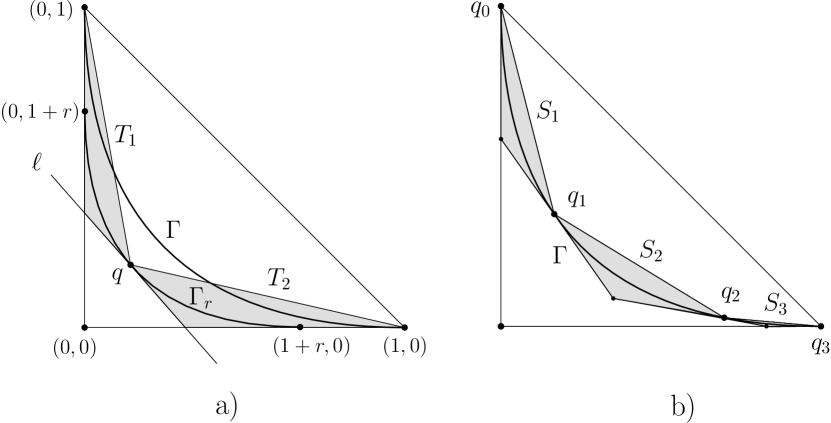
Figure 3. Convex chains far from $\Gamma$

Lemma 7.3.

For sufficiently large $n$, if $|r|\geq n^{-1/12}$, then

$$\mathbb{E}L^{1}+\mathbb{E}L^{2}\leq\mathbb{E}L_{n}-0.52\,r^{2}\sqrt[3]{n}.$$

Proof..

Let $t_{i}=2\mathrm{A}(T_{i})$ for $i=1,2$. We want to apply Theorem 2.2. It is not hard to see (using Corollary 2.2 for instance) that what is denoted by $|a-b|$ there, is equal to $|r|$ here. Consequently

(7.2) $$\sqrt[3]{t_{1}/2}+\sqrt[3]{t_{2}/2}\leq\sqrt[3]{1/2}-\sqrt[3]{1/2}\;\frac{1}{3}\,r^{2}.$$

Write $L^{i}$ for the longest convex chain in the triangle $T_{i}$. By affine invariance $L^{i}$ has the same distribution as $L_{t_{i},n}$ (from Section 6) for $i=1,2$. We need to estimate $\mathbb{E}L_{n}-(\mathbb{E}L^{1}+\mathbb{E}L^{2})$ from below.

For four points $q_{0}=(0,1)$, $q_{1}$, $q_{2}$ and $q_{3}=(1,0)$ in this order on $\Gamma$, denote by $S_{i}$ the triangle delimited by the tangents to $\Gamma$ at $q_{i-1},q_{i}$, and by the segment $[q_{i-1},q_{i}]$, $i=1,2,3$; see Figure 3 b). Choose $q_{1}$ and $q_{2}$ so that $\mathrm{A}(S_{1})=t_{1}/2$ and $\mathrm{A}(S_{2})=t_{2}/2$. Then Corollary 2.1 and (7.2) imply that

$$\sqrt[3]{\mathrm{A}(S_{3})}\geq\sqrt[3]{1/2}\;\frac{1}{3}\,r^{2}.$$

Let now $\Lambda^{i}$ denote the length of a longest chain in $S_{i}$ for $i=1,2,3$. For $i=1$ and $2$, $\Lambda^{i}$ has the same distribution as $L_{t_{i},n}$ (and as $L^{i}$). Therefore $\mathbb{E}L^{i}=\mathbb{E}L_{t_{i},n}=\mathbb{E}\Lambda^{i}$ for $i=1,2$. Further, $\Lambda^{1}+\Lambda^{2}+\Lambda^{3}\leq L_{n}$ follows from concatenating the longest convex chains in the triangles $S_{i}$. Thus we have

(7.3) $$\mathbb{E}L^{1}+\mathbb{E}L^{2}+\mathbb{E}\Lambda^{3}=\sum_{i=1}^{3}\mathbb{E}\Lambda^{i}\leq\mathbb{E}L_{n}.$$

The random variable $|X_{n}\cap S_{3}|$ has binomial distribution with mean $2A(S_{3})n$ which is at least $\kappa=(1/3)^{3}r^{6}n\geq(1/3)^{3}n^{1/2}$. Set $N=\kappa-\sqrt{\kappa\log\kappa}$. Thus we obtain that for all large enough $n$,

$$N>0.99\,\kappa=\frac{0.99}{27}r^{6}n,$$

and $N$ tends to infinity with $n$. Using the estimates (2.1) and (4.2), again for large $n$ we have

$$\mathbb{E}\Lambda^{3} \geq\mathbb{P}(|X_{n}\cap S_{3}|\geq N)\,\mathbb{E}L_{N}\geq(1-\kappa^{-1/2})\ 1.57\,N^{1/3}$$

$$\geq 1.569N^{1/3}\geq 0.52\,r^{2}\sqrt[3]{n}.$$

Hence, by (7.3)

$$\mathbb{E}L^{1}+\mathbb{E}L^{2}\leq\mathbb{E}L_{n}-0.52\,r^{2}\sqrt[3]{n}.$$

∎

8. Limit shape

After the preparations in the previous sections we finally prove Theorem 1.3, that is, all chains in $\mathcal{C}$ lie in a small neighbourhood of $\Gamma$ with high probability. Note that similar limit shape results have been proved for convex chains [4]; however, they are of different character than the present case.

We fix the constant $\gamma\geq 1$. Every result in this chapter holds for large enough $n$, depending only on $\gamma$. We will not always mention this.

For this proof we set $b=\gamma n^{1/6}\sqrt{\log n}$. The strong concentration result of Theorem 1.2 directly shows that

$$\mathbb{P}(L_{n}<\mathbb{E}L_{n}-b)\leq n^{-\gamma^{2}/14}.$$

We call a convex chain $Y\subset X_{n}$ long if its length is at least $\mathbb{E}L_{n}-b$.

We will show that all long convex chains lie between the parabolas $\Gamma_{\rho}$ and $\Gamma_{-\rho}$ with high probability, where high means $>1-n^{-\gamma^{2}/14}$. In view of Proposition 7.1 this suffices for the proof.

Let $S$ be the triangle with vertices $(0,0.1),(0,0),(0.1,0)$, and define $H$ to be the event that there is a long convex chain $Y\subset X_{n}$ having a point in $S$. We prove first the following simple fact.

Lemma 8.1.

For $n$ large enough,

$$\mathbb{P}(H)\leq n^{-\gamma^{2}/6}.$$

Proof..

Let $Y$ be a long convex chain with a point in $S$, and let $y$ be a point of $Y$ where the tangent to $C(Y)$ has slope $1$. Clearly $y\in S$. Let $Y_{1}$ be the part of $Y$ between $(0,1)$ and $y$, and $Y_{2}$ be the part between $y$ and $(1,0)$. Then $Y_{1}$ resp. $Y_{2}$ are convex chains in the triangle $S_{1}=\textrm{conv}\{(0,1),(0,0),(0.1,0)\}$ and $S_{2}=\textrm{conv}\{(0,0.1),(0,0),(1,0)\}$. As $Y$ is a long convex chain,

$$\mathbb{E}L_{n}-b\leq|Y|\leq|Y_{1}|+|Y_{2}|\leq L^{1}+L^{2},$$

where $L^{i}$ denotes the length of the maximal chain in $S_{i}$ ($i=1,2$), $|Y_{i}|\leq L^{i}$. As $n\to\infty$, the limit of $n^{-1/3}\mathbb{E}L_{n}$ resp. $n^{-1/3}\mathbb{E}L^{i}$ is $\alpha$ and $\alpha\sqrt[3]{0.1}$. This follows from Theorem 1.1 and Lemma 6.2. So $\lim n^{-1/3}(\mathbb{E}L_{n}-\mathbb{E}L^{1}-\mathbb{E}L^{2})=\alpha(1-2\sqrt[3]{0.1})>1/10$, implying that for large enough $n$

$$\mathbb{E}L_{n}-\mathbb{E}L^{1}-\mathbb{E}L^{2}>\frac{1}{10}\sqrt[3]{n}>3b=3\gamma n^{1/6}\sqrt{\log n}.$$

So we have

$$\mathbb{P}(H)\leq\mathbb{P}(L^{1}+L^{2}>\mathbb{E}L_{n}-b)$$

$$=\mathbb{P}(L^{1}+L^{2}>\mathbb{E}L^{1}+\mathbb{E}L^{2}+(\mathbb{E}L_{n}-\mathbb{E}L^{1}-\mathbb{E}L^{2})-b)$$

$$\leq\mathbb{P}(L^{1}+L^{2}>\mathbb{E}L^{1}+\mathbb{E}L^{2}+2b)\leq\sum_{i=1,2}\mathbb{P}(L^{i}>\mathbb{E}L^{i}+b).$$

The triangle $S_{i}$ is of area $1/20$ so Theorem 6.1 shows that

$$\mathbb{P}(L^{i}>\mathbb{E}L^{i}+b)=\mathbb{P}(L^{i}>\mathbb{E}L^{i}+\gamma n^{1/6}\sqrt{\log n})$$

$$\leq\mathbb{P}(L^{i}>\mathbb{E}L^{i}+\gamma\,20^{1/6}(n/20)^{1/6}\sqrt{\log n/20})$$

$$\leq\left(\frac{n}{20}\right)^{-\gamma^{2}\,20^{1/3}/14}\leq\frac{1}{2}\,n^{-\gamma^{2}/6}.\qed$$

After this first step, we estimate the probability of the existence of a long convex chain not lying between $\Gamma_{-\rho}$ and $\Gamma_{\rho}$. First, we deal with the case when the chain goes below this region.

We define a set of parabolas. Let $\triangle=n^{-1/3}\sqrt{\log n}$, $r_{i}=-\rho-i\triangle$, and

(8.1) $$G_{i}=\Gamma_{r_{i}}\mbox{ where }i=-1,0,1,\dots,g.$$

Note that $r_{i}<0$. Here we define $g$ by the conditions $G_{g}\subset S$ but $G_{i-1}$ is not contained in $S$. Thus the case when a long chain goes below $G_{g}$ is covered by Lemma 8.1. Clearly $g$ is limited by $-1<r_{g}=-\rho-g\triangle\geq-1+1/10$. Thus $g\leq n^{2/3}$, say.

The convex polygonal chains $C(Y)$ can be considered as functions defined on $[0,1]$. We extend the definition of $\Gamma_{r}$ as 0 on the interval $[1+r,1]$ if $r<0$, and consider this new “parabola” $\Gamma_{r}$ as a function defined on $[0,1]$. A parabola is said to be below, resp. above $C(Y)$ if the corresponding function is smaller (larger) than the one corresponding to $C(Y)$.

The following lemma is important.

Lemma 8.2.

There are points $q_{i,j}\in G_{i-1},\;j=1,2,\dots,J(i)$ with $J(i)\leq n^{1/3}$, such that the upper envelope of the tangent lines $\ell(q_{i,j})$ of $G_{i-1}$ at $q_{i,j}$ is a broken polygonal path lying above $G_{i}$.

Proof..

The line $\ell_{q}$, which is tangent to $G_{i-1}$ at $q\in G_{i-1}$, intersects the graph of $G_{i}$ in two points. Let $\lambda_{q}$ denote the segment connecting these two points. It is not hard to check that the length of the segment, $|\lambda(q)|$, decreases as $q$ moves away from the center point of $G_{i-1}$. A simple computation reveals that

(8.2) $$4\triangle\frac{(1+r_{i})^{2}}{(1+r_{i-1})^{2}}\leq|\lambda_{q}|\leq\sqrt{2\triangle(1+r_{i})},$$

where $q$ only moves up to the point when both endpoints of $\lambda(q)$ lie in $G_{i}$.

Now choose $q_{i,1}$ on $G_{i-1}$ so that the lower endpoint of $\lambda(q_{i,1})$ is the intersection of $G_{i}$ with the $x$-axis. Once $q_{i,j}$ has been defined, we let $q_{i,j+1}$ be the point in $G_{i-1}$ for which the lower endpoint of $\lambda(q_{i,j+1})$ coincides with the upper endpoint of $\lambda(q_{i,j})$, see Figure 4 a). The length of $\Gamma_{i}$ is smaller than $2(1+r_{i})$. So the process of choosing the $q_{i,j}$ stops after

$$|J(i)|\leq\frac{2(1+r_{i})(1+r_{i-1})^{2}}{4\triangle(1+r_{i})^{2}}\leq\frac{(1+r_{i-1})^{2}}{2\triangle(1+r_{i})}\leq n^{1/3}$$

steps. This finishes the construction of the points $q_{i,j}$. The upper envelope of the tangent lines $\ell(q_{i,j})$ is a convex polygonal path that lies between $G_{i}$ and $G_{i-1}$ with edges $\lambda(q_{i,j})$. ∎

Figure 4. Long chains below $\Gamma$

Now we define $G_{i}^{*}$ to be the event that there is a long convex chain $Y\subset X_{n}$ with $G_{i+1}$ below $C(Y)$ but $G_{i}$ not below $C(Y)$, $i=0,1,\dots,g-1$.

We split these events further. Let $G_{i,j}^{*}$ be the event that there is a long convex chain $Y$ with the parabola $G_{i+1}$ below $C(Y)$ but the line $\ell(q_{i,j})$ not below $C(Y)$; here $q_{i,j}\in G_{i-1}$ comes from Lemma 8.2. This implies that $G_{i}^{*}\subset\bigcup_{j\in J(i)}G_{i,j}^{*}$.

Lemma 8.3.

For every $i=0,\dots,g-1$ and every $j=1,\dots J(i)$, $\mathbb{P}(G_{i,j}^{*})\leq 3n^{-8\gamma^{2}/7}$.

Before the proof we state (and prove) the following corollary.

Corollary 8.1.

The probability that there is a long convex chain $Y\subset X_{n}$ such that $C(Y)$ is not above $\Gamma_{-\rho}$ is at most $n^{-\gamma^{2}/6}+3n^{-\gamma^{2}/7}$.

This is quite easy: If there is such a chain, then either $H$, or some $G_{i}^{*}$ ($i=0,1,\dots,g-1$) occur. Since $G_{i}^{*}\subset\bigcup_{j\in J(i)}G_{i,j}^{*}$, $gJ(i)\leq n$ and $\gamma\geq 1$, the corollary follows from Lemmas 8.3 and 8.1.

Proof of Lemma 8.3..

Let $T_{1},T_{2}$ be the two triangles determined by $q_{i,j}$ and $\ell(q_{i,j})$ as usual, and let $K=K_{i,j}$ be the convex set between $\lambda(q_{i,j})$ and $G_{i+1}$, see Figure 4 b).

We estimate $A(K)$ as follows. A simple calculation as in (8.2) yields that the diameter of $K$ is at most $2\sqrt{\triangle}$, and $K$ is between the line $\ell(q_{i,j})$ and the parallel line tangent to $\Gamma_{i+1}$. The distance of these lines is at most $2\triangle/\sqrt{8}$ as one can easily check using (7.1). Then $A(K)\leq\sqrt{2}\triangle^{3/2}$.

A long convex chain $Y\subset X_{n}$ which is above $G_{i+1}$ but not above $\ell(q_{i,j})$ splits into 3 parts: $Y_{1}=T_{1}\cap Y$, $Y_{2}=T_{2}\cap Y$, and $Y_{3}=K\cap Y$. Here $Y_{1},Y_{2}$ are convex chains in $T_{1}$ (from $(0,1)$ to $q_{i,j}$) and in $T_{2}$ (from $q_{i,j}$ to $(1,0)$), and $Y_{3}$ is in convex position in $K$. So with the notations of the previous section we have

$$|Y_{1}|\leq L^{1},\;|Y_{2}|\leq L^{2},\mbox{ and }|Y_{3}|\leq M(K,n).$$

Since $Y$ is a long convex chain, $|Y_{1}|+|Y_{2}|+|Y_{3}|\geq\mathbb{E}L_{n}-b$. This implies that $L^{1}+L^{2}+M(K,n)\geq\mathbb{E}L_{n}-b$. We are going to show that this event has small probability.

We apply Lemma 7.2 with $\mu=b/5$. For large enough $n$ it implies that

(8.3) $$\mathbb{P}(M(K,n)\geq b/5)<(b/5)^{3}2^{-b/5}+n2^{-b^{3}/(480e5^{3})}<2^{-n^{1/6}}<n^{-8\gamma^{2}/7},$$

since the condition $1920\,e^{2}\,A(K)n\leq(b/5)^{3}$ is satisfied as $A(K)\leq\sqrt{2}\triangle^{3/2}<\sqrt{2}n^{-1/2}(\log n)^{3/4}$ and $(b/5)^{3}=\gamma^{3}n^{1/2}(\log n)^{3/2}/125$.

Next,

$$\mathbb{P}(L^{1}+L^{2}+M(K,n)\geq\mathbb{E}L_{n}-b)$$

(8.4) $$\leq\mathbb{P}(L^{1}+L^{2}\geq\mathbb{E}L_{n}-1.2\,b)+\mathbb{P}(M(K,n)\geq b/5)$$

$$\leq\mathbb{P}(L^{1}+L^{2}\geq\mathbb{E}L_{n}-1.2\,b)+n^{-8\gamma^{2}/7}.$$

Now Lemma 7.3 implies that $\mathbb{E}L^{1}+\mathbb{E}L^{2}\leq\mathbb{E}L_{n}-0.52r_{i-1}^{2}\sqrt[3]{n}$, and hence

$$\mathbb{P}(L^{1}+L^{2}\geq\mathbb{E}L_{n}-1.2\,b)$$

(8.5) $$\leq\mathbb{P}(L^{1}+L^{2}\geq\mathbb{E}L^{1}+\mathbb{E}L^{2}+0.52r_{i-1}^{2}\sqrt[3]{n}-1.2\,b)$$

$$\leq\sum_{i=1,2}\mathbb{P}(L^{i}\geq\mathbb{E}L^{i}+0.26r_{i-1}^{2}\sqrt[3]{n}-0.6\,b)$$

$$\leq\sum_{i=1,2}\mathbb{P}(L^{i}\geq\mathbb{E}L^{i}+4b).$$

Here the last step is justified by observing that $r_{i-1}\leq r_{-1}=-\rho+\triangle$ and so for large enough $n$

$$0.26\,r_{i}^{2}\sqrt[3]{n} \geq 0.26\,n^{1/3}\big{(}3\sqrt{2}\gamma^{1/2}n^{-1/12}(\log n)^{1/4}-n^{-1/3}\sqrt{\log n}\big{)}^{2}$$

(8.6) $$>4.6\gamma\,n^{1/6}\sqrt{\log n}=4.6\,b.$$

Next, we estimate $\mathbb{P}(L^{i}\geq\mathbb{E}L^{i}+4b)$. When $t_{i}=2A(T_{i})\geq n^{-5/6}$, we use Theorem 6.1 with $\tau=5/6$:

$$\mathbb{P}(L^{i}\geq\mathbb{E}L^{i}+4b)=\mathbb{P}(L^{i}\geq\mathbb{E}L^{i}+4\gamma\sqrt{\log n}\;n^{1/6})$$

$$\leq\mathbb{P}(L^{i}\geq\mathbb{E}L^{i}+4\gamma\sqrt{\log n/\log(nt_{i})}\,\sqrt{\log(nt_{i})}\;(nt_{i})^{1/6})$$

$$\leq(nt_{i})^{-\gamma^{2}8\log n/7\log(nt_{i})}=n^{-8\gamma^{2}/7}.$$

The last inequality holds because of the Remark following Theorem 6.1, since

$$1\leq 4\gamma\sqrt{\log n/\log(nt_{i})}\leq\gamma\,4\sqrt{6}.$$

Finally, when $t_{i}<n^{-5/6}$, the expected number of points in $T_{i}$ is $t_{i}n<n^{1/6}$. So for the random variable $|T_{i}\cap X_{n}|$ inequality (2.2) implies that

$$\mathbb{P}\big{(}\,|T_{i}\cap X_{n}|\geq 4\gamma\sqrt{\log n}\;n^{1/6}\big{)} \leq\left(\frac{e\,t_{i}n}{4\gamma\sqrt{\log n}\;n^{1/6}}\right)^{4\gamma\sqrt{\log n}\;n^{1/6}}$$

$$\leq\left(\frac{e}{4\gamma\sqrt{\log n}}\right)^{n^{1/6}} <n^{-8\gamma^{2}/7}$$

for large enough $n$, and hence

$$\mathbb{P}\big{(}L^{i}\geq\mathbb{E}L^{i}+4\gamma\sqrt{\log n}\;n^{1/6}\big{)}<n^{-8\gamma^{2}/7}.$$

Thus $\mathbb{P}\big{(}L^{i}\geq\mathbb{E}L^{i}+4b\big{)}\leq n^{-8\gamma^{2}/7}$ for $i=1,2$ in all cases. ∎

Now we handle the case of parabolas going above $\Gamma_{\rho}$. Set $R_{i}=\rho+i\delta$ where $\delta=n^{-1/2}\sqrt{\log n}$. We define another series of parabolas:

(8.7) $$\mathcal{G}_{i}=\Gamma_{R_{i}},\;i=-1,0,1,\dots,f$$

where $f$ is limited by $\rho+f\delta\leq 3$. Thus $f\leq n^{1/2}$, say.

The following geometric lemma is similar to Lemma 8.2.

Lemma 8.4.

There are points $p_{i,j}\in\mathcal{G}_{i-1},\;j=1,2,\dots,\mathcal{J}(i)$ with $\mathcal{J}(i)\leq n^{1/2}$ such that the following holds. For each convex chain $Y\subset X_{n}$ with $\mathcal{G}_{i+1}$ above $C(Y)$ but $\mathcal{G}_{i}$ not above $C(Y)$, there is a $p_{i,j}$ such that the line $\ell(p_{i,j})$ is below $C(Y)$.

Proof..

For such a long chain $Y$ there is a smallest $R>\rho$ with $\Gamma_{R}$ above $C(Y)$. Then $C(Y)$ and $\Gamma_{R}$ have a common point and a common tangent $\ell$ at that point (because both $C(Y)$ and $\Gamma_{R}$ are convex). Let $p$ be the point on $\mathcal{G}_{i}$ such that the line $\ell(p)$, tangent at $p$ to $\mathcal{G}_{i}$, is parallel with $\ell$. It is evident that $C(Y)$ is above $\ell(p)$.

Let $L$ denote the set of lines that are tangent to $\mathcal{G}_{i}$ and that have both $(0,0)$ and $(1,1)$ above it. We will construct a set of points $p_{i,j}\in\mathcal{G}_{i-1}$ such that each line in $L$ is above the segment $\ell(p_{i,j})\cap\,T$ for some $j=1,2,\dots,\mathcal{J}(i)$. This construction then guarantees what the lemma requires.

We need one more piece of notation. Given $p_{i,j}$ let $[A_{j},B_{j}]$ be the segment $T\cap\ell(p_{i,j})$, with $A_{j}$ on the $x$-axis and $B_{j}$ on the $y$-axis. We shall construct the sequence of the $A_{j}$’s and $B_{j}$’s.

The construction starts with $p_{i,1}$ at the midpoint of $\mathcal{G}_{i-1}$ and we define first the other $p_{i,j}$ with $A_{1}$ closer to the origin than $A_{j}$. See Figure 5 a). Assume $p_{i,j}$ has been found. There is a unique tangent, $\ell$, to $\mathcal{G}_{i}$ passing through $B_{j}$. Let $A_{j+1}$ be the intersection point of $\ell$ with the $x$-axis, and $p_{i,j+1}$ the common point of $\mathcal{G}_{i-1}$ with the tangent to $\mathcal{G}_{i-1}$ through $A_{j+1}$. The construction is finished when we reach $x(A_{j})<0$, here $x(A_{j})$ denotes the $x$-coordinate of $A_{j}$. Corollary 2.2 implies that

$$|A_{j}A_{j+1}|=|B_{j}B_{j+1}|=(1+R_{i})-(1+R_{i-1})=\delta.$$

Since $x(A_{1})<1/2$, we reach $x(A_{j})<0$ after at most $(2\delta)^{-1}$ steps.

The construction satisfies what we need: if a tangent to $\mathcal{G}_{i}$ intersects the triangle in the segment $[A,B]$ with $A$ on the $x$ axis and $x(A)\in[0,1/2]$, then $A$ is between $A_{j+1}$ and $A_{j}$ for some $j$, and the segment $[A,B]$ is above the segment $\ell(p_{i,j})\cap T$.

The construction is extended to the other half of $\mathcal{G}_{i-1}$ symmetrically, and $\mathcal{J}(i)\leq 2(2\delta)^{-1}\leq n^{1/2}$ follows. ∎

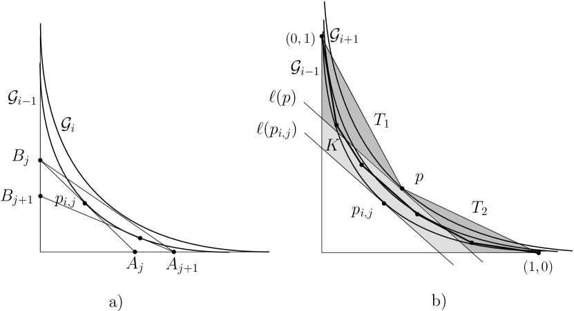
Figure 5. Long chains reaching above $\Gamma$

Next we define $\mathcal{G}_{i}^{*}$ ($i=0,1,\dots,f-1$) to be the event that there is a long convex chain $Y\subset X_{n}$ such that $\mathcal{G}_{i+1}$ is above $C(Y)$ but $\mathcal{G}_{i}$ is not above $C(Y)$, $i=0,1,\dots,f-1$. Further, let $\mathcal{G}_{i,j}^{*}$ be the event there is a long convex chain $Y\subset X_{n}$ with $C(Y)$ below $\mathcal{G}_{i+1}$ but not below $\ell(p_{i,j})$ (remember that $p_{i,j}\in\mathcal{G}_{i-1}$). Here $i=0,\dots,f-1$ and $j=1,\dots,\mathcal{J}(i)$. We have now the following result, similar to Lemma 8.3.

Lemma 8.5.

For every $i=0,\dots,f-1$ and every $j=1,\dots\mathcal{J}(i)$, $\mathbb{P}(\mathcal{G}_{i,j}^{*})\leq 3n^{-8\gamma^{2}/7}$.

This lemma immediately implies the following corollary.

Corollary 8.2.

The probability that there is a long convex chain $Y\subset X_{n}$ such that $C(Y)$ is not below $\Gamma_{\rho}$ is at most $3n^{-\gamma^{2}/7}$.

The proof follows from the facts that $\mathcal{G}_{i}^{*}\subset\bigcup_{j\in\mathcal{J}(i)}\mathcal{G}_{i,j}^{*}$, $f\leq n^{1/2}$, $\mathcal{J}(i)\leq n^{1/2}$, and $\gamma\geq 1$. Now we give the proof of Lemma 8.3 which is analogous to that of Lemma 8.3.

Proof of Lemma 8.5..

Let $\ell(p)$ be the unique tangent to $G_{i+1}$ which is parallel with $\ell(p_{i,j})$, and $p$ be the common point of $\ell(p)$ and $\Gamma_{i+1}$, see Figure 5 b). Let $T_{1},T_{2}$ be the two triangles determined by $p$ and $\ell(p)$, and let $K=K_{i,j}$ be the part of $T$ that lies between $\ell(p_{i,j})$ and $\ell(p)$. Since the distance of these two lines is at most $2\delta/\sqrt{8}$, $A(K)\leq\delta$.

A long convex chain $Y\subset X_{n}$ which is below $\mathcal{G}_{i+1}$ but not below $\ell(p_{i,j})$ splits into 3 parts: $Y_{1}=T_{1}\cap Y$, $Y_{2}=T_{2}\cap Y$, and $Y_{3}=K\cap Y$. Here $Y_{1},Y_{2}$ are convex chains in $T_{1}$ (from $(0,1)$ to $p$) and in $T_{2}$ (from $p$ to $(1,0)$), and $Y_{3}$ is in convex position in $K$. So

$$|Y_{1}|\leq L^{1},\;|Y_{2}|\leq L^{2},\mbox{ and }|Y_{3}|\leq M(K,n).$$

Since $Y$ is a long convex chain, $|Y_{1}|+|Y_{2}|+|Y_{3}|\geq|Y|\geq\mathbb{E}L_{n}-b$, and so $L^{1}+L^{2}+M(K,n)\geq\mathbb{E}L_{n}-b$. We are going to show that this event has small probability.

We apply Lemma 7.2 again with $\mu=b/5$. For sufficiently large $n$ the condition $1920\,e^{2}\,A(K)n\leq(b/5)^{3}$ is satisfied, since $A(K)\leq\delta=n^{-1/2}\sqrt{\log n}$ and $(b/5)^{3}=\gamma^{3}n^{1/2}(\log n)^{3/2}/125$. So we have, just as in (8.3),

$$\mathbb{P}(M(K,n)\geq b/5)<n^{-8\gamma^{2}/7}.$$

Therefore the estimate (8) applies without change:

$$\mathbb{P}(L^{1}+L^{2}+M(K,n)\geq\mathbb{E}L_{n}-b)\leq\mathbb{P}(L^{1}+L^{2}\geq\mathbb{E}L_{n}-1.2\,b)+n^{-8\gamma^{2}/7}.$$

Now Lemma 7.3 implies that $\mathbb{E}L^{1}+\mathbb{E}L^{2}\leq\mathbb{E}L_{n}-0.52R_{i+1}^{2}\sqrt[3]{n}$, and just as in (8),

$$\mathbb{P}(L^{1}+L^{2}\geq\mathbb{E}L_{n}-1.2\,b) \leq\sum_{i=1,2}\mathbb{P}(L^{i}\geq\mathbb{E}L^{i}+0.26R_{i+1}^{2}\sqrt[3]{n}-0.6\,b)$$

$$\leq\sum_{i=1,2}\mathbb{P}(L^{i}\geq\mathbb{E}L^{i}+4b).$$

Here the last step is justified just as in (8) except that this time $R_{i+1}\geq R_{1}=\rho+\delta$. Finally, we bound $\mathbb{P}(L^{i}\geq\mathbb{E}L^{i}+4b)$ the same way as in the proof of Lemma 8.3 to obtain

$$\mathbb{P}(L^{i}\geq\mathbb{E}L^{i}+4b)\leq n^{-8\gamma^{2}/7}.\qed$$

Proof of Theorem 1.3..

Considering Proposition 7.1, we have to estimate the probability that there is a longest convex chain not lying between $\Gamma_{-\rho}$ and $\Gamma_{\rho}$. This event splits into two parts: either the longest convex chain is not long, or there is a long convex chain not between $\Gamma_{-\rho}$ and $\Gamma_{\rho}$. The probability of the first event is estimated by Theorem 1.2, while the second part is handled via Corollaries 8.1 and 8.2. Therefore the probability in question is at most

$$n^{-\gamma^{2}/14}+n^{-\gamma^{2}/6}+6n^{-\gamma^{2}/7}<2n^{-\gamma^{2}/14}.\qed$$

Remarks. In this proof one can avoid using the estimate on $M(K,\mu)$. In fact, choosing $\delta$ and $\triangle$ small enough, the set $K$ contains more than $b/5$ points of $X_{n}$ with very small probability. So, with high probability, it cannot add much to the size of a long convex chain. There are more events $G_{i}^{*}$ and $G_{i,j}^{*}$, which has a minor effect on the final result. Also, the triangle $S$ in Lemma 8.1 is to be chosen much smaller.

An important step in our proof is Lemma 7.3, essentially implying that if the distance between $\Gamma$ and the farthest point of a convex chain from $\Gamma$ is “large”, then the chain cannot be too long. Conditioning on the location of this farthest point would allow an elegant conditional expectation argument. However, fixing the farthest point modifies the underlying probability space and therefore the estimate coming from Lemma 7.3 is no longer valid. To eliminate this difficulty, we chose to define finitely many subcases and estimate them separately, which can also be considered as a finite approximation of the continuous conditional expectation.

9. Numerical experiments

In the final section we summarize the observations obtained by computer simulations.

The search for the longest convex chains can be accomplished by an algorithm which has running time $O(n^{2})$. This algorithm works as follows. We order the points by increasing $x$ coordinate, and then recursively create a list at each point. The $k$th element on the list at point $p$ contains the minimal slope of the last segment of chains starting at $p_{0}$ and ending at $p$ whose length is exactly $k$, and a pointer to the other endpoint of this last segment. For creating the list at the next point $p$, we have to search the points before $p$, and see if $p$ can be added to the chains while preserving convexity.

This algorithm can be speeded up with some (not fully justified but useful) tricks. First of all, Theorem 1.3 guarantees that we have to search only among the points close to $\Gamma$. The simulations show that most longest convex chains are located in a small neighbourhood of $\Gamma$, whose radius is in fact of order approximately $n^{-1/3}$, much smaller than the width of order $n^{-1/12}$ given by Theorem 1.3. Therefore the search can be restricted to a subset of the points with cardinality of order $n^{2/3}$. Second, when looking for the longest chain, we have to search only points relatively close to $p$, and chains which are already relatively long, thus reducing memory demands.

$n$	$n^{-1/3}\mathbb{E}L_{n}$	$d_{n}$	Distance$/\sqrt{2}$	Deviation
1000	2.532	4	0.270	1.254
10000	2.768	5	0.200	1.383
15625	2.813	5	0.150	1.293
50000	2.885	5	0.100	1.411
75000	2.906	5	0.070	1.580
100000	2.917	5	0.060	1.431
125000	2.926	5	0.050	1.637
421875	2.959	5	0.012	1.732
1000000	2.976	6	0.012	2.023

Table 1. Results obtained by the simulation

With the above method, the search can be executed for up to $5\cdot 10^{4}$ active points, in which case examining one sample takes about 2 minutes. As the experiments show, this provides a good approximation for $n$’s up to order $10^{6}$. In each experiment, we increased the width of the searched neighbourhood until the increment did not generate a significant change in the average length of the longest convex chain. The results obtained by this method, although giving only a lower bound for $\mathbb{E}L_{n}$, are heuristically close to it. $\alpha=3$.

Figure 6. Results for $n^{-1/3}\mathbb{E}L_{n}$, illustrated as a function of $n^{1/3}$.

Our largest search has been done for $n=10^{6}$. The number of samples was $250$ except for the cases $n=25^{3}$ and $n=10^{6}$, where we used $500$ samples in order to model the distribution of $L_{n}$ (see Figure 7).

The results below well illustrate what the proof of Theorem 1.1 suggests, namely, that $n^{-1/3}\mathbb{E}L_{n}$ is increasing with $n$. Also, the data seem to confirm that $\alpha=3$.

Figure 7. Distribution of $L_{n}$, 500 samples, $n=25^{3}$ and $n=10^{6}$.

On Table 1 we list the results obtained by the program. The first column is the number of points chosen in $T$, the second is the average of $n^{-1/3}L_{n}$. The third column contains the half-length of the interval of the values of $L_{n}$, that is, $d_{n}=\lfloor\max|L_{n}-\mathbb{E}L_{n}|\rfloor$. This is noticeably small even for $n=10^{6}$. In the fourth column we list $1/\sqrt{2}$ times the radius of the neighbourhood of parabola we used for the search (the term $\sqrt{2}$ comes from a transformation of coordinates). The last data are the standard deviation of the set of values of $L_{n}$, ie. the square-root of its variance.

Figure 6 illustrates the linear interpolation of $n^{-1/3}\mathbb{E}L_{n}$ as a function of $n^{1/3}$. It is based on the data shown on Table 1.

As we know from Theorem 1.2, $L_{n}$ is highly concentrated near its expectation. This phenomenon is well recognizable on Figure 7, where we plot the distribution in the cases $n=25^{3}(=15625)$ and $n=10^{6}$ with $500$ samples.

10. Acknowledgements

We express our special thanks to Gábor Tusnády for his constant attention and interest in this piece of work, for valuable ideas concerning computer simulations, and in particular for pointing out an error in the earlier version of this paper. We also thank Zoltán Kovács for his suggestions regarding the implementation of the program. The second author was supported by Hungarian National Foundation Grants T 60427 and T 62321. Finally, we dedicate this piece of work to the memory of the late Professor Sándor Csörgő, whose zest for life and enthusiasm for mathematics will always be a constant inspiration to us.

References

[1] D. Aldous, P. Diaconis, Longest increasing subsequences:
from patience sorting to the Baik-Deift-Johansson theorem.
Bull. Amer. Math. Soc. 36 (1999), 413–432.
[2] N. Alon, J. Spencer, The probabilistic method. 2nd ed. John Wiley & Sons, New York, 2000.
[3] I. Bárány, Sylvester’s question: the probability
that points are in convex position. Ann. Probab. 27
(1999), no. 4., 2020–2034.
[4] I. Bárány, G. Rote, W. Steiger, C.-H. Zhang, A central
limit theorem for convex chains in the square. Discrete Comput.
Geom. 23 (2000), 35–50.
[5] I. Bárány, M. Prodromou, On maximal convex lattice
polygons inscribed in a plane convex set. Israel J. Math.
154 (2006), 337–360.
[6] W. Blaschke, Vorlesungen Über Differenzialgeometrie II. Affine Differenzialgeometrie.
Springer, Berlin, 1923.
[7] N. Enriquez, Convex chains in . To appear. Preprint
available online at http://arxiv.org/abs/math.PR/0612770
[8] B.F. Logan and L.A. Shepp, A variational problem for random Young tableaux.
Adv. Math. 26 (1977), 206–222.
[9] A. Rényi, R. Sulanke, Über die konvexe Hülle von zufällig gewählten Punkten. Z.
Wahrsch. Verw. Gebiete 2 (1963), 75–84.
[10] M. Talagrand, A new look at independence. Ann. Probab. 24
(1996), 1–34.
[11] P. Valtr, The probability that points are in convex position.
Discrete Comput. Geom. 13 (1995), 637–643.
[12] A.M. Vershik and S.V. Kerov,Asymptotics of the Plancherel measure
of the symmetric group and the limiting form of Young tables.
Dokl. Acad. Nauk. SSSR, 233 (1977), 1024–1027.
Gergely Ambrus
Department of Mathematics
University College London
Gower Street, London WC1E 6BT
England, U.K.
and
Bolyai Institute
University of Szeged
Aradi vért. tere 1, 6720 Szeged
Hungary
e-mail: g.ambrus@ucl.ac.uk
Imre Bárány
Rényi Institute of Mathematics
Hungarian Academy of Sciences
PO Box 127, 1364 Budapest
Hungary
and
Department of Mathematics
University College London
Gower Street, London WC1E 6BT
England, U.K.
e-mail: barany@renyi.hu