Sounding stellar cycles with Kepler – I. Strategy for selecting targets

Abstract

The long-term monitoring and high photometric precision of the Kepler satellite will provide a unique opportunity to sound the stellar cycles of many solar-type stars using asteroseismology. This can be achieved by studying periodic changes in the amplitudes and frequencies of the oscillation modes observed in these stars. By comparing these measurements with conventional ground-based chromospheric activity indices, we can improve our understanding of the relationship between chromospheric changes and those taking place deep in the interior throughout the stellar activity cycle. In addition, asteroseismic measurements of the convection zone depth and differential rotation may help us determine whether stellar cycles are driven at the top or at the base of the convection zone. In this paper, we analyze the precision that will be possible using Kepler to measure stellar cycles, convection zone depths, and differential rotation. Based on this analysis, we describe a strategy for selecting specific targets to be observed by the Kepler Asteroseismic Investigation for the full length of the mission, to optimize their suitability for probing stellar cycles in a wide variety of solar-type stars.

1 Introduction

Despite the enormous efforts that have been carried out over the past 400 years to observe and understand the solar cycle, the delayed onset of cycle 24 suggests that we still lack a complete understanding of this phenomenon (Zimmerman, 2009). One of the best ways to improve our understanding may be to study activity cycles in other stars, to help us understand stellar cycles in general and not just the solar cycle. Asteroseismology is emerging as one of the best tools available for the study of stellar cycles.

Astronomers have been making telescopic observations of sunspots since the time of Galileo, gradually building a historical record showing a periodic rise and fall in the number of sunspots every 11 years. We now know that sunspots are regions with an enhanced local magnetic field, so this 11-year cycle actually traces a variation in surface magnetism. Attempts to understand this behavior theoretically often invoke a combination of differential rotation, convection, and meridional flow to modulate the field through a magnetic dynamo (e.g., Dikpati & Gilman, 2006).

Significant progress in dynamo modeling could only occur after helioseismology provided meaningful constraints on the Sun’s interior structure and dynamics (Brown et al., 1989; Schou et al., 1998). Generally the models assume that the driving of the solar dynamo is related to large gradients in the rotation rate of different layers of the Sun, presumably those layers with the largest gradients, i.e. at the top and bottom of the near surface convection zone (Brandenburg, 2005).

Stellar activity has been monitored in more than 100 stars over the last 40 years with the Mount Wilson survey (Wilson, 1978; Baliunas & Vaughan, 1985; Baliunas et al., 1995). This survey has revealed that around half of the solar-type stars show clear periodic cycles, with periods between 2.5 and 25 years (Baliunas et al., 1995). Later studies of this and other samples such as the Lowell Observatory survey (Hall et al., 2007) suggest that there are two different branches of stellar cycles in solar-type stars – one active and one inactive (Saar & Brandenburg, 1999). This bifurcation, which is also known from the Vaughan-Preston gap (Vaughan & Preston, 1980) between active stars younger than 2.5 Gyr and older less active stars, can also be seen in the lengths of the stellar cycles as a function of the rotation period. Böhm-Vitense (2007) suggested, based on the fact that the number of rotations during a cycle seems to be different between the two subgroups of stars, that the bifurcation is caused by different dynamos operating in the two branches. Active stars generally have around 300 rotations per cycle, whereas inactive stars have around 100 rotations per cycle. According to Böhm-Vitense (2007), this suggests that stellar cycles in active stars are generated by the gradient in the rotation rate close to the surface, whereas the stellar cycles in inactive stars are generated by the gradient in the rotation rate at the base of the convection zone. In this scenario, a star with a given mass will start its life on the main sequence as a fast rotating active star with a relatively thin convection zone (Böhm-Vitense, 2007). Since the convective turnover time in stars with thinner convection zones is relatively short, these stars will have the largest rotational gradients near the surface, which would thus be where the dynamo would be driven in the stars on the active sequence. As the star evolves to the inactive sequence its surface rotation rate decreases significantly, which might be caused by additional deep mixing in a growing convection zone (Böhm-Vitense, 2007). This would result in the rotational gradient at the base of the convection zone growing larger than the rotational gradient near the surface, and therefore the dynamo would be driven at the base of the convection zone in the inactive stars. The larger rotational gradient would also require fewer rotations for the dynamo to create a toroidal magnetic field strong enough to rise to the surface.

Unfortunately, the Sun in many ways seems to fall between the two sequences of active and inactive stars – especially if one looks at the length of the stellar cycle as a function of the rotation period (Böhm-Vitense, 2007). This suggests that the Sun is not a good place to study stellar cycles, because two different dynamos might be operating in the Sun at the same time, confusing the picture. In other words, since the Sun seems to be in the transition from the active to the inactive sequence, it might be experiencing two different dynamos; one operating at the base of the convection zone and one operating at the top – as opposed to most other solar-type stars which are only experiencing one of the two dynamos. Evidence of this scenario can also be found in the discussion of whether the solar dynamo operates at the base or at the top of the convection zone (Brandenburg, 2005).

If we are to improve our understanding of the solar cycle, it seems that we need to study stellar cycles. To evaluate the different dynamo models, we need asteroseismic measurements to complement the activity measurements of stellar cycles – both in the sense of asteroseismic measurements of cycle-induced changes in the oscillation mode frequencies and amplitudes, and in the sense of asteroseismic measurements of the convection zone depth and differential rotation. The problem is that the stars in the Mount Wilson survey are relatively faint ($V\sim$ 6; Baliunas et al., 1995), making them unfit for dedicated ground-based asteroseismic networks like SONG (Grundahl et al., 2008), which are needed to obtain the extremely high frequency precision required for the analysis. The reason for this is of course that bright $G$ and $K$ stars are rare in the sky, the few exceptions are: $\alpha$ Cen A & B ($V$ = –0.01 and 1.33, respectively), 70 Oph A ($V$ = 4.03), $\kappa^{1}$ Cet ($V$ = 4.83) and the solar twin 18 Sco ($V$ = 5.5). It is therefore clear that the Kepler mission offers a unique possibility for sounding stellar cycles.

Once we have obtained a firm understanding of the solar cycle, we might be able to use the fact that the Sun seems to have a more complicated dynamo than most other solar-type stars as an advantage – as this may enable us to test more complicated dynamo models on the Sun. But the prolonged delay in the onset of cycle 24 has clearly shown us that we do not have a firm understanding of the solar cycle (Zimmerman, 2009).

This paper is the first in a series dedicated to the Kepler mission’s study of stellar cycles in solar-type stars. The paper evaluates the expected frequency precision for Kepler, the changes in the behavior of the stellar cycles on the main sequence and the effect of the convection zone depth and differential rotation on the acoustic spectra. Although the analysis in this paper is dedicated to the Kepler mission, it can also serve as a guide for selecting targets for other asteroseismic surveys, such as SONG.

We continue the analysis of the potential for sounding activity cycles in solar-type stars by Chaplin et al. (2007), but we now have the possibility to use specific estimates of the frequency precision for the Kepler mission. We also discuss problems with the way that the acoustic amplitude of the stellar cycles was estimated by Chaplin et al. (2007). The analysis of the signature of stellar rotation in the acoustic spectrum follows Chaplin et al. (2008a), but here we extend the analysis to include (1) updated estimates of mode lifetimes and the effect of these on the possibility of detecting the small rotational frequency splittings, and (2) the effect of differential rotation. Part of the analysis in this paper was done within asteroFLAG hare-and-hounds exercises as part of the preparation for the Kepler mission (Chaplin et al., 2008b) and some of the new scaling relations presented in this paper have thus been obtained from and tested on the artificial stars generated as part of the AsteroFLAG hare-and-hounds exercises.

The layout of the rest of the paper is as follows. In section 2 we review the details of the study of solar-type stars under the Kepler Asteroseismic Investigation (KAI). A review of the planned ground-based support for the study of stellar cycles in solar-type stars under the KAI is given in section 3 and an analysis of the expected frequency precision is given in section 4. Sections 5–7 use a number of isochrone tracks to estimate the effect of rotation (section 5), stellar cycles (section 6) and the convection zone (section 7) on the oscillation mode frequencies that we expect to measure from the observations. This analysis is used in a discussion of the best strategy for selecting the optimal full-length of the mission Kepler targets to increase our understanding of stellar cycles (section 8). Concluding remarks are found in section 9.

2 Kepler observations

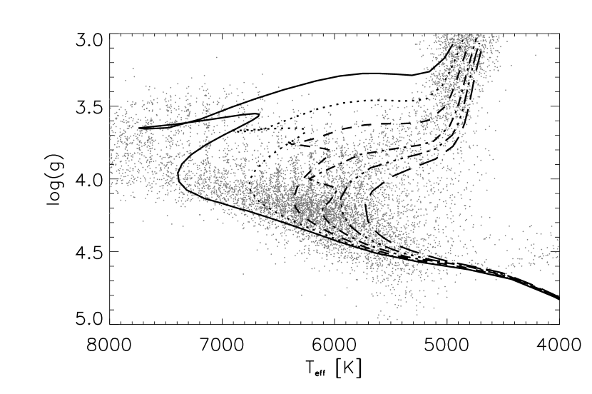
Figure 1: Padova isochrone tracks used in the analysis, shown as a function of effective temperature and surface gravity. The different line styles give the age of the stars: the solid line represents stars that are 1.0 Gyr old, dotted 1.6 Gyr, dashed 2.5 Gyr, dot-dashed 4.0 Gyr, dot-dot-dot-dashed 6.3 Gyr and long dashed 10.0 Gyr. This notation is used for the rest of the paper. The gray dots are stars from the Kepler Input Catalog with $g$-band magnitudes between 8 and 10.

Kepler is a NASA Discovery class space mission that was launched into an Earth trailing orbit on 7 March 2009, with the primary goal of detecting terrestrial planets using the transit method (Basri et al., 2005). The planned mission lifetime of Kepler is 42 months (excluding commissioning) with an optional extension of 30 months. The satellite is expected to be operational beyond the extended mission, but the downlink capability will be limited due to the distance between the satellite and the Earth. Kepler will monitor over 100,000 stars with a cadence of 30 min. In parallel with the planet program, Kepler also has an Asteroseismic Investigation (KAI; Christensen-Dalsgaard et al., 2007).

The KAI will begin with an initial run of 8 – 10 months depending on the length of the commission phase. In this survey phase of the mission, targets will only be observed for one month each. In the survey phase, close to 40,000 pixels are available for the KAI in short cadence (60 s). After the survey phase the KAI will shift to a specific target phase for the rest of the mission, and it is among these targets that it will be possible to study stellar cycles. In the specific target phase, the KAI will have the possibility to allocate 11,800 pixels for observations in short cadence. A conservative estimate is that around 3,000 of these 11,800 pixels will be allocated to $F$, $G$, and $K$ stars on the main sequence suitable for studying stellar cycles. The reason for giving these numbers in pixels and not as a quantity of targets is that bright stars will require more pixels than faint stars due to saturation. It is estimated that a 6th magnitude star will require 2,640 pixels, whereas a 12th magnitude star will only need 70 pixels. In practice, this means that the specific targets for studying stellar cycles could be chosen as e.g.: one 6th magnitude, ten 8th magnitude or 43 13th magnitude stars. The numbers of pixels that need to be allocated for stars at a given brightness are likely to decrease after the survey phase, when the characteristics of the instrument are better known. Kepler is designed to provide nearly photon noise limited photometry on saturated stars. The concept of doing photometry on saturated stars has been demonstrated with HST observations (Gilliland, 2008).

The targets for the survey phase have been chosen from the Kepler Input Catalog (Latham et al., 2005), and specific targets to be observed for the full-length of the mission must be chosen from the targets in the survey. It is expected that only observations from the first three months with be available before the specific targets need to be chosen, so in practice only targets from the first three months of observations can be selected as specific full-length of the mission targets. Fig. 1 shows all of the stars in the Kepler Input Catalog with $g$-band magnitude between 8 and 10, with Padova isochrone tracks (Bonatto et al., 2004; Girardi et al., 2002, 2004) plotted on top as a function of effective temperature and surface gravity. The isochrone tracks were calculated for 6 different ages between 1 and 10 Gyr in steps of 0.2 dex, using a metallicity of $z$ = 0.02. The same stars are plotted in Fig. 2, but here the targets selected for observations in the first three months of the survey phase are marked. It is seen that $F$ stars are highly over-represented compared to cooler stars in the first three months of the survey phase and in general. Although this reflects the stellar populations at a given magnitude bin, it is unfortunate as $F$ stars are the ones that are hardest to analyze with asteroseismology since they do not obey the asymptotic frequency relation (Tassoul, 1980) and have short mode lifetimes (Chaplin et al., 2009). The fraction of stars which show stellar cycles is also significantly larger among $G$ and $K$ stars than among $F$ stars (Baliunas et al., 1995).

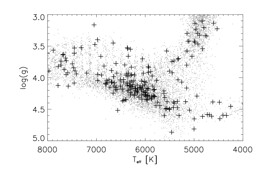
Figure 2: All stars in the Kepler Input Catalog with $g$-band magnitudes between 8 and 10 (gray dots) and targets chosen for observations in the first three months of the survey phase (black crosses).

3 Ground-based observations

Complementary ground-based chromospheric observations are important for mainly two reasons: firstly, they can be used to compare the cycle-induced changes in the chromosphere to changes in the amplitudes and frequencies of the oscillation modes – in other words, the complementary data provide a possibility to link the changes near the surfaces of the stars (i.e. in the chromospheres) to changes in the stellar interiors (i.e. in the oscillation modes). Secondly, ground-based chromospheric observations will be important if the cycles are significantly longer than the Kepler mission lifetime, or if the cycle-induced changes in the mode frequencies and amplitudes are too small to be measured with seismology. We will analyze the expected cycle lengths and seismic amplitudes in section 6.

We plan to measure the chromospheric activity of the coolest candidate targets discussed in section 2 during the summer of 2009 using the high-resolution FIbre-fed Echelle Spectrograph (FIES) mounted on the 2.6 meter Nordic Optical Telescope (Frandsen & Lindberg, 2000). After the specific targets have been selected, we will start to monitor the targets to look for stellar cycles in those stars. Note that even stars which show no sign of stellar cycles will be interesting, since it might be possible to use the asteroseismic measurement of the depths of the convection zones and rotation to understand why these stars show no sign of stellar cycles.

4 Expected frequency precision

Figure 3: Mode height as a function of effective temperature for the Padova isochrone tracks. It is seen that the mode height increases dramatically when the stars begin to evolve off the main sequence.

To estimate the potential for sounding stellar cycles, and for measuring the depths of the convection zones and differential rotation in the stars observed by Kepler, we first need to know what frequency precision we will be able to obtain from the observations. The frequency precision is determined by three parameters: the S/N of the oscillation modes in the acoustic spectrum, the mode lifetime $\tau$ and the length of the observations $T$ as given by the formulation of Libbrecht (1992):

$$\sigma_{\nu}=\sqrt{\frac{F(\beta)\Delta}{4\pi T}},$$ (1)

where $F(\beta)$ is a function of the inverse S/N, $\beta$:

$$F(\beta)=\sqrt{(1+\beta)}\left(\sqrt{(1+\beta)}+\sqrt{\beta}\right)^{3},$$ (2)

and $\Delta=1/(\pi\tau)$ is the mode FWHM linewidth. The Libbrecht formulation provides a lower limit on the frequency precision, since it does not account for blending effects in closely spaced oscillation modes. This is mainly a problem for modes with different azimuthal order, which is analyzed in detail in section 5.

We use the $T_{\rm eff}^{-4}$ scaling relation from Chaplin et al. (2009) for the mode lifetimes, which also provides us with the following relation for the height $H$ of the oscillation modes in the acoustic power density spectrum by using the scaling relation for the amplitude from Kjeldsen & Bedding (1995) for intensity observations:

$$H\propto g^{-2},$$ (3)

where $g$ is the surface gravity. Using the Padova isochrone tracks, we have plotted the mode height as a function of effective temperature in Fig. 3. It is seen that the mode height increases dramatically when the stars begin to evolve off the main sequence. It is also seen that the mode height decreases toward lower temperature, from 3 ${\rm ppm}^{2}/\mu{\rm Hz}$ for the Sun down to just over 1 ${\rm ppm}^{2}/\mu{\rm Hz}$ for stars with temperatures around 4500 K.

Figure 4: Frequency precision after 1 year of observations of a 9th magnitude star with Kepler as a function of effective temperature for the Padova isochrone tracks. The frequency precision scales with $1/\sqrt{T}$ where $T$ is the length of the observations. The frequency precision after 4 years of observations can therefore be calculated by dividing the numbers on the y-axis by 2.

Knowing the expected mode heights, we can use the expected photometric errors of the Kepler photometer to calculate the expected S/N. The photometric error is a function of many factors – the main one being the magnitude. It is estimated that the photometric error for a 60 sec integration $\sigma_{\rm int}$ with Kepler will be 45 ppm at 8th magnitude, 69 ppm at 9th magnitude and 111 ppm for a 10th magnitude star. The photometric errors are based on laboratory tests with fully flight-like electronics with an assumed level of stellar (activity and granulation) noise of 10 ppm (see Koch et al., 2000, for details of the laboratory tests). Assuming that the noise is random and uncorrelated, the photometric error can be converted into a power density error $\sigma_{\rm pd}$ using:

$$\sigma_{\rm pd}=2T_{\rm int}\sigma_{\rm int}^{2},$$ (4)

where $T_{\rm int}$ is the sampling time – i.e. 60 sec. In this way, we expect the error in the power density spectrum to be 0.24, 0.57 and 1.48 ${\rm ppm}^{2}/\mu{\rm Hz}$ for a 8th, 9th and 10th magnitude star, respectively. In comparison MOST, WIRE and CoRoT have obtained noise levels in the high-frequency part of the power density spectrum near the Nyquist frequency as low as 3, 1, and 0.15 ${\rm ppm}^{2}/\mu{\rm Hz}$, respectively (Guenther et al., 2008; Bruntt et al., 2005; Appourchaux et al., 2008). These values are not directly comparable to the expected error in the power density spectrum that we calculate for $Kepler$ since they are measured at high frequency and thus include very little activity and granulation signal, but it is clear that the expected error that we calculate does not seem unrealistic in comparison.

The estimated frequency precision for a 9th magnitude star as a function of effective temperature is shown in Fig. 4. It is seen that the evolved stars will yield the best frequency precision. It is also seen that the frequency precision improves toward lower effective temperature, from around the effective temperature of the Sun down to an effective temperature of 4500 K, but the slope is small. In other words, although the mode height changes on the main sequence, the frequency precision for oscillation modes in stars on the main sequence is approximately constant.

5 Prediction of rotation

Figure 5: Rotation frequency splitting as a function of effective temperature for the Padova isochrone tracks. It is seen that the rotational splitting decreases toward lower effective temperature.

The mean surface rotation period $P_{\rm rot}$ can be estimated from the empirical relationship given by Aigrain et al. (2004). This relationship is derived from photometric observations of stars in the Hyades (Radick et al., 1987, 1995). The relationship is:

$$\begin{array}[]{l}\mathrm{log}(P_{\rm rot})-0.5{\rm log}(t/0.625)=\\ \left\{\begin{array}[]{rll}-0.669+2.580(B-V)&{\rm for}&0.45\leq B-V\leq 0.62\\ 0.725+0.326(B-V)&{\rm for}&0.62<B-V\leq 1.30\end{array}\right.\end{array}$$ (5)

Here, $t$ is the age of the star in Gyr, and it appears in the relationship because the $t^{1/2}$ spin-down law of Skumanich (1972) is implicit.

When measuring stellar rotation with asteroseismology, it is the rotational frequency splitting $\Delta\nu_{\rm rot}$ that is measured rather than the rotation period. Assuming that the stars possess internal rotation rates that are comparable to the surface rates, as in the Sun, it is reasonable to assume that the mean rotation rate is given as the inverse of the mean rotation period. This might be questionable for younger stars (see Chaplin et al., 2008a, for discussion). As the oscillations that we are studying in this paper are high-order p modes we can also assume that the rotation frequency splittings equal the rotation rates. Note that this is not the case for, e.g. the high-order g modes in white dwarfs where the rotational splitting is only equal to half the rotation rate (Christensen-Dalsgaard, 2003). Under these assumptions the rotation period can easily be converted into an equivalent rotational frequency splitting by using the relation: $P_{\rm rot}=1/\Delta\nu_{\rm rot}$.

Fig. 5 shows the rotational frequency splitting as a function of effective temperature for the Padova isochrone tracks. It is generally seen that the rotational splitting deceases toward lower effective temperature and that the slope of this trend is much larger for stars hotter than the Sun compared to stars cooler than the Sun.

Figure 6: Ratio between rotational frequency splitting and the mode linewidth as a function of effective temperature for the Padova isochrone tracks. Note the interesting conclusion that the effective temperature of the Sun is the worst possible effective temperature at which rotational frequency splittings can be measured. This provides some hope that we will be able to measure differential rotation with asteroseismology.

5.1 Effect of finite mode lifetime

The possibility of measuring the rotational frequency splitting, and thus the mean rotation period of the stars, relies not only on a frequency precision sufficient to measure the small splittings, but also on splittings that are relatively large compared to the mode linewidth. If the linewidth is significantly larger than the splitting, it will not be possible to disentangle the modes of different azimuthal order $m$, and it will thus not be possible to measure the splittings. For this reason the internal rotation rate of the Sun was first obtained from low-degree helioseismology when it was realized that only low-frequency modes with long mode lifetime should be used for this analysis (Elsworth et al., 1995). Fig. 6 shows the ratio between the rotational frequency splittings and the mode linewidth, which can serve as a measure of the chances of disentangling the modes with different azimuthal order. The figure shows the surprising result that the effective temperature of the Sun is the worst possible effective temperature at which rotational frequency splittings can be measured.

As shown by García et al. (2004), it is just possible to measure radial differential rotation in the low-order frequency splittings from 6 years of low-degree observations of the Sun. Since the ratio between the rotational frequency splitting and the mode linewidth will be larger for all other stars on the main sequence, it is therefore not unreasonable to hope that we will be able to use Kepler to measure radial differential rotation in some solar-type stars with rotation profiles similar to the Sun.

In order to measure stellar rotation the rotation axis of the star needs to be inclined with respect to the line-of-sight. If the inclination angle between the rotation axis of the star and the line-of-sight is low, then the rotation will not significantly affect the frequencies of the observed oscillation modes with different azimuthal order, and the rotational frequency splitting can thus not be measured. Gizon & Solanki (2003) find that it is only possible to measure the rotational frequency splitting if the inclination angle is larger than around 30^∘. Statistically, assuming random orientation of the rotation axis, it will therefore not be possible to measure the rotational frequency splitting in around 15 per cent of the targets due to low inclination angles.

5.2 Effect of differential rotation

The Sun rotates fastest in the outer part of the convection zone beneath the equator, with a rotation rate of around 470 nHz. The rotation rate decreases to around 435 nHz at the base of the convection zone, and to around 450 nHz at the surface – with a further decrease along the surface to the poles with a value of around 370 nHz at 60^∘ which is the highest latitude at which rotation rates can be measured reliably with helioseismology (Schou et al., 1998). The largest gradients in the rotation rate are generally seen near the surface and near the base of the convection zone.

Differential rotation in the Sun and in other solar-type stars will manifest itself both as latitudinal and radial differential rotation. Latitudinal differential rotation is mainly on the surface, and can be measured either with asteroseismology or by fitting a spot model to the observed intensity time series as has been done for the stars $\kappa^{1}$ Ceti and $\epsilon$ Eri using the $MOST$ satellite (Croll et al., 2006; Walker et al., 2007). Radial differential rotation is confined to the stellar interior, and can only be measured with asteroseismology.

Differential rotation can be measured with asteroseismology by measuring differences in the separation between modes with different azimuthal order $m$ (the rotation splitting) over different radial orders $n$ and angular degrees $l$. A simplified way of doing this is by averaging the rotational splittings over different radial orders, and thus obtaining the splitting only as a function of the angular degree (see Gizon & Solanki, 2003, 2004; Ballot et al., 2006). This is done to increase the S/N of the measured splittings, but the approach in strongly biased towards measuring latitudinal differential rotation on the surface, and is much less efficient at measuring radial differential rotation at the base of the convection zone. For the Sun, the mean difference in the rotational splitting between $l=1$ and $l=2$ modes is around 7 nHz at low frequency (García et al., 2003). We therefore adopt this as a conservative reference value, although there might be better ways of averaging the rotational splittings for stars with thicker convection zones and thus larger radial rotation gradients (Böhm-Vitense, 2007). Such new averaging schemes would need to be calculated based on detailed forward modeling of the expected changes in the rotational splitting, not only over different angular degrees, but also over different radial orders. In this way, it would hopefully be possible to measure average rotational splittings that would be more sensitive to radial changes in the rotation rate at the base of the convection zone than to latitudinal changes in the rotation rate at the surface.

Figure 7: The difference in the rotational splitting between $l=1$ and $l=2$ modes averaged over different radial orders as a function of effective temperature for the Padova isochrone tracks. It is seen that the differences increase toward higher temperature and decrease with age.

Since only surface (latitudinal) differential rotation has been measured in other solar-type stars so far, we are only able to make predictions of the changes in the surface differential rotation on the main sequence. Surface differential rotation is normally expressed as the change in the rotation period $\Delta P_{\rm rot}$ over the stellar disc. A relation between $\Delta P_{\rm rot}$ and $P_{\rm rot}$ was obtained by Donahue et al. (1996) by looking at the changes in the rotation period measured in at least five different observing seasons in the stellar Ca ii measurements from Mount Wilson Observatory:

$$\Delta P_{\rm rot}\propto P_{\rm rot}^{1.3\pm 0.1}.$$ (6)

The interesting parameter for asteroseismology is not the change in the rotation period $\Delta P_{\rm rot}$ caused by differential rotation, but rather the change in the rotation rate $\Delta\Omega$. This can easily be obtained by assuming that $\Delta P_{\rm rot}\ll P_{\rm rot}$ and thus $\Delta\Omega\propto\Delta P_{\rm rot}/P_{\rm rot}^{2}$, which gives the following relation between the changes in the rotation rate caused by differential rotation and the mean rotation period:

$$\Delta\Omega\propto P_{\rm rot}^{-0.7\pm 0.1}.$$ (7)

Adopting 7 nHz as the mean difference in the rotational splitting between $l=1$ and $l=2$ modes at low frequency (García et al., 2003) in the Sun, we can plot the mean difference shown in Fig. 7. It is seen that the differences increase toward higher temperature and decrease with age.

The result in Fig. 7 should be seen as a lower limit on the effects of differential rotation that can be detected with asteroseismology, both because there might be better ways to measure radial differential rotation (as discussed above) and because differential rotation measured through changes in the rotation period samples a limited range of latitudes (see Donahue et al., 1996, for discussion).

Slightly higher values of the exponent in Eq. 6 have been found by Henry et al. (1995), who obtained an exponent of $1.76\pm 0.06$ based on photometry of active binaries, and Barnes et al. (2005) who obtained $1.85\pm 0.10$ based on Doppler imaging techniques and spectral analysis (Reiners & Schmitt, 2003). We have chosen to use the relation by Donahue et al. (1996) because the sample used in our study is not biased towards really active stars (as the photometry results) or towards really fast rotating stars (as the Doppler imaging and the spectral analysis results). The effect of increasing the exponent in Eq. 6 would be to flatten the curves in Fig. 7.

Differential rotation in solar-type stars has also been studied with mean-field models by Küker & Rüdiger (2008), who see a similar relation between $\Delta\Omega$ and the effective temperature as we see in Fig. 7 – i.e. the slope of the curves seems to increase dramatically at an effective temperature near 6000 K.

6 Prediction of stellar cycles

Figure 8: Stellar cycle period as a function of effective temperature for the Padova isochrone tracks. No general trend is seen.

A commonly used indicator of surface activity on stars is the Ca ii H and K emission index. This index is usually expressed as $R^{\prime}_{\rm HK}$ – the average fraction of the stellar luminosity that is emitted in the Ca ii H and K emission line cores (see Hall et al., 2007, for discussion). Using the first data from the Mount Wilson survey, Noyes et al. (1984) were able to obtain relations between the rotation period $P_{\rm rot}$, the $R^{\prime}_{\rm HK}$ index and the $B-V$ color, which can be used to obtain a scaling relation for the $R^{\prime}_{\rm HK}$ index:

$${\rm log}(\tau_{c}/P_{\rm rot})=-(0.324-0.400y+0.283y^{2}-1.325y^{3}),$$ (8)

where $y=$log$(R^{\prime}_{\rm HK}\times 10^{5})$ and $\tau_{c}$ is the convective turnover time. The convective turnover time may then be calculated from:

$$\begin{array}[]{l}{\rm log}(\tau_{c})=\\ \left\{\begin{array}[]{rrll}1.361+0.166x&+0.025x^{2}-5.323x^{3}&{\rm for}&x\geq 0\\ 1.361-0.140x&&{\rm for}&x<0\end{array}\right.\end{array}$$ (9)

where $x=1-(B-V)$ and the convective turnover time is measured in days. To calculate the $R^{\prime}_{\rm HK}$ index, we solve the cubic Eq. 8 using the known input parameters: $B-V$ and $P_{\rm rot}$.

Knowing the $R^{\prime}_{\rm HK}$ index, we can calculate the cycle period $P_{\rm cyc}$ from the relation given by Chaplin et al. (2008a):

$$\begin{array}[]{l}{\rm log}(P_{\rm cyc})=\\ \left\{\begin{array}[]{rll}-6.7-1.6{\rm log}(R^{\prime}_{\rm HK})&{\rm for}&{\rm log}(R^{\prime}_{\rm HK})<-4.75\\ -5.5-1.4{\rm log}(R^{\prime}_{\rm HK})&{\rm for}&{\rm log}(R^{\prime}_{\rm HK})\geq-4.75\\ \end{array}\right.\end{array}$$ (10)

Fig. 8 shows the expected stellar cycle period as a function of effective temperature. No general trend is seen. For the three youngest isochrones, it is seen that the cycle period generally increases toward higher temperature. For effective temperatures lower than the effective temperature of the Sun, it is seen that the cycle periods generally increase with age as the stars evolve from active to inactive stars while their rotation periods decrease. On the other hand, as the stars evolve from the active to the inactive sequence, the number of rotations in each stellar cycle decreases and therefore no general trend is seen in the figure.

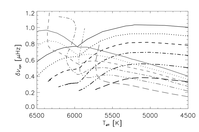
Figure 9: Stellar cycle frequency shifts as a function of the effective temperature for the Padova isochrone tracks. For the black lines the shifts were calculated using the scaling relation $\delta\nu_{\rm cyc}\propto\Delta R^{\prime}_{\rm HK}$ from Chaplin et al. (2007) and for the gray lines the shifts were calculated using the scaling relation $\delta\nu_{\rm cyc}\propto\frac{R^{2.5}L^{0.25}}{M^{2}}\Delta R^{\prime}_{\rm HK}$ from Metcalfe et al. (2007). It is seen that the shifts calculated using the scaling relation by Chaplin et al. (2007) are nearly constant for stars cooler than 5500 K, while at the same age the shifts calculated using the scaling relation by Metcalfe et al. (2007) generally decrease around 50 per cent between 5500 K and 4500 K.

The amplitudes of the activity cycles $\Delta R^{\prime}_{\rm HK}$ can be obtained from the relation given by Saar & Brandenburg (2002):

$$\Delta R^{\prime}_{\rm HK}\propto(R^{\prime}_{{\rm HK}})^{0.77}.$$ (11)

The p-mode frequencies in the Sun are generally believed to be affected by the solar cycle through changes in the turbulent velocity in the outermost regions of the near surface convection zone, caused by changes in the RMS magnetic field in the Sun (Dziembowski & Goode, 2004, 2005). Relations between the Ca ii amplitudes of the activity cycles $\Delta R^{\prime}_{\rm HK}$ and the cycle frequency shifts $\delta\nu_{\rm cyc}$ have been proposed by Chaplin et al. (2007) and Metcalfe et al. (2007).

Chaplin et al. (2007) proposed that the cycle frequency shifts simply scale linearly with the amplitudes of the activity cycles:

$$\delta\nu_{\rm cyc}\propto\Delta R^{\prime}_{\rm HK}.$$ (12)

Evidence for this relation is found from observations of low-degree oscillations in the Sun, where it is seen that the cycle frequency shifts change linearly with changes in the Mg ii lines over the solar cycle (Chaplin et al., 2007). The expected stellar cycle frequency shifts as a function of the effective temperature obtained using the scaling from Chaplin et al. (2007) is shown in Fig. 9 (black lines). It is seen that the cycle frequency shifts generally increase toward lower temperature and decrease with age.

On the other hand, Metcalfe et al. (2007) assume that the cycle frequency shifts scale as

$$\delta\nu_{\rm cyc}\propto\frac{D}{I}\Delta R^{\prime}_{\rm HK},$$ (13)

where $D$ is the depth of the source of the perturbations beneath the photosphere and $I$ is the mode inertia. The inverse relation with the mode inertia is known from studies of solar cycle mode frequency shifts (see Libbrecht & Woodard, 1990; Dziembowski & Goode, 2004, 2005, for discussion). Metcalfe et al. (2007) then assume that the mode inertia scales as $M/R$ and that the source depth scales with the pressure scale height at the photosphere $H_{p}$, which itself scales as $L^{0.25}R^{1.5}/M$. We thus obtain:

$$\delta\nu_{\rm cyc}\propto\frac{R^{2.5}L^{0.25}}{M^{2}}\Delta R^{\prime}_{\rm HK},$$ (14)

Note that we lack a physical argument for the relation between the source depth and the pressure scale height other than the fact that most things in the near surface layers scale with the pressure scale height. The Kepler observations might eventually provide us with such arguments as it might be possible to extract information of the location of the source of the p-mode excitation from the high-frequency oscillations in the solar-type stars as has been done for the Sun (Kumar & Lu, 1991) and other solar-type stars (Karoff, 2007), but it remains to be proven if similar kinds of analysis could also reveal the location of the source of the perturbations caused by the stellar cycles.

Fig. 9 also shows the expected stellar cycle frequency shifts as a function of the effective temperature obtained by using the scaling from Metcalfe et al. (2007) (gray lines). It is seen that the shifts generally increase toward higher temperature and decrease with age. The shifts calculated using the scaling relation by Chaplin et al. (2007) are nearly constant for stars cooler than 5500 K but with the same age. On the other hand, the shifts calculated using the scaling relation by Metcalfe et al. (2007) generally decrease around 50 per cent between 5500 K and 4500 K for a given age. It is currently not possible to determine which of the two scaling relations is more appropriate, but it is clear from Figs. 4 & 9 that we will be able to measure the oscillation mode frequencies precisely enough from one year of Kepler data to detect stellar cycle frequency shifts when these frequencies are compared to Kepler observations obtained in other years. We also note that the Kepler observations might allow us to test which of the scaling relations is the better one.

7 Prediction of the convection zone depth

One of the most important things that will help us understand the stellar cycles we observe with Kepler is a measurement of the convection zone depth. The depth of the convection zone can be measured with asteroseismology by analyzing the second differences in the frequencies:

$$\Delta_{2}\nu_{n,l}\equiv\nu_{n-1,l}-2\nu_{n,l}+\nu_{n+1,l}$$ (15)

Localized regions of rapid variation of the sound speed, such as the bottom of the convection zone, will induce an oscillatory component in the second frequency differences as a function of frequency (Monteiro et al., 2000; Houdek & Gough, 2007). Other localized regions that cause oscillatory components in the second frequency differences are the ionization zones of He i and He ii. Houdek & Gough (2007) have given full analytical solutions for how to represent the oscillatory components in the second frequency differences from the three regions. For the analysis here, we are only interested in determining how the amplitude of the oscillatory component originating from the base of the convection zone depends on fundamental stellar parameters.

To evaluate how the amplitude of the oscillatory component originating from the base of the convection zone changes with fundamental stellar parameters, we have used frequencies from 6 artificial solar-type stars generated as part of the asteroFLAG hare-and-hounds exercises (Chaplin et al., 2008b). The amplitudes of the oscillatory components in these stars were measured by calculating the least-squares periodogram of the second differences. These periodograms all showed 3 peaks from the 3 regions of rapid variation of the sound speed, and the peak with the highest frequency is the one that originates from the base of the convection zone. We then looked for correlations between the amplitude of the peak originating from the base of the convection zone and the effective temperature and surface gravity. It was seen that there was a clear correlation between the logarithm of the surface gravity ${\rm log}(g)$ and the amplitude of the form:

$$A_{\rm cz}\propto{\rm log}(g).$$ (16)

We adopt a value of 0.4 $\mu$Hz for the mean amplitude of the oscillatory component in the second frequency differences in the Sun (Houdek & Gough, 2007). Fig. 10 shows the amplitude of the oscillatory component originating from the base of the convection zone as a function of the effective temperature. It is seen that the amplitude generally increases toward lower temperature.

Figure 10: The amplitude of the oscillatory component in the second frequency differences originating from the base of the convection zone as a function of the effective temperature for the Padova isochrone tracks.

Roxburgh (2009) has recently suggested another approach for measuring the convection zone depth with asteroseismology. This method makes use of the second and third frequency differences between modes of angular degree 0 and 1 instead of the second differences of modes with the same degree. This method has the advantage that the amplitude of the oscillatory component of the differences is constant as a function of frequency – whereas it decreases toward higher frequencies for the differences from modes with the same degree. Also, the method can be tuned so that the signal from the He ii ionization zone cancels out, which makes it easier to detect the signal from the base of the convection zone. However, the method has two weaknesses compared to the differences from modes with the same degree. Firstly, it only uses information from modes with degree 0 and 1, and not from modes with degree 2 that we will also detect in the Kepler observations (which means that not all information from the observations is used to measure the depth of the convection zone). Secondly, it is not clear whether the signal from the He ii ionization zone can be canceled out in stars other than the Sun.

The signal from the base of the convection zone in the method by Roxburgh (2009) will also scale with log($g$) as suggested in Eq. 16, though the absolute amplitude and S/N could be different from the amplitudes and S/N obtained for the second differences from modes with the same degree.

8 Discussion

Below we summarize the different recommendations for selecting asteroseismic targets for sounding stellar cycles.

8.1 Effect of stellar brightness and S/N of observations

At 8th magnitude the S/N of the oscillation modes will allow the detection of modes in all stars, and the frequency precision will mainly be limited by (1) the mode lifetime, which will cause the power to be smeared out over a larger frequency range, and (2) the length of the observations. 9th magnitude stars will allow the detection of oscillations in most cases. Here the frequency precision for stars with long mode lifetimes will be limited not only by the mode lifetime and the length of the observations, but also by the S/N. 10th magnitude stars will only allow the detection of oscillation modes for temperatures similar to the Sun and hotter, and the frequency precision will be limited by the S/N for most mode lifetimes.

8.2 Optimal stellar parameters for measuring stellar rotation with asteroseismology

The worst place in parameter space for measuring stellar rotation with asteroseismology is the place of the Sun – both hotter and cooler stars will have larger rotational splittings relative to the mode linewidths in the acoustic spectrum. Differential rotation will generally be measured most easily in young stars. For stars hotter than 6000 K, differential rotation will be measured most easily in the hottest stars, while there is almost no dependence on temperature for stars cooler than 6000 K.

8.3 Optimal stellar parameters for activity cycles

The analysis did not provide a clear answer to where on the main sequence it will be easiest to sound stellar cycles. It is clear that young stars will generally have shorter periods and larger frequency changes caused by stellar cycles. In order to use asteroseismology to investigate the hypothesis put forward by Böhm-Vitense (2007) – that the Vaughan-Preston gap is caused by two different kinds of dynamos operating on either side of the gap — it is important that stars on either side of the gap are observed with Kepler. The best way to determine which side of the gap the stars are on is by determining their ages (see section 8.6).

8.4 Optimal stellar parameters for measuring the convection zone depth

It will generally be easier to measure the depth of the stellar convection zone in cooler stars, since the amplitudes in the second frequency differences are expected to be larger than in hotter stars. The analysis has shown that we can expect to measure the convection zone depth in all KAI full length of the mission specific targets in the analyzed range in effective temperature.

8.5 General optimal stellar parameters for sounding stellar cycles

From these recommendations it is generally seen that the targets should be as young as possible, with the reservation that both sides of the Vaughan-Preston gap need to be sampled.

The analysis of the effect of differential rotation and stellar cycles on the acoustic spectra favors hotter stars, though the dependence is not strong and unambiguous. The effect of the convection zone depth favors cooler stars. We thus conclude that stars both cooler and hotter than the Sun should be on the KAI full length of the mission specific targets list, and to ensure a relatively equal distribution this means that we should favor cooler stars since they are clearly under-abundant among the targets already selected for observations in the first three months of the survey phase.

It is clear that measuring stellar differential rotation will be the most demanding task of those analyzed here, and this task will set high demands on the frequency precision. This means that it will only be possible to measure stellar differential rotation with asteroseismology on Kepler stars after they have been observed for the full length of the mission. On the other hand, the analysis has shown that evaluating the potential for measuring stellar differential rotation based on the frequency shifts seen in the Sun from differential rotation is probably too pessimistic. This provides some hope that we will be able to measure stellar differential rotation in some of the stars observed with Kepler.

The analysis has also shown that it is probably going to be possible to measure the oscillation mode frequencies precisely enough in one year of Kepler data to be able to see stellar cycle frequency shifts when these frequencies are compared to Kepler observations obtained in other years. It also seems possible to measure the depth of the convection zone from just one year of Kepler observations, though the full data set will eventually be available for this purpose.

It is also worth noting that mode frequency shifts might not be the only way to sound the stellar cycles. The stellar cycles will also manifest themselves as changes in the amplitudes and lifetimes of the modes (Chaplin et al., 2000), and possibly also in flare induced high-frequency oscillations (Karoff & Kjeldsen, 2008), though the last concept remains to be proven.

8.6 Asteroseismic determination of stellar age

Since one of the recommendations is that mainly young stars should be selected, we need a way to determine the stellar ages. The best tool for doing this is asteroseismology, and it is reasonable to assume that a rough age estimate can be obtained from the survey observations by plotting the small and large frequency separations in the asteroseismic HR-diagram (also known as the JC-D diagram, Christensen-Dalsgaard et al., 2007). Since we are interested in stars around the Vaughan-Preston gap (age 2–3 Gyr), we can safely assume that the lines in the asteroseismic HR-diagram are vertical to within the precision needed for Kepler specific target selection. This basically means that we are mainly interested in stars which have a small separation equal to the small separation in the Sun (6 $\mu$Hz) and larger.

8.7 Recommendations for Kepler target selection for sounding stellar cycles

We finally end up with the following selection procedure:

1. Use the targets with magnitudes between 8 and 10 in the first 3 months of the Kepler survey phase as candidates.

2. Start selecting stars from the cool end.

3. Ensure that the oscillations can be seen in the acoustic spectrum.

4. Ensure that the oscillation modes can be understood in the framework of the asymptotic frequency relation.

5. Ensure that hints of rotational splitting can be seen.

6. Ensure that the small separation is large (6 $\mu$Hz).

7. Ensure that both active and inactive stars have been selected (based on ground-based observations of chromospheric activity in the stars).

9 Conclusions

We have presented an analysis of the potential for using observations from the Kepler Asteroseismic Investigation to improve our understanding of solar and stellar cycles. The analysis has shown that it will probably be possible to sound stellar cycles with Kepler in stars brighter than 9th magnitude by measuring the changes in the oscillation mode frequencies caused by the stellar cycles. It should be possible to measure the depth of the convection zone and the mean rotation rate from Kepler observations of stars brighter than 9th magnitude. The analysis has also revealed that measuring stellar differential rotation will be highly demanding on the frequency precision, and it is clear that it will only be possible after the mission has finished. On the other hand, one of the unexpected results of the analysis was that the worst place in parameter space for measuring stellar rotation with asteroseismology is the place of the Sun – which provides some hope that it might be possible to measure stellar differential rotation in some of the stars observed with Kepler.

The scaling relations we use for rotation, mode lifetime, activity etc. represent a statistical average of the behavior of many, or several, stars, observed by photometry, spectroscopy and asteroseismology. Provided these relations are accurate, our predictions are therefore those for a notional average field star. Natural scatter means that e.g. not all stars hotter or cooler than the Sun will present a smaller challenge when it comes to rotation; however, given a sufficient number of stars, we predict that on average, things will be easier.

References

- Aigrain et al. (2004) Aigrain, S., Favata, F., & Gilmore, G. 2004, A&A, 414, 1139
- Appourchaux et al. (2008) Appourchaux, T., et al. 2008, A&A, 488, 705
- Baliunas et al. (1995) Baliunas, S. L., et al. 1995, ApJ, 438, 269
- Baliunas & Vaughan (1985) Baliunas, S. L., & Vaughan, A. H. 1985, ARA&A, 23, 379
- Ballot et al. (2006) Ballot, J., García, R. A., & Lambert, P. 2006, MNRAS, 369, 1281
- Barnes et al. (2005) Barnes, J. R., Cameron, A. C., Donati, J.-F., James, D. J., Marsden, S. C., & Petit, P. 2005, MNRAS, 357, L1
- Basri et al. (2005) Basri, G., Borucki, W. J., & Koch, D. 2005, New Astronomy Review, 49, 478
- Bonatto et al. (2004) Bonatto, C., Bica, E., & Girardi, L. 2004, A&A, 415, 571
- Brandenburg (2005) Brandenburg, A. 2005, ApJ, 625, 539
- Brown et al. (1989) Brown, T. M., Christensen-Dalsgaard, J., Dziembowski, W. A., Goode, P., Gough, D. O., & Morrow, C. A. 1989, ApJ, 343, 526
- Bruntt et al. (2005) Bruntt, H., Kjeldsen, H., Buzasi, D. L., & Bedding, T. R. 2005, ApJ, 633, 440
- Böhm-Vitense (2007) Böhm-Vitense, E. 2007, ApJ, 657, 486
- Chaplin et al. (1999) Chaplin, W. J., et al. 1999, MNRAS, 308, 405
- Chaplin et al. (2000) Chaplin, W. J., Elsworth, Y., Isaak, G. R., Miller, B. A., & New, R. 2000, MNRAS, 313, 32
- Chaplin et al. (2007) Chaplin, W. J., Elsworth, Y., Houdek, G., & New, R. 2007, MNRAS, 377, 17
- Chaplin et al. (2007) Chaplin, W. J., Elsworth, Y., Miller, B. A., Verner, G. A., & New, R. 2007, ApJ, 659, 1749
- Chaplin et al. (2008a) Chaplin, W. J., Houdek, G., Appourchaux, T., Elsworth, Y., New, R., & Toutain, T. 2008a, A&A, 485, 813
- Chaplin et al. (2008b) Chaplin, W. J., et al. 2008b, Astronomische Nachrichten, 329, 549
- Chaplin et al. (2009) Chaplin, W. J., Houdek, G., Karoff, C., Elsworth, Y., & New, R. 2009, A&A, in press, (arXiv:0905.1722)
- Christensen-Dalsgaard (1984) Christensen-Dalsgaard, J. 1984, Space Research in Stellar Activity and Variability, 11
- Christensen-Dalsgaard (2003) Christensen-Dalsgaard, J. 2003, Lecture Notes on Stellar Oscillations, 5th ed. On-line at http://astro.phys.au.dk/jcd/oscilnotes/
- Christensen-Dalsgaard et al. (2007) Christensen-Dalsgaard, J., Arentoft, T., Brown, T. M., Gilliland, R. L., Kjeldsen, H., Borucki, W. J., & Koch, D. 2007, Communications in Asteroseismology, 150, 350
- Croll et al. (2006) Croll, B., et al. 2006, ApJ, 648, 607
- Dikpati & Gilman (2006) Dikpati, M., & Gilman, P. A. 2006, ApJ, 649, 498
- Donahue et al. (1996) Donahue, R. A., Saar, S. H., & Baliunas, S. L. 1996, ApJ, 466, 384
- Dziembowski & Goode (2004) Dziembowski, W. A., & Goode, P. R. 2004, ApJ, 600, 464
- Dziembowski & Goode (2005) Dziembowski, W. A., & Goode, P. R. 2005, ApJ, 625, 548
- Elsworth et al. (1995) Elsworth, Y., Howe, R., Isaak, G. R., McLeod, C. P., Miller, B. A., New, R., Wheeler, S. J., & Gough, D. O. 1995, Nature, 376, 669
- Frandsen & Lindberg (2000) Frandsen, S., & Lindberg, B. 2000, The Third MONS Workshop: Science Preparation and Target Selection, 163
- García et al. (2004) García, R. A., et al. 2004, Solar Phys., 220, 269
- García et al. (2003) García, R. A., Eff-Darwich, A., Korzennik, S. G., Couvidat, S., Henney, C. J., & Turck-Chièze, S. 2003, GONG+ 2002. Local and Global Helioseismology: the Present and Future, 517, 271
- García et al. (2008) García, R. A., Mathur, S., Ballot, J., Eff-Darwich, A., Jiménez-Reyes, S. J., & Korzennik, S. G. 2008, Solar Phys., 251, 119
- Gilliland (2008) Gilliland, R. L. 2008, AJ, 136, 566
- Girardi et al. (2002) Girardi, L., Bertelli, G., Bressan, A., Chiosi, C., Groenewegen, M. A. T., Marigo, P., Salasnich, B., & Weiss, A. 2002, A&A, 391, 195
- Girardi et al. (2004) Girardi, L., Grebel, E. K., Odenkirchen, M., & Chiosi, C. 2004, A&A, 422, 205
- Gizon & Solanki (2003) Gizon, L., & Solanki, S. K. 2003, ApJ, 589, 1009
- Gizon & Solanki (2004) Gizon, L., & Solanki, S. K. 2004, Sol. Phys., 220, 169
- Grundahl et al. (2008) Grundahl, F., Arentoft, T., Christensen-Dalsgaard, J., Frandsen, S., Kjeldsen, H., & Rasmussen, P. K. 2008, Journal of Physics Conference Series, 118, 01204
- Guenther et al. (2008) Guenther, D. B., et al. 2008, ApJ, 687, 1448
- Hall et al. (2007) Hall, J. C., Lockwood, G. W., & Skiff, B. A. 2007, AJ, 133, 862
- Henry et al. (1995) Henry, G. W., Eaton, J. A., Hamer, J., & Hall, D. S. 1995, ApJS, 97, 513
- Houdek & Gough (2007) Houdek, G., & Gough, D. O. 2007, MNRAS, 375, 86
- Karoff (2007) Karoff, C. 2007, MNRAS, 381, 1001
- Karoff & Kjeldsen (2008) Karoff, C., & Kjeldsen, H. 2008, ApJ, 678, L7
- Kjeldsen & Bedding (1995) Kjeldsen, H., & Bedding, T. R. 1995, A&A, 293, 87
- Koch et al. (2000) Koch, D. G., Borucki, W. J., Dunham, E. W., Jenkins, J. M., Webster, L., & Witteborn, F. 2000, SPIE, 4013, 508
- Kumar & Lu (1991) Kumar, P., & Lu, E. 1991, ApJ, 375, L35
- Küker & Rüdiger (2008) Küker, M., Rüdiger, G. 2008, Journal of Physics Conference Series, 118, 01202
- Latham et al. (2005) Latham, D. W., Brown, T. M., Monet, D. G., Everett, M., Esquerdo, G. A., & Hergenrother, C. W. 2005, Bulletin of the American Astronomical Society, 37, 1340
- Libbrecht (1992) Libbrecht, K. G. 1992, ApJ, 387, 712
- Libbrecht & Woodard (1990) Libbrecht, K. G., & Woodard, M. F. 1990, Nature, 345, 779
- Metcalfe et al. (2007) Metcalfe, T. S., Dziembowski, W. A., Judge, P. G., & Snow, M. 2007, MNRAS, 379, L16
- Monteiro et al. (2000) Monteiro, M. J. P. F. G., Christensen-Dalsgaard, J., & Thompson, M. J. 2000, MNRAS, 316, 165
- Noyes (1983) Noyes, R. W. 1983, Solar and Stellar Magnetic Fields: Origins and Coronal Effects, 102, 501
- Noyes et al. (1984) Noyes, R. W., Hartmann, L. W., Baliunas, S. L., Duncan, D. K., & Vaughan, A. H. 1984, ApJ, 279, 763
- Radick et al. (1987) Radick, R. R., Thompson, D. T., Lockwood, G. W., Duncan, D. K., & Baggett, W. E. 1987, ApJ, 321, 459
- Radick et al. (1995) Radick, R. R., Lockwood, G. W., Skiff, B. A., & Thompson, D. T. 1995, ApJ, 452, 332
- Reiners & Schmitt (2003) Reiners, A., & Schmitt, J. H. M. M. 2003, A&A, 398, 647
- Roxburgh (2009) Roxburgh, I. W. 2009, A&A, 493, 185
- Saar & Brandenburg (1999) Saar, S. H., & Brandenburg, A. 1999, ApJ, 524, 295
- Schou et al. (1998) Schou, J., et al. 1998, ApJ, 505, 390
- Skumanich (1972) Skumanich, A. 1972, ApJ, 171, 565
- Tassoul (1980) Tassoul, M. 1980, ApJSS, 43, 469
- Vaughan & Preston (1980) Vaughan, A. H., & Preston, G. W. 1980, PASP, 92, 38
- Walker et al. (2007) Walker, G. A. H., et al. 2007, ApJ, 659, 1611
- Wilson (1978) Wilson, O. C. 1978, ApJ, 226, 379
- Zimmerman (2009) Zimmerman, R. 2009, ScienceNOW Daily News, 8 May