Ginzburg-Landau theory of dirty two band $s_{\pm}$ superconductors

Abstract

In this paper we study the effect of non-magnetic impurities on two-band $s_{\pm}$ superconductors by deriving the corresponding Ginzburg-Landau (GL) equation. Depending on the strength of (impurity-induced) inter-band scattering we find that there are two distinctive regions where the superconductors behave very differently. In the strong impurity induced inter-band scattering regime $T_{c}<<\tau^{-1}_{t}$, where $\tau_{t}\sim$ mean-life time an electron stays in one band the two-band superconductor behaves as an effective one-band dirty superconductor. In the other limit $T_{c}\geq\tau^{-1}_{t}$, the dirty two-band superconductor is described by a network of frustrated two-band superconductor grains connected by Josepshon tunnelling junctions. We argue that most pnictide superconductors are in the later regime.

With the discovery of the Iron-based (pnictides) superconductors, superconductivity characterized by more than one order parameters, i.e. the multi-gap superconductors, becomes a topic of interests. Band structure calculations indicate that the materials have a quasi-two-dimensional electronic structure, with five bands centered around the $\Gamma$- and $M$- points in the Brillouin zone contributing to the Fermi surface. It has been proposed that the superconducting order parameters in this multi-band materials has so called $s_{\pm}$-wave symmetry, where the order parameters have $s$-symmetry but with opposite sign between bands centered at $\Gamma$- and $M$-pointshu ; mazin ; wang .

The effect of impurities in this class of materials has been an issue of interests. NMRNMR1 and lower critical field datafield seems to suggest the existence of nodes in the superconducting order parameter while APRES experiemntsARPES1 ; ARPES2 favor node-less gaps. One possible solution to this controversy is that large number of in gap states are induced by impurities in the material because of the special $s_{\pm}$ order-parameters. Indeed, such a scenario has received supports from self-consistent-Born type calculation where in gap states are found to appear easily in $s_{\pm}$ superconductorsim1 ; im2 .

In this paper we study the effect of non-magnetic impurities on two-band $s_{\pm}$-wave superconductors by analyzing the corresponding Ginzburg-Landau theory. The effect of impurities is included by generalizing the standard Bogoliubov de Gennes theoryBdG and diagrammatic perturbation techniquesplee which have been applied to study the effect of impurities on single-band superconductorsBdG ; whh ; kotliar to the case of two-band superconductors.

We start with the Bogoliubov-de Gennes formulation of BCS theoryBdG . The system we consider is characterized by a BCS Hamiltonian, $H=H_{0}+V_{BCS}$, where

$$H_{0}=\sum_{i,j,\sigma}\int d^{d}r\psi^{+}_{i\sigma}(\vec{r})\left(\delta_{ij}\hat{H}_{0i}(\nabla)+U_{ij}(\vec{r})\right)\psi_{j\sigma}(\vec{r})$$ (1a)

where $$i,j=1,2 \sigma=\uparrow,\downarrow H_{0i}(\nabla) i U_{ij}(\vec{r}) i=j i\neq j \psi_{j\sigma}(\psi^{+}_{j\sigma})$$ and are the band and spin indices, respectively. is the band Hamiltonian describing electronic wave-functions in band . is a non-magnetic disordered potential which scatters electrons both within () and between () bands. are electron annihilation (creation) operators.

$$V_{BCS}=-\sum_{i,j,\sigma}V_{ij}\int d^{d}r\psi^{+}_{i\sigma}(\vec{r})\psi^{+}_{i\bar{\sigma}}(\vec{r})\psi_{j\bar{\sigma}}(\vec{r})\psi_{j\sigma}(\vec{r}),$$ (1b)

is the BCS interaction between electrons, $\bar{\sigma}=-\sigma$. We note that $V_{ij}>0$ means attractive interaction in our notation. Introducing the BCS decoupling,

$$\psi^{+}_{i\sigma}\psi^{+}_{i\bar{\sigma}}\psi_{j\bar{\sigma}}\psi_{j\sigma}\sim\tilde{\Delta}^{+}_{i}\psi_{j\bar{\sigma}}\psi_{j\sigma}+\psi^{+}_{i\sigma}\psi^{+}_{i\bar{\sigma}}\tilde{\Delta}_{j}-\tilde{\Delta}^{+}_{i}\tilde{\Delta}_{j},$$

where $\tilde{\Delta}_{i}=\langle\psi_{i\bar{\sigma}}\psi_{i\sigma}\rangle$ we obtain the Bogoliubov-de Gennes equations for quasi-particle states $n$BdG ,

$$\epsilon_{n}u_{n}^{(i)}(\vec{r}) = \sum_{j}\left(\delta_{ij}\hat{H}_{0i}(\nabla)+U_{ij}(\vec{r})\right)u_{n}^{(j)}+\Delta_{i}(\vec{r})v^{(i)}_{n}(\vec{r})$$ (2a)

$$\epsilon_{n}v_{n}^{(i)}(\vec{r}) = -\sum_{j}\left(\delta_{ij}\hat{H}^{*}_{0i}(\nabla)+U_{ij}(\vec{r})\right)v_{n}^{(j)}+\Delta_{i}^{*}(\vec{r})u^{(i)}_{n}(\vec{r})$$

where $$\Delta_{i}(\vec{r})$$’s are determined by the self-consistent equation,

$$\Delta_{i}(\vec{r})=-\sum_{j}V_{ij}\tilde{\Delta}_{j}(\vec{r})=\sum_{j,n}V_{ij}u_{n}^{(j)}(\vec{r})v_{n}^{(j)*}(\vec{r})(1-2f_{n}),$$ (2b)

where $f_{n}=1/(e^{\beta(\epsilon_{n}-\mu)}+1)$ is the Fermi-Dirac distribution.

We note that inter-band electron pairing is not included in our mean-field BCS decoupling. Physically different electronic bands describe electrons located at different parts of the Brillouin zone and an inter-band pairing implies finite-momentum Cooper pairs which is usually energetically not favorable. The mean-field decoupling we employed introduces only Josepshon coupling between superconducting order parameters in the two bands and the electronic wave-functions in the two bands are mixed only by the disorder-potential $U_{ij}$.

The Ginzburg-Landau (GL) equation for the system can be derived by assuming that $\Delta_{i}(\vec{r})$ is small and expanding Eq. (2) in powers of $\Delta_{i}(\vec{r})$ to third order. We furthermore assume that $\Delta_{i}(\vec{r})$ is slowly varying and perform a gradient expansion $\Delta_{i}(\vec{r}^{\prime})\sim\Delta_{i}(\vec{r})+(\vec{r}^{\prime}-\vec{r}).\nabla\Delta_{i}(\vec{r})+...$ to obtainBdG

$$\Delta_{i}(\vec{r}) = \sum_{j}\left(K_{ij}^{(0)}(\vec{r})\Delta_{j}(\vec{r})+{1\over 2}K_{ij}^{(1)}(\vec{r})\nabla^{2}\Delta_{j}(\vec{r})\right)$$

$$+\sum_{jkl}L_{ijkl}^{(0)}(\vec{r})\Delta_{j}(\vec{r})\Delta_{k}^{*}(\vec{r})\Delta_{l}(\vec{r}),$$

where

$$K^{(n)}_{ij}(\vec{r}) = \int d^{d}r^{\prime}(\vec{r}-\vec{r}^{\prime})^{2n}K_{ij}(\vec{r},\vec{r}^{\prime}),$$ (4)

$$L_{ijkl}^{(0)}(\vec{r}) = \int d^{d}r_{1}\int d^{d}r_{2}\int d^{d}r_{3}L_{ijkl}(\vec{r},\vec{r}_{1},\vec{r}_{2},\vec{r}_{3}),$$

where

$$K_{ij}(\vec{r},\vec{r}^{\prime})=\sum_{k}V_{ik}\times{1\over\beta}\sum_{i\omega_{n}}g_{kj}(\vec{r},\vec{r}^{\prime},i\omega_{n})g_{kj}(\vec{r},\vec{r}^{\prime},-i\omega_{n}),$$ (5a)

$$L_{ijkl}(\vec{r}_{1},\vec{r}_{2},\vec{r}_{3},\vec{r}_{4})=-\sum_{m}V_{im}\times{1\over\beta}\sum_{i\omega_{n}}g_{mj}(\vec{r}_{1},\vec{r}_{2},i\omega_{n})$$ (5b)

$$g_{mk}(\vec{r}_{1},\vec{r}_{3},-i\omega_{n})g_{lj}(\vec{r}_{4},\vec{r}_{2},i\omega_{n})g_{lk}(\vec{r}_{4},\vec{r}_{3},-i\omega_{n})$$

and

$$g_{ij}(\vec{r},\vec{r}^{\prime},i\omega_{n})=\sum_{n}{\phi_{n}^{(i)}(\vec{r})\phi_{n}^{(j)*}(\vec{r}^{\prime})\over i\omega_{n}-\epsilon_{n}}.$$ (5c)

$\phi_{n}^{(i)}(\vec{r})$’s are eigenstates of $H_{0}$ given by $\epsilon_{n}\phi_{n}^{(i)}(\vec{r})=\sum_{j}\left(\delta_{ij}\hat{H}_{0i}(\nabla)+U_{ij}(\vec{r})\right)\phi_{n}^{(j)}(\vec{r})$.

To study the effect of impurities we first consider the impurity-averaged GL equation where we replace $K^{(0)},K^{(1)}$ and $L^{(0)}$ by their averages over disorder potential $U_{ij}(\vec{r})$. Notice that we have assumed that $\langle K\Delta\rangle_{av}\sim\langle K\rangle_{av}\Delta$, etc. in this process where $\langle..\rangle_{av}$ denotes impurity averagewhh ; kotliar . The validity of this approximation will be examined later. With this approximation we obtain the usual impurity-averaged GL equation

$$\Delta_{i}(\vec{r}) = \sum_{j}\left(\bar{K}_{ij}^{(0)}\Delta_{j}(\vec{r})+{1\over 2}\bar{K}_{ij}^{(1)}\nabla^{2}\Delta_{j}(\vec{r})\right)$$

$$+\sum_{jkl}\bar{L}_{ijkl}^{(0)}\Delta_{j}(\vec{r})\Delta_{k}^{*}(\vec{r})\Delta_{l}(\vec{r}),$$

where $\bar{K}^{(n)}=\langle K^{(n)}(\vec{r})\rangle_{av}$, etc. We shall consider the limit $E_{f}\tau>>1$ where $E_{f}\sim$ Fermi energy and $\tau\sim$ elastic scattering life time in our calculation and compute the impurity average to lowest order in impurity density $n_{i}$ (semi-classical limit) BdG ; whh ; kotliar . In this limit electron motion becomes diffusive and modifies the long-distance behavior of $K_{ij}^{(n)}$ and $L_{ijkl}^{(0)}$.

To compute $\langle K_{ij}(\vec{r},\vec{r}^{\prime})\rangle_{av}$ we note that it can be written askotliar

$$\langle K_{ij}(\vec{r},\vec{r}^{\prime})\rangle_{av}={1\over\beta}\sum_{k,i\omega_{n}}V_{ik}\int\int dEdE^{\prime}{F_{kj}(E-E^{\prime},\vec{r}-\vec{r}^{\prime})\over(i\omega_{n}-E)(-i\omega_{n}-E^{\prime})}$$ (7)

where $F_{kj}(E-E^{\prime},\vec{r}-\vec{r}^{\prime})=\sum_{m,n}\langle\phi_{n}^{(k)}(\vec{r})\phi_{n}^{(j)*}(\vec{r}^{\prime})\phi_{m}^{(k)}(\vec{r})\phi_{m}^{(j)*}(\vec{r}^{\prime})\delta(E-\epsilon_{n})\delta(E^{\prime}-\epsilon_{m})\rangle_{av}$ is related to the density-density response function of the corresponding dirty metalplee , $\omega F_{ij}(\omega,\vec{q})=Im\chi_{ij}(\vec{q},\omega+i\delta)$, where $F_{ij}(\omega,\vec{q})$ is the Fourier transform of $F_{ij}(\omega,\vec{r})$ and $\chi_{ij}(\vec{q},\omega+i\delta)$ is the $(ij)$ component of the density-density response function of the dirty metalplee ; kotliar .

The density-density response function can be evaluated to lowest order in impurity concentration by keeping the lowest order self-energy and particle-hole ladder diagramsplee . To perform the impurity average we assume $\langle U_{ij}(\vec{r})\rangle_{av}=0$ and $\langle U_{ij}(\vec{r})U_{kl}(\vec{r}^{\prime})\rangle_{av}\neq 0$ only if $i=k,j=l$ or $i=l,j=k$ with $\langle U_{ii}(\vec{r})U_{ii}(\vec{r}^{\prime})\rangle_{av}=\delta^{d}(\vec{r}-\vec{r}^{\prime})n_{i}|u_{i}|^{2}$ and $\langle U_{12(21)}(\vec{r})U_{12(21)}(\vec{r}^{\prime})\rangle_{av}=\delta^{d}(\vec{r}-\vec{r}^{\prime})n_{i}|u_{t}|^{2}$, i.e. the different type of scattering events are uncorrelated with each other. The corresponding averaged retarded (R) and advanced (A) electron Green’s functions have the formplee

$$\langle g_{ij}^{R(A)}(\vec{k},\omega)\rangle_{av}={\delta_{ij}\over\omega-\xi_{i\vec{k}}+(-){i\over 2\tau_{i}}}$$

where $\tau_{i}^{-1}=\tau_{ii}^{-1}+\tau_{i\bar{i}}^{-1}$, $\tau_{ii}^{-1}=2n_{i}\pi|u_{i}|^{2}N_{i}(0)$ and $\tau_{i\bar{i}}^{-1}=2n_{i}\pi|u_{t}|^{2}N_{\bar{i}}(0)$, where $\bar{1}(\bar{2})=2(1)$ and $N_{i}(0)$ is the density of states for band $i$ electrons on the Fermi surface. $\tau_{ij}$ is the mean life time where an electron in a state in band $i$ is scattered to another state in band $j$. Notice that the impurity-averaged Green’s function has no off-diagonal $(i\neq j)$ term.

The corresponding density-density response function is calculated to lowest order in $n_{i}$ by summing ladder diagrams in particle-hole channel (fig.1). We shall be interested at the low energy, long wave-length transport behaviors of the system. In this limit we need to keep only those processes where the particles and holes are coming from the same band in our calculation. This is because the two bands are located at different parts of the Brillouin zone, and the center of mass momentum of inter-band particle-hole excitations are usually large and do not contribute to small $\vec{q}$ processes.

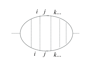
Figure 1: ladder diagrams in particle-hole channel, $i,j,k$ are band indices. We include only processes where particle and hole are coming from the same band.

Evaluating the diagrams, we obtain

$$\chi_{ii}(\vec{q},\omega)={(-i\omega+D_{\bar{i}}q^{2}+\tau_{\bar{i}i}^{-1})\rho_{ii}D_{i}q^{2}+\tau_{\bar{i}i}^{-1}\rho_{\bar{i}i}D_{\bar{i}}q^{2}\over(-i\omega+D_{2}q^{2}+\tau_{21}^{-1})(-i\omega+D_{1}q^{2}+\tau_{12}^{-1})-(\tau_{12}\tau_{21})^{-1}}$$ (8a)

and

$$\chi_{i\bar{i}}(\vec{q},\omega)={\tau_{\bar{i}i}^{-1}\left(\rho_{ii}D_{i}q^{2}+\rho_{\bar{i}i}D_{\bar{i}}q^{2}\right)\over(-i\omega+D_{2}q^{2}+\tau_{21}^{-1})(-i\omega+D_{1}q^{2}+\tau_{12}^{-1})-(\tau_{12}\tau_{21})^{-1}}$$ (8b)

where $D_{i}=v_{F}^{2}\tau_{i}/d$ is the diffusion constant for band $i$ electrons and

$$\rho_{ij}=P_{i}(0)P_{j}(0)N_{t}(0),\quad\leavevmode\nobreak\ P_{1(2)}(0)={N_{1(2)}(0)\over N_{t}(0)}.$$ (9)

where $N_{t}(0)=N_{1}(0)+N_{2}(0)$ is the total density of states on the Fermi surface. The result is valid in the small $q,\omega$ limit $\omega<<\tau_{i}^{-1}$ and $D_{i}q^{2}<<\tau_{i}^{-1}$ for both $i=1,2$.

$F_{ij}(q,\omega)$ can be evaluated using Eq. (8) and has very different behaviors at energy scales higher and lower than the inter-band scattering life-time $\tau_{i\bar{i}}^{-1}$. To simplify calculation we shall assume $\tau_{12}\sim\tau_{21}\sim\tau_{t}$ are of the same order of magnitude. In this case we obtain in the limit $\omega<<\tau_{t}^{-1}$ and $D_{i}q^{2}<<\tau_{t}^{-1}$,

$$F_{ij}(\vec{q},\omega)={\rho_{ij}D_{eff}q^{2}\over\omega^{2}+(D_{eff}q^{2})^{2}},$$ (10a)

where $$D_{eff}=P_{1}(0)D_{1}+P_{2}(0)D_{2}$$ and

$$F_{ij}(\vec{q},\omega)=\delta_{ij}N_{i}(0){D_{i}q^{2}\over\omega^{2}+(D_{i}q^{2})^{2}},$$ (10b)

in the opposite limit $\omega>>\tau_{t}^{-1}$ and $D_{i}q^{2}>>\tau_{t}^{-1}$. Physically, electrons have scattered many times between the two band already in the limit $\omega,D_{i}q^{2}<<\tau_{t}^{-1}$ and the identity of bands is lost as far as electron dynamics is concerned. The only remaining information of “bands” is that electrons have probability $P_{i}(0)$ of residing in band $i$. The identity of the two bands remain in the opposite limit $\omega,D_{i}q^{2}>>\tau_{t}^{-1}$ where electrons stay mainly in one-band. The two different limits expressed themselves in the GL equation where we find that in the limit $T_{c}<<\tau_{t}^{-1}$, electrons have to scatter between the two bands many times before forming a Cooper pair and the identity of intra-band Cooper pairs is lost, whereas intra-band Cooper pairs survived in the opposite limit $\tau_{t}^{-1}<<T_{c}$. We shall first consider the limit $T_{c}<<\tau_{t}^{-1}$ in the following.

Putting together Eqs. (4), (7) and (10) , we obtain

$$\bar{K}^{(0)}_{ij} \sim \sum_{k}V_{ik}\rho_{kj}\ln{\omega_{d}\over T},$$ (11)

$$\bar{K}^{(1)}_{ij} \sim -\sum_{k}V_{ik}\times\rho_{kj}{D_{eff}\over T_{c}}$$

where $\omega_{d}$ is the high energy cutoff for the attractive interaction in BCS theory. We have assumed $\tau_{t}^{-1}>>T_{c}$ in deriving $\bar{K}^{(1)}_{ij}$.

$\bar{L}^{(0)}_{ijkl}$ can be computed similarly in perturbation theory. We obtain after some lengthy algebra

$$\bar{L}^{(0)}_{ijkl}\sim-{1\over T_{c}^{2}}\sum_{m}V_{im}P_{m}(0)P_{j}(0)P_{k}(0)P_{l}(0)N_{t}(0).$$ (12)

The result can be understood most easily by noting that in the limit $T_{c}<<\tau_{t}^{-1}$ the dynamics of electron is described in an effective single-band picture with probability $P_{i}(0)$ of finding electrons in band $i$.

Putting Eqs. (4),  (11) and (12) in Eq. (Ginzburg-Landau theory of dirty two band $s_{\pm}$ superconductors), multiple the resulting equation by $P_{i}(0)$ and sum over $i$, we obtain an effective single band GL equation

$$\Delta_{eff}(\vec{r})=a(T)\Delta_{eff}(\vec{r})-{b\over 2}\nabla^{2}\Delta_{eff}(\vec{r})-c|\Delta_{eff}(\vec{r})|^{2}\Delta_{eff}(\vec{r})$$ (13)

where $\Delta_{eff}(\vec{r})=\sum_{i}P_{i}(0)\Delta_{i}(\vec{r})$ and $a(T)=V_{av}N_{t}(0)\ln(\omega_{d}/T)$, $b\sim V_{av}N_{t}(0)D_{eff}/T_{c}$, $c\sim V_{av}N_{t}(0)/T_{c}^{2}$ where $V_{av}=\sum_{ij}P_{i}(0)V_{ij}P_{j}(0)$ is the average interaction electrons see in forming the Cooper pairs.

The individual band order parameters $\Delta_{i}(\vec{r})$ are related to $\Delta_{eff}(\vec{r})$ by

$$\Delta_{i}(\vec{r})={1\over V_{av}}(\sum_{k}V_{ik}P_{k}(0))\Delta_{eff}(\vec{r}).$$ (14)

and are ‘slaved’ to $\Delta_{eff}$ in the sense that they are not independent dynamical variables in the system. The dirty two-band superconductor behaves as an effective dirty one-band superconductor in the regime $T_{c}<<\tau^{-1}_{t}$ where measurement of superfluid properties cannot distinguish between whether the system is originally a single-band or a two-band superconductor.

The effective single-band description has a number of interesting predictions. The (average) superconducting transition temperature is given by

$$T_{c}=\omega_{d}\exp(-(V_{av}N_{t}(0))^{-1}).$$ (15)

which is very different from clean two-band superconductors where $T_{c}$ is determined by

$$T_{c}^{(0)}=\omega_{d}\exp(-\left({\bar{V}_{11}+\bar{V}_{22}\over 2}+\sqrt{({\bar{V}_{11}-\bar{V}_{22}\over 2})^{2}+|\bar{V}_{t}|^{2}}\right)^{-1}),$$ (16)

where $\bar{V}_{ii}=V_{ii}N_{i}(0)$ and $\bar{V}_{t}=V_{t}\sqrt{N_{1}(0)N_{2}(0)}$ where $V_{t}=V_{12}=V_{21}$. Notice that $T_{c}^{(0)}$ is independent of $sgn(V_{t})$.

It is straightforward to show that $T_{c}\leq T_{c}^{(0)}$, i.e. $T_{c}$ is always lowered by disorder. However Eq. (15) says that the precise value of $T_{c}$ is insensitive to the strength of disorder and depends only on the density of states of the two Fermi surfaces in the limit $\tau_{t}^{-1}<<T_{c}$! This surprising result is a direct consequence of “Anderson Theorem”and applied to the (effective) one-band superconductor.

Contrary to the case of clean superconductors we also observe that $T_{c}$ depends now on the sign of $V_{t}$. In particular $T_{c}$ is enhanced by $V_{t}$ only if $V_{t}>0$, suggesting that disorder disfavor $s_{\pm}$ state. The relative sign between $\Delta_{1}$ and $\Delta_{2}$ depends on all the interactions now (Eq. (14)) and is not solely determined by $sgn(V_{t})$!

Next we consider the regime $\tau_{t}^{-1}\leq T_{c}$. This region is non-trivial as can be seen from the change in $T_{c}$ as a function of $\tau_{t}^{-1}$ determined by the GL theory. At $\tau_{t}^{-1}\rightarrow 0$ $T_{c}$ is determined by Eq. (16) for clean superconductors whereas $T_{c}$ is determined by Eq. (15) at $\tau_{t}^{-1}>>T_{c}$. $T_{c}$ is different but insensitive to disorder at both regimes (Anderson Theorem)! Therefore Anderson Theorem must breaks down and $T_{c}$ becomes sensitive to disorder at the intermediate regime $0\leq\tau_{t}^{-1}\leq T_{c}$. The non-trivial effect of impurity scattering in this regime is shown in single-impurity calculations where it is found that in-gap bound states are induced easily by inter-band impurity scattering and the Josephson coupling between the bands is suppressed correspondingly in the $s_{\pm}$ stateim1 ; im2 ; ng . We note that the in-gap states are absent in the $\tau_{t}^{-1}>>T_{c}$ limit where an effective single-band description becomes valid, consistent with findings on superconductors with sign-changing order-parameterspreosti .

The rare (but strong) effects of inter-band impurity scattering suggests that the self-averaging approximation $\langle K\Delta\rangle_{av}\sim\langle K\rangle_{av}\Delta$ breaks down in the regime $\tau_{t}^{-1}\leq T_{c}$ and $\Delta_{i}(\vec{r})$ becomes sensitive to the precise configuration of inter-band scattering potentials. The sensitivity of $\Delta_{i}(\vec{r})$ to the impurity potential can also be seen directly from the (averaged) GL equation. It is easy to show that

$$\bar{K}^{(1)}_{ij}\rightarrow-V_{ij}N_{j}(0)D_{i}/T_{c}.$$

and the GL equation does not take the form of an effective single-band GL equation in this regime. As a result its solutions are very sensitive to local variations in $K_{ij}^{(0)}(\vec{r})$.

Therefore to describe the effects of order at this regime we should start with the un-averaged equation (Ginzburg-Landau theory of dirty two band $s_{\pm}$ superconductors). It is more convenient is to replace the continuum GL equation by a random Josephson coupling lattice model with free energy

$$F = \sum_{i}\left(\sum_{ml}a_{ml}(T;i)(\Delta^{+}_{m}(i)\Delta_{l}(i)+c.c.)+\sum_{m}b_{m}|\Delta_{m}(i)|^{4}\right)$$

$$-\sum_{<ij>,l}t_{l}\left(\Delta^{+}_{l}(i)\Delta_{l}(j)+h.c.\right)$$

where $(i,j)$ and $(l,m)$ are lattice site and band indices, respectively. $<i,j>$ denotes nearest neighbor pair sites. The first term in (Ginzburg-Landau theory of dirty two band $s_{\pm}$ superconductors) represents grains of two-band superconductors where the two bands are coupled only through Josephson coupling $a_{12(21)}$. The second term represents Josephson coupling between nearest neighbor grains. $a_{lm}(T;i)\rightarrow a_{lm}(T)$ with $a_{12(21)}>0$ for clean $s_{\pm}$ superconductors and $a_{lm}$ becomes randomized in the presence of disorder. It is easy to see from a three-site calculation that the phase of the order parameters are frustrated if $sgn(a_{12(21)}(T;i))$ becomes randomizednn , indicating that a uniform superconducting state becomes unstable when inter-band impurity scattering is strong enough.

Experimentally, we note that different superconducting gaps were observed at energy bands located at the $\Gamma-$ and $M-$ points of the pnictide superconductors in ARPES experimentsARPES2 , indicating that the materials are located in the weak inter-band scattering regime $\tau_{t}^{-1}\leq T_{c}$ where impurity-induced in-gap bound states are present, consistent with the existence of large density of in-gap states found in NMRNMR1 and lower critical fieldfield experiments. We propose here that a uniform superconducting state may become unstable at this regime. A detailed analysis of the superconducting behavior at this regime will be the subject of a separate paper.

References

• (1) K. Seo, B.A. Bernevig and J. Hu, Phys.Β Rev.Β Lett.Β 101, 206404 (2008).
• (2) I.I. Mazin et.al., Phys.Β Rev.Β Lett.Β 101. 057003 (2008).
• (3) F. Wang et al., Phys.Β Rev.Β Lett.Β 102, 047005 (2009).
• (4) K.Matano ea al, Europhys. Lett. 83, 57001 (2008).
• (5) Cong Ren, et al, arXiv:0804.1726 (2008).
• (6) Lin Zhao et al, Chin. phys. Lett. 25 4402 (2008).
• (7) H. Ding et al, Europhys. Lett. 83, 47001 (2008).
• (8) Y. Bang, H.-Y. Choi and H. Won, Phys.Β Rev.Β B79, 054529 (2009).
• (9) D. Parker, O.V. Dolgov, M.M. Korshunov, A.A. Golubov and I.I. Mazin, Phys.Β Rev.Β B 78, 134524 (2008).
• (10) see for example P. G. de Gennes, Superconductivity of metals and Alloys, Benjamin, New York, 1966).
• (11) see for example P. A. Lee and T.V. Ramakrishnan, Rev. Mod. Phys. 57, 287 (1985).
• (12) N.R. Werhamer, E. Helfand, and P.D. Hohenberg, Phys. Rev. 147, 295 (1966).
• (13) G. Kotliar and A. Kapitulnik, Phys.Β Rev.Β B33, 3146 (1986).
• (14) P.W. Anderson, J. Phys. Chem. Solids 11, 26(1959).
• (15) T.K. Ng and Y. Avishai, arXiv:0906:2442.
• (16) G. Preosti and P. Muzikar, Phys.Β Rev.Β B54, 3489 (1995).
• (17) T.K. Ng and N. Nagaosa, arXiv:0809.3343.