Modulation and correlation lengths in systems with competing interactions

Abstract

We examine correlation functions in the presence of competing long and short ranged interactions to find multiple correlation and modulation lengths. We calculate the ground state stripe width of an Ising ferromagnet, frustrated by an arbitrary long range interaction. In large $n$ systems, we demonstrate that for a short range system frustrated by a general competing long range interaction, the crossover temperature $T^{*}$ veers towards the critical temperature of the unfrustrated short range system (i.e., that in which the frustrating long range interaction is removed) . We also show that apart from certain special crossover points, the total number of correlation and modulation lengths remains conserved. We derive an expression for the change in modulation length with temperature for a general system near the ground state with a ferromagnetic interaction and an opposing long range interaction. We illustrate that the correlation functions associated with the exact dipolar interactions differ substantially from those in which a scalar product form between the dipoles is assumed.

I Introduction

Short range interactions have been at the focus of much study for many decades. Perhaps one of the best known examples are the Ising ferromagnet and the anti-ferromagnet isi . Long range interactions are equally abundant lon . Systems in which both long and short range interactions co-exist comprise very interesting systems. Such competing forces can lead to a wealth of interesting patterns – stripes, bubbles, etc. lie , vin , ort , gul , bar (a). Realizations are found in numerous fields – quantum Hall systems Fog , adatoms on metallic surfaces, amphiphilic systems amp , interacting elastic defects (dislocations and disclinations) in solids vor (a), interactions amongst vortices in fluid mechanics vor (b) and superconductors vor (c), crumpled membrane systems Seu , wave-particle interactions wav , interactions amongst holes in cuprate superconductors ste , us , zoh (a), Löw et al. (1994), car , arsenide superconductors nas , manganates and nickelates che , gol , some theories of structural glasses Kivelson et al. (1995), pet , Gil , new , rev , colloidal systems der , rei and many many more. Much of the work to date focused on the character of the transitions in these systems and the subtle thermodynamics that is often observed (e.g., the equivalence between different ensembles in many such systems is no longer as obvious, nor always correct, as it is in the canonical short range case bar (b)). Other very interesting aspects of different systems have been addressed in azb .

Here we investigate the general temperature dependence of the structural features that appear in such systems when competing interactions of short and long range are present. Our focus here is on large $n$ spin systems. In many such systems, there are emergent modulation lengths governing the size of various domains. We find that these modulation lengths often adhere to various scaling laws, sharp crossovers and divergences at various temperatures (with no associated thermodynamic transition). We also find that in such systems, correlation lengths generically evolve into modulation lengths (and vice versa) at various temperatures. The behavior of correlation and modulation lengths as a function of temperature will afford us with certain selection rules on the possible underlying microscopic interactions. In their simplest incarnation, our central results are as follows:

1. In canonical systems harboring competing short (finite) and long range interactions modulated patterns appear. Depending on the type of the long range interaction, the modulation length either increases or decreases from its ground state value as the temperature is raised. We will relate this change, in lattice systems, to derivatives of the Fourier transforms of the interactions that are present.

2. There exist special crossover temperatures at which new correlation/modulation lengths come up or some cease to exist. The total number of characteristic length-scales (correlation + modulation) remains conserved, except at the crossover points.

3. The presence of the angular dependent dipolar interaction term that frustrates an otherwise unfrustrated ferromagnet vis a vis a simple scalar product between the dipoles adds new (dominant) length-scales. The angular dependence significantly changes the system.

We will further investigate the ground state modulation lengths in general frustrated Ising systems and also point to discontinuous jumps in the modulation lengths that may appear in the large $n$ rendition of some systems.

Armed with these general results, we may discern the viable microscopic interactions (exact or effective) which underlie temperature dependent patterns that are triggered by two competing interactions. Our analysis suggests the effective microscopic interactions that may drive non-uniform patterns such as those underlying lattice analogs of the systems of Fig. 1.

The treatment that we present in this work applies to lattice systems and does not account for the curvature of bubbles and other continuum objects. These may be augmented by inspecting energy functionals (and their associated free energy extrema) of various continuum field morphologies under the addition of detailed domain wall tension forms – e.g., explicit line integrals along the perimeter where surface tension exists – and the imposition of additional constraints via Lagrange multipliers. We leave their analysis for future work. One of the central results of our work is the derivation of conditions relating to the increase/decrease of modulation lengths in lattice systems with changes in temperature. These conditions relate the change in the modulation length at low temperatures to the derivatives of the Fourier transforms of the interactions present.

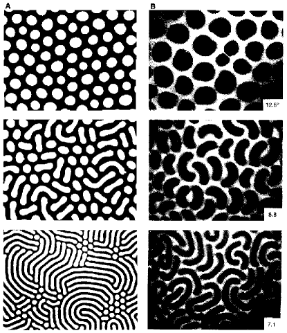
Figure 1: Reproduced with permission from Science, Ref.Seu . Reversible “strip-out” instability in magnetic and organic thin films. Period ($L_{D}$) reduction under the constraint of fixed overall composition and fixed number of domains leads to elongation of bubbles. Left panel (A) in magnetic garnet films, this is achieved by raising the temperature [labeled in (B) in degrees Celsius] along the symmetry axis, $H=0$ (period in bottom panel, $\sim 10\mu m$) (see Fig. 5). Right panel (B) In Langmuir films composed of phospholipid dimyristolphosphatidic acid (DMPA) and cholesterol (98:2 molar ratio, pH 11), this is achieved by lowering the temperature at constant average molecular density [period in bottom panel, $\sim 20\mu m$]

.

In Section(II), we outline the general systems that we study. In particular, we introduce the frustrated ferromagnet.

In Section(III), we derive the scaling form for the Ising ground states for general frustrating long range interactions. Henceforth, we provide explicit expressions for the crossover temperatures and the correlations lengths in the large $n$ limit.

In Section(IV), we introduce the two spin correlation function for a general system in this limit.

Based on the correlation function, we then present some general results for systems with competing nearest neighbor ferromagnetic interaction and an arbitrary long range interaction in Section(V). We start by deriving the equilibrium stripe width for a two dimensional Ising system with nearest neighbor ferromagnetic interactions and competing long range interactions. We derive an expression for the change in modulation length with temperature for low temperatures for large $n$ systems. We illustrate how the crossover temperature, $T^{*}$ arises in the large $n$ limit and show some general properties of the system associated with it.

We present some example systems in Section(VI). We numerically calculate the correlation function for the screened Coulomb frustrated ferromagnet and the dipolar frustrated ferromagnet. We then study the screened Coulomb frustrated ferromagnet in more details. Next, we show some results for systems with higher dimensional spins. We study a system with the dipole-dipole interaction for three dimensional spins, without ignoring the angular dependent term and show that this term changes the ground state length-scales of the system considerably. We also present a system with the Dzyaloshinsky - Moriya interaction in addition to the ferromagnetic term and a general frustrating long range term.

We give our concluding remarks in Section(VII).

II The systems of study

Consider a translationally invariant system whose Hamiltonian is given by

$$H=\frac{1}{2}\sum_{\vec{x}\neq\vec{y}}V(|\vec{x}-\vec{y}|)S(\vec{x})S(\vec{y}).$$ (1)

The quantities $\{S(\vec{x})\}$ portray classical scalar spins or fields. The sites $\vec{x}$ and $\vec{y}$ lie on a hypercubic lattice with $N$ sites having unit lattice constant. In what follows, $v(k)$ and $s(\vec{k})$ will denote the Fourier transforms of $V(|\vec{x}-\vec{y}|)$ and $S(\vec{x})$. Thus, we have,

$$H=\frac{1}{2N}\sum_{\vec{k}}v(k)|s(\vec{k})|^{2}$$ (2)

For analytic interactions, $v(k)$ is a function of $k^{2}$ (to avoid branch cuts).

The two point correlator function for the system in Eq. (1) is,

$$G(\vec{x})=\langle S(0)S(\vec{x})\rangle$$ (3)

Thus, in the Fourier space, we have,

$$G(\vec{k})=\langle|s(\vec{k})|^{2}\rangle$$ (4)

Throughout most of this work we will focus on systems with competing interactions having Hamiltonians of the following form.

$$H=-J\sum_{\langle\vec{x},\vec{y}\rangle}S(\vec{x})S(\vec{y})+Q\sum_{\vec{x}\neq\vec{y}}V_{L}(|\vec{x}-\vec{y}|)S(\vec{x})S(\vec{y}),$$ (5)

where the first term represents nearest neighbor ferromagnetic interaction for positive $J$ and the second term represents some long range interaction which opposes the ferromagnetic interaction for positive $Q$. We will study properties of general systems of the form of Eq.(5). In order to flesh out the physical meaning of our results and illustrate their implications and meaning, we will further provide explicit expressions and numerical results for two particular examples. The Hamiltonian of Eq.(5) represents a system that we christen to be the screened Coulomb Frustrated Ferromagnet when

$$V_{L}(r)=\frac{e^{-\lambda r}}{4\pi r}\mbox{ in three dimensions, and}$$

$$V_{L}(r)=K_{0}(\lambda r)\mbox{ in two dimensions,}$$ (6)

where $\lambda^{-1}$ represents the screening length and $K_{0}$ is a modified Bessel function,

$$K_{0}(x)=\int_{0}^{\infty}dt\frac{\cos xt}{\sqrt{1+t^{2}}}.$$ (7)

Throughout our work, we will discuss both the screened and unscreened renditions of the Coulomb frustrated ferromagnet. Eq.(5) corresponds to a Dipolar Frustrated Ferromagnet when

$$V_{L}(r) = \frac{1}{r^{3}}$$ (8)

$$= \frac{1}{(r^{2}+\delta^{2})^{3/2}}\mbox{ in the limit }\delta\to 0,$$

on the lattices that we will consider. Later, we also consider the general direction dependent (relative to the location vectors) of the dipolar interaction for three dimensional spins; we will replace the scalar product form of the dipolar interactions in Eqs.(5, 8) by the precise dipolar interactions between magnetic moments.

On a hypercubic lattice, the nearest neighbor interactions in real space of Eq.(5) have the lattice Laplacian

$$\Delta(\vec{k})=2\sum_{l=1}^{d}(1-\cos k_{l}),$$ (9)

as their Fourier transform. In the continuum (small $k$) limit, $\Delta\to z=k^{2}$. The real lattice Laplacian

$$\langle\vec{x}|\Delta|\vec{y}\rangle=\left\{\begin{array}[]{ll}2d&\mbox{ for $\vec{x}=\vec{y}$}\\ -1&\mbox{ for $|\vec{x}-\vec{y}|=1$.}\end{array}\right.$$ (10)

Notice that $\langle\vec{x}|\Delta^{R}|\vec{y}\rangle=0\mbox{ for $|\vec{x}-\vec{y}|>R$}$, where $R$ is the spatial range over which the interaction kernel is non-vanishing. The following corresponds to interactions of Range=2 lattice constants,

$$\langle\vec{x}|\Delta^{2}|\vec{y}\rangle\mbox{ }=\mbox{ } 2d(2d+2)\mbox{ for }\vec{x}=\vec{y}$$

$$-4d\mbox{ for }|\vec{x}-\vec{y}|=1$$

$$2\mbox{ for }(\vec{x}-\vec{y})=(\pm\hat{e}_{\ell}\pm\hat{e}_{\ell^{\prime}})\mbox{ where }\ell\neq\ell^{\prime}$$

$$1\mbox{ for a $\pm 2\hat{e}_{\ell}$ separation}.$$ (11)

Correspondingly, in the continuum, the Lattice Laplacian and its powers attain simple forms and capture tendencies in numerous systems. Surface tension in many systems is captured by a $g(\nabla\phi)^{2}$ term where $\phi$ is a constant in a uniform domain. Upon Fourier transforming, such squared gradient terms lead to a $k^{2}$ dependence. The effects of curvature which are notable in many mixtures and membrane systems can often be emulated by terms involving $(\nabla^{2}h)$ with $h$ a variable parameterizing the profile; at times the interplay of such curvature terms with others leads, in the aftermath, to a simple short range $k^{4}$ term in the interaction kernel (the continuum version of the squared lattice Laplacian of Eq.(11)). An excellent review of these issues is addressed in Seu .

III Ground state stripe width for Ising systems

We next briefly discuss the ground state stripe width for systems with general long range interactions in Eq.(5). Below, we discuss the Ising ground states. We will later on consider the spherical model that will enable us to compute the correlation functions at arbitrary temperatures. We consider a system with Ising spins in $d$ dimension and assume that the system forms a “striped” pattern (periodic pattern along one of the dimensions – stripes in two dimensions, parallel slices in three dimensions and so on) of spin-up and spin-down states of period $l$. We then calculate the free energy as a function of $l$ and then minimize it with respect to $l$ to get the equilibrium stripe width. For the frustrated ferromagnet, if $v_{L}(k)=1/k^{p}$,

$$l=\left[\frac{(2\pi)^{p+2}J}{4Qp\left(1-\frac{1}{2^{p+2}}\right)\zeta(p+2)}\right]^{\frac{1}{p+1}},$$ (12)

where $\zeta(s)$ is the Riemann zeta function,

$$\zeta(s)=\sum_{n=1}^{\infty}n^{-s}.$$ (13)

For the particular case of Coulomb frustration, $p=2$,

$$l=\sqrt[3]{\frac{64\pi^{2}}{5}\frac{J}{Q}},$$ (14)

in accord with the results of Refs. Gil ; zoh (b). For long range dipolar interactions ($p=3$), we find that

$$l=\delta\sqrt{\frac{3J}{Q}}.$$ (15)

In the notation to be employed later on in this work, $l$ plays the role of the modulation length of the system at zero temperature, $L_{D}(T=0)$.

IV Correlation Functions in the large $n$ limit - general considerations

The results reported henceforth were computed within the spherical or large $n$ limit kac . It was found by Stanley long ago Stanley (1968) that the large $n$ limit of the $n$ component normalized spin systems (so called $O(n)$ spins) is identical to the spherical model first introduced by Berlin and Kac kac .

The designation of “$O(n)$ spins” simply denotes real fields (spins) of unit length that have some arbitrary number $(n)$ of components. For $n=1$, the system is an Ising model. A single component real field having unit norm allows for only two scalars at any given site $\vec{x}$: $S(\vec{x})=\pm 1$. The $n=2$ system corresponds to a two component spin system in which the spins are free to rotate in a two dimensional place – $S_{1}^{2}(\vec{x})+S_{2}^{2}(\vec{x})=1$ (the so-called XY spin system). The case of $n=3$ corresponds to a system of three component Heisenberg type spins, and so on. In general,

$$\sum_{a=1}^{n}S_{a}(\vec{x})S_{a}(\vec{x})=1.$$ (16)

We now introduce the spherical model in its generality. The spins in Eq.(1) satisfy a single global (“spherical”) constraint,

$$\sum_{\vec{x}}\langle S^{2}(\vec{x})\rangle=N,$$ (17)

enforced by a Lagrange multiplier $\mu$. This leads to the functional $H^{\prime}=H+\mu N$ which renders the model quadratic (as both Eqs.(1, 17) are quadratic) and thus exactly solvable, see, e.g., us . The continuum analogs of Eqs.(1, 17) read

$$H=\frac{1}{2}\int d^{d}x~{}d^{d}y~{}V(|\vec{x}-\vec{y}|)S(\vec{x})S(\vec{y}),$$

$$\int d^{d}x~{}\langle S^{2}(\vec{x})\rangle=const.$$ (18)

The quadratic theory may be solved exactly. From the equipartition theorem, for $T\geq T_{c}$, the Fourier space correlator

$$G(k)=\langle|S^{2}(k)|\rangle=\frac{k_{B}T}{v(k)+\mu}.$$ (19)

The real space two point correlator is given by

$$G(\vec{x})\equiv\langle S(0)S(\vec{x})\rangle=k_{B}T\int_{BZ}\frac{d^{d}k}{(2\pi)^{d}}\frac{e^{i\vec{k}\cdot\vec{x}}}{v(k)+\mu},$$ (20)

with $d$ the spatial dimension and $BZ$ denoting the integration over the first Brillouin zone. For a hypercubic lattice in $d$ dimensions with a lattice constant that is set to one, $-\pi<k_{i}\leq\pi$ for $i=1,2,...,d$. Henceforth, to avoid cumbersome notation, we will generally drop the designation of $BZ$; this is to be understood on all momentum space integrals pertaining to the lattice systems that we examine. To complete the characterization of the correlation functions at different temperatures, we note that the Lagrange multiplier $\mu(T)$ is given by the implicit equation $1=G(\vec{x}=0)$. Thus,

$$1=k_{B}T\int\frac{d^{d}k}{(2\pi)^{d}}\frac{1}{v(k)+\mu}.$$ (21)

This implies that the temperature $T$ is a monotonic increasing function of $\mu$. If $\mu$ changes by a small amount $\Delta\mu$, then $T$ will change by an amount $\Delta T$, such that

$$\Delta T\propto\Delta\mu.$$ (22)

Eq.(21) also implies that in the high temperature limit,

$$\frac{\mu}{k_{B}T} = \frac{\pi^{d/2}\Lambda^{d}}{(2\pi)^{d}\Gamma(\frac{d}{2}+1)}$$ (23)

$$\implies T \propto \mu,$$ (24)

where $\Lambda$ is the upper limit of the $k$ integration, representing the ultra-violet cut-off in continuum renditions of the large $n$ system. Similarly, if we perform, for a lattice system, the momentum integration in a hypercube of side $2\pi$, we have in the high temperature limit,

$$\mu=k_{B}T.$$ (25)

Furthermore, as the integration range in Eq. (21) is finite, we can prove that $\mu(T)$ is an analytic function of $T$ [See Appendix D]. This supports the assumption that $G^{-1}(T,k)$ is analytic in $T$ and $k$ at all points except $k=0$ where $v(k)$ is usually singular.

We investigate the general character of the correlation functions given by Eq.(20) for rotationally invariant systems. If the minimum (minima) of $v(k)$ occur(s) at momenta $q$ far from the Brillouin zone boundaries of the cubic lattice then we may set the range of integration in Eq.(20) to be unrestricted. The correlation function is then dominated by the location of the poles (and/or branch cuts) of $1/[v(k)+\mu]$. Thus, we look for solutions to the following equation.

$$v(k)+\mu=0.$$ (26)

The system is perfectly ordered in its ground state. From a temperature at which the system is not perfectly ordered, as we lower the temperature, the correlation length diverges at $T=T_{c}$. At $T=T_{c}$, $\mu$ takes the value,

$$\mu_{min}=-\min_{k\in BZ}[v(k)].$$ (27)

As the temperature is increased, the disorder creeps in and in many systems, at a temperature $T^{*}$, the modulation length diverges.

The characteristic length-scales of the system are governed by the poles of $[v(k)+\mu]^{-1}$.

$$J\Delta(\vec{k})+Qv_{L}(k)+\mu=0,$$ (28)

which in the continuum limit takes the form

$$Jk^{2}+Qv_{L}(k)+\mu=0.$$ (29)

Employing the above considerations, we will derive, in the next section, some general results for systems of the form Eq.(5).

Our work will focus on classical systems. The extension to the quantum arena us is straightforward. In, e.g., large $n$ bosonic renditions of our system, replicating the usual large $n$ analysis, we find new that the pair correlator

$$G_{B}(\vec{k})=\frac{n_{B}\left(\sqrt{\frac{v(\vec{k})+\mu}{k_{B}T}}\right)+\frac{1}{2}}{\sqrt{\frac{v(\vec{k})+\mu}{k_{B}T}}},$$ (30)

with the bosonic distribution function

$$n_{B}(x)=\frac{1}{e^{x}-1}.$$ (31)

The correlator of Eq.(30) is of a similar nature as that of the classical correlator of Eq.(19) with branch cuts generally appearing in the quantum case. Our analysis below relies on the evolution of the poles of $v(k)+\mu$ as a function of temperature in classical systems.

In the quantum arena, we first choose the proper contour in the complex $k$-space (going around the branch cuts). Then, we argue that the only points that contribute to the integral are the points where the integrand is singular. This corresponds to $v(k)+\mu=0$. Thus, the integral remains unchanged if we expand the integrand to lowest order in $v(k)+\mu$. Doing this, we get, to leading order,

$$G_{B}(k)=\frac{k_{B}T}{v(k)+\mu}$$ (32)

which is same as the classical expression. The characteristic length-scales of the system are therefore still determined by the zeros of $v(k)+\mu$ in the complex $k$ plane in the exact same way.

For interactions that are not isotropic, for both classical and quantum cases, we need to consider the full six dimensional space of the complex components of $\vec{k}$ along each of the three coordinate axes.

V Large $n$ Results

In this section, we present some general results for systems of the form Eq.(5) in their large $n$ limit. First, we find the dependence of the modulation length on temperature, near $T_{c}$. Next, we will illustrate an analogy between the behavior of the correlation length near the critical temperature $T_{c}$ and that of the modulation length near $T^{*}$. We will then discuss some aspects of the crossover points. We end this section with some results in the high temperature limit.

V.1 The low temperature limit: a criterion for determining an increase or decrease of the modulation length at low temperatures

In this section, we derive universal conditions for increasing or decreasing modulation lengths in general systems pairwise interactions. Eqs.(43, 45) show general conditions for the change in modulation length, $L_{D}$ with temperature for a general system of the form Eq.(5). The value, $k_{0}$ of $k$ which satisfies Eq.(27),

$$v(k_{0})=\min_{k\in BZ}v(\vec{k})$$ (33)

determines the modulation length at $T=T_{c}$.

$$v(k_{0})+\mu_{min}=0,$$ (34)

$$v^{\prime}(k_{0})=0.$$ (35)

As the temperature is raised, the new pole near $k_{0}$ will have an imaginary part corresponding to the finite correlation length. The real part will also change in general and this would induce a change in the modulation length. Let $\mu(T)=\mu_{min}+\delta\mu$ with $\delta\mu>0$. Then we have,

$$k=k_{0}+\delta k,$$

$$\delta k=\sum_{j=1}^{\infty}\delta k_{j},$$ (36)

where $\delta k_{j}\propto\delta\mu^{x_{j}}$, $x_{j+1}>x_{j}$. Our goal is to find the leading order real contribution to $\delta k$ which would give us the change in modulation length with increasing $\mu$ and hence with increasing temperature.

$$\sum_{j=2}^{\infty}v^{(j)}(k_{0})\frac{\delta k^{j}}{j!}+\delta\mu=0.$$ (37)

Suppose $v^{(n)}(k_{0})=0$ for $2<n<p$ and $v^{(p)}(k_{0})\neq 0$. [Clearly, in most cases, the third derivative is not zero and $p=3$.] We have,

$$\frac{v^{(2)}(k_{0})}{2!})(\delta k_{1}^{2}+2\delta k_{1}\delta k_{2}+...)$$

$$+[\frac{v^{(p)}(k_{0})}{p!}(\delta k_{1}^{p}+p\delta k_{1}^{p-1}\delta k_{2}+...)+\frac{v^{(p+1)}(k_{0})}{(p+1)!}\times$$

$$(\delta k_{1}^{p+1}+(p+1)\delta k_{1}^{p}\delta k_{2}+...)+...]+\delta\mu=0.\ \$$ (38)

To leading order,

$$\frac{v^{(2)}(k_{0})}{2!}\delta k_{1}^{2}+\delta\mu=0,$$

$$\delta k_{1}^{2}=-\frac{2\delta\mu}{v^{(2)}(k_{0})}.$$ (39)

From this, we see that $\delta k_{1}$ is imaginary. This constitutes another verification of the well established result about the universality of the divergence of the correlation length, $\xi$ at $T_{c}$ with the mean-field type critical exponent $\nu=1/2$ in the large $n$ limit.

$$\xi\propto(T-T_{c})^{-\nu},$$

$$\nu=\frac{1}{2}.$$ (40)

The next, higher order, relations are obtained using the method of dominant balance.

$$v^{(2)}(k_{0})(\delta k_{1})(\delta k_{2})+\frac{v^{(p)}(k_{0})}{p!}(\delta k_{1})^{p}=0$$

$$\delta k_{2}=\frac{(-1)^{\frac{p+1}{2}}v^{(p)}(k_{0})(\delta\mu)^{\frac{p-1}{2}}}{2p!(\frac{v^{(2)}(k_{0})}{2!})^{\frac{p+1}{2}}}.$$ (41)

Therefore, $\delta k_{2}$ is real if $p$ is odd and imaginary if $p$ is even. If,

$$L_{D}(T)=L_{D}(T_{c})+\delta L_{D},$$ (42)

then, for $p=2n+1$,

$$\delta L_{D}=\frac{2\pi}{k_{0}^{2}}\frac{(-1)^{n}v^{(2n+1)}(k_{0})\delta\mu^{n}}{2(2n+1)!(\frac{v^{(2)}(k_{0})}{2!})^{n+1}}.$$ (43)

Thus to get the leading order real contribution to $\delta k$ for even $p$$[>2]$, we have to go to higher order.

$$2(\frac{v^{(2)}(k_{0})}{2!})\delta k_{1}\delta k_{3}+\frac{v^{(p+1)}(k_{0})}{(p+1)!}\delta k_{1}^{p+1}=0$$

$$\delta k_{3}=\frac{(-1)^{1+p/2}v^{(p+1)}(k_{0})(\delta\mu)^{p/2}}{2(p+1)!(\frac{v^{(2)}(k_{0})}{2!})^{p/2+1}}.$$ (44)

For $p=2n$,

$$\delta L_{D}=\frac{2\pi}{k_{0}^{2}}\frac{(-1)^{n}v^{(2n+1)}(k_{0})(\delta\mu)^{n}}{2(2n+1)!(\frac{v^{(2)}(k_{0})}{2!})^{n+1}}.$$ (45)

If, for $p=2n$, $v^{(2n+1)}(k_{0})=0$, then we will need to continue this process until we get a real contribution to $\delta k$. In appendix B, we provide explicit forms for $\delta L_{D}$ for different values of $p$.

In the most common case, where $v^{(3)}(k_{0})\neq 0$, we have,

$$\delta L_{D}=-\frac{2\pi}{k_{0}^{2}}\frac{v^{(3)}(k_{0})}{3[v^{(2)}(k_{0})]^{2}}\delta\mu.$$ (46)

Also, applying this to a nearest neighbor system in the continuum frustrated by a general long range interaction given by $v_{L}(k)$ in Fourier space , we get,

$$\delta L_{D}=-\frac{2\pi}{k_{0}^{2}}\frac{Qv_{L}^{(3)}(k_{0})}{3[v_{L}^{(2)}(k_{0})]^{2}}\delta\mu.$$ (47)

This shows that it is the long range term that determines the sign of the change in modulation length with temperature as the system is heated from $T=T_{C}$. The results derived above allow us to relate an increase/decrease in the modulation length at low temperatures to the sign of the first non-vanishing odd derivative (of an order larger than two) of the Fourier transform of the interactions that are present. It is important to emphasize that our results apply to any interaction. These may include screened or unscreened Coulomb and other long range interactions but may also include interactions that are strictly of finite range [e.g., next-nearest neighbor interactions on the lattice for which we have $v_{L}=-t\Delta^{2}$ (with a constant $t>0$, see Eq.(11))].

The results from this section about modulation lengths just above $T_{C}$, can give us similar behavior of the correlation lengths at temperatures slightly below $T^{*}$.

V.2 A correspondence between the temperature $T^{*}$ at which the modulation length diverges and the critical temperature $T_{c}$

The critical temperature $T_{c}$ corresponds to the maximum value of $\mu$ for which Eq.(26) still attains a real solution. Thus,

$$v(k_{0})+\mu_{min}=0,$$

$$v^{\prime}(k_{0})=0,$$

$$v^{\prime\prime}(k_{0})>0.$$ (48)

For systems in which the modulation length diverges at $T^{*}$, $T^{*}$ corresponds to the minimum value of $\mu$ for which Eq.(26) has a purely imaginary solution. Thus, if $v(i\kappa)=\hat{v}(\kappa)$,

$$\hat{v}(\kappa_{0})+\mu^{*}=0$$

$$\hat{v}^{\prime}(\kappa_{0})=0$$

$$\hat{v}^{\prime\prime}(\kappa_{0})<0\implies v^{\prime\prime}(i\kappa_{0})>0$$ (49)

Thus, we expect similar qualitative results for the correlation lengths at temperatures slightly above $T_{c}$ as for modulation lengths slightly below $T^{*}$ and vice-versa. [The relations for the derivatives of $\hat{v}(\kappa_{0})$ in Eq.(49) are guaranteed to hold only if $T^{*}>T_{c}$.]

V.3 Crossover temperatures: Emergent modulations

For systems with competing multiple range interactions, there may exist special temperatures at which the poles of the correlation function change character, thus changing modulation lengths to correlation lengths and vice-versa. In particular, for most systems we have a crossover temperature $T^{*}$ above which the system does not have any modulation. Apart from this kind of phenomenon, there might also be finite discontinuous jumps in the modulation length. This is illustrated with an example in Section(V.4).

We start by defining the crossover temperature $T^{*}$ for a ferromagnetic system frustrated by a general long range interaction. Let $k=i\kappa$, $\kappa\in\mathbb{R}$ above $T^{*}$ and $\kappa=\kappa_{0}$ at $T^{*}$. Let $v(k)=f(z)$, $z=k^{2}$. Above $T^{*}$, $\mu=\mu_{min}+\Delta\mu$ [$\Delta\mu>0$]. Using Eq.(27),

$$\mu=-f(-\kappa^{2}) = -\min_{k\in\mathbb{R}}v(k)+\Delta\mu$$ (50)

$$= \max_{k\in\mathbb{R}}[-v(k)]+\Delta\mu.$$

$T^{*}$ corresponds to the minimum value of $\Delta\mu$ for which we have at least one such solution. See Fig. 2.

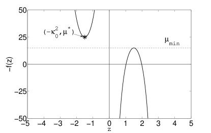
Figure 2: $-f(z)=-v(k)=\mu$ plotted against $z=k^{2}$ for purely real and purely imaginary $k$’s ($T\to 0$ and $T\to\infty$ respectively). The negative $z$ regime corresponds to temperatures (Lagrange multiplier, $\mu$’s) for which purely imaginary solutions exist. The maximum of the curve in the positive $z$ regime corresponds to the modulations at $T=T_{c}$ [$\mu=\mu_{min}$], which is the maximum temperature at which pure modulations exist.

Thus,

$$\mu^{*} = \min_{\begin{array}[]{c}\kappa\in\mathbb{R}\\ -v(i\kappa)\geq\mu_{min}\end{array}}[-v(i\kappa)]$$ (53)

$$= -\max_{\begin{array}[]{c}\kappa\in\mathbb{R}\\ -v(i\kappa)\geq\mu_{min}\end{array}}[v(i\kappa)].$$ (56)

Sometimes, the crossover point is slightly more difficult to visualize. See Fig. 3. In this case, the minimum upper branch of $-f(z)$ for $z<0$ [equivalently the upper branches of $-v(i\kappa)$] gives us the value of $\mu^{*}$. The branch chosen has to continue to $\mu=+\infty$ so that at least one term without modulation is always available as we increase the temperature, as required by the definition of $T^{*}$. The other branch provides such solutions only up to a certain temperature. Also, the part of it which is below $\mu_{min}$ is irrelevant.

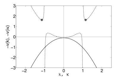
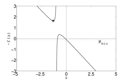
Figure 3: TOP: Solid line:$-v(k)$ plotted against $k$.
Dashed line:$-v(i\kappa)$ plotted against $\kappa$.
BOTTOM: $-f(z)$ plotted against $z$.

If $f(z)$ is an odd function of $z$ (e.g. the Coulomb frustrated ferromagnet), $\mu^{*}=-\mu_{min}$ and the correlation length at $T^{*}$ is the same as the modulation length at $T_{c}$.

Also, for the system in Eq.(5), if $\lim_{\kappa\to 0}v_{L}(i\kappa)=+\infty$, we have, $\mu^{*}=\mu_{min}$, and $T^{*}=T_{c}$.

V.3.1 $T^{*}=T_{c}$ if all the competing interactions are of finite range and crossover exists

For systems where all the competing interactions are of finite range, $T^{*}=T_{c}$. We prove this as follows. Since finite range interactions contribute to $v(k)$ as powers of $\Delta(k)\to k^{2}$, for a system with only finite range interactions, $f(z)$ is analytic for all $z$. For a minimum of $-f(z)$ to exist in the $z<0$ regime which is higher than the maximum in the $z>0$ regime, we need $f(z)$ to be discontinuous at some point. Putting all of the pieces together, we find that there are no possibilities: (i) no crossover, i.e., $T^{*}=\infty$ or (ii) $\kappa_{0}=0$ and $\mu^{*}=\mu_{min}$ with $T^{*}=T_{c}$.

V.3.2 $T^{*}\to T_{c}$ as the strength of the long range interaction is turned off

The results from this section and the next hold for a general system, not just the frustrated ferromagnet.

The crossover temperature $T^{*}$ tends to $T_{c}$ for $Q=0$ as $Q\to 0$. For a general system, let $G(T,k)$ denote the Fourier space correlation function at temperature $T$. By definition, at $T=T_{c}$ the correlation length is infinite. Thus, $T_{c}$ is the solution to

$$G^{-1}(T,k)=0,$$ (57)

such that $k\in BZ$ (or for continuum renditions, $k\in\mathbb{R}$).

$T^{*}$ is the temperature at which the modulation length diverges for the frustrated ferromagnet, or becomes the same as the modulation length of the unfrustrated system at $T_{c}$ for a general system. Thus, $T^{*}$ is the solution to

$$G^{-1}(T,q+i\kappa)=0,$$ (58)

with $\kappa\in\mathbb{R}$ [$q=0$ for the case of the frustrated ferromagnet, $q=\pi$ for the frustrated anti-ferromagnet]. At $T_{c}$, for $Q=0$, we have,

$$G^{-1}(T_{c},q)=0.$$ (59)

This however also satisfies Eq.(58), with $\kappa=0$. Therefore,

$$\lim_{Q\to 0}T^{*}=T_{c}.$$ (60)

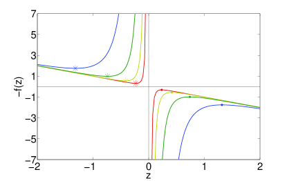
Figure 4: (Color online.) Illustration of the limit $T^{*}\to T_{c}$ as $Q\to 0$ with $v_{L}(k)=1/k^{3}$. The plot shows $-f(z)=-v(k)$ vs $z=k^{2}$, for $v(k)=Jk^{2}+Q/k^{3}$ with $J=1$ and $Q=\{1-$Blue, $0.1-$Green, $0.01-$Yellow, $0.001-$Red$\}$. ‘*’ represents the value of $\mu^{*}$ and dot represents $\mu_{min}$.

We demonstrate this in the large $n$ limit. See Fig. 4. For $Q=0$, we have $\mu_{min}=0$ and $k_{0}=0$. Let $v_{L}(k)$ diverge as $k^{-2p}$ near $k=0$. For small $Q$, from Eq.(27), we have,

$$k_{0}=(\frac{pQ}{J})^{\frac{1}{2p+2}},$$

$$\mu_{min}=-\frac{p+1}{p^{\frac{p}{p+1}}}J^{\frac{p}{p+1}}Q^{\frac{1}{p+1}}.$$ (61)

If $p$ is odd,

$$\mu^{*}=-\mu_{min},$$

$$\kappa_{0}=k_{0}.$$ (62)

As $Q\to 0$, $\kappa_{0}=k_{0}=0$ and $\mu^{*}=\mu_{min}=0$, that is,

$$\lim_{Q\to 0}T^{*}=T_{c}(Q=0).$$ (63)

V.3.3 Proof of the conservation of the total number of characteristic length-scales

In this section we consider the general situation in which the Fourier transform of the interaction kernel, $v(k)$, is a rational function of $z=\Delta(k)$, [$z\to k^{2}$ in the continuum limit]. That is, we consider situations for which

$$v(k)=f(z)=\frac{P(z)}{Q(z)},$$ (64)

with $P$ and $Q$ polynomials (of degrees $M_{1}$ and $M_{2}$ respectively). We will now demonstrate that the combined sum of the number of correlation and the number of modulation lengths remains unchanged as the temperature is varied.

Before providing the proof of our assertion, we first re-iterate that the form of Eq.(64) is rather general. For a system with finite range interactions ($V(|\vec{x}-\vec{y}|>R)=0$ with finite $R$) that is even under parity ($V(\vec{x}-\vec{y})=V(\vec{y}-\vec{x})$), the Fourier transform of $V(\vec{x}-\vec{y})$ can be written as a finite order polynomial in $(1-\cos k_{l})$ with the spatial direction index $1\leq l\leq d$ where $d$ is the dimensionality. In the small $|\vec{k}|$ (continuum limit), $[1-\cos k_{l}]\to k_{l}^{2}/2$. The particular case of a system with only finite range interactions that exist up to a specified range $R$ on the lattice (the range being equal to a graph distance measuring the number of lattice steps beyond which the interactions vanish) of the form of Eq.(64) corresponds to $v(k)=P(z)$ with the order of the polynomial $M_{1}$ being equal to the interaction range, $R=M_{1}$. Our result below includes such systems as well as general systems with long range interactions. For long range interactions such as, e.g., the screened Coulomb frustrated ferromagnet, $f(z)=1/(z+\lambda^{2})$. The considerations given below apply to the correlations along any of the spatial directions $l$ (and as a particular case, radially symmetric interactions for which the correlations along all directions attain the same form).

Returning to the form of Eq.(64), the Fourier space correlator of Eq.(19) is given by

$$G(\vec{k})=k_{B}T\frac{Q(z)}{F(z)};~{}~{}F(z)=P(z)+\mu Q(z).$$ (65)

On Fourier transforming Eq.(65) to real space to obtain the correlation and modulation lengths, we see that the zeros of $F(z)$ determine these lengths. Expressed in terms of its zeros, $F$ can be written as

$$F(z)=A\prod_{j=1}^{M}(z-z_{j}),$$ (66)

where $M=\max[M_{1},M_{2}]$. Perusing Eq.(65), we see that $F$ is a polynomial in $z$ with real coefficients. As $F^{*}(z)=F(z^{*})$ it follows that all roots of $F$ are either (a) real or (b) come in complex conjugate pairs ($z_{j}=z_{i}^{*}\neq z_{i})$. We now focus on the two cases separately.
(a) Real roots: If a particular root $z_{j}=a^{2}$, $a\in\mathbb{R}$ then on Fourier transforming Eq.(65) by the use of the residue theorem, we obtain a term with a modulation length, $L_{D}=2\pi/a$. Conversely, if $z_{j}=-a^{2}$, we get a term with a correlation length, $\xi=1/a$.
(b) Next we turn to the case of complex conjugate pairs of roots. If the pair of roots $z_{j},z_{j}^{*}$ is not real, that is, $z_{j}=|z_{j}|e^{i\theta}$, then on Fourier transforming, we obtain a term containing both a correlation length, $\xi=(\sqrt{|z_{j}|}|\sin\frac{\theta}{2}|)^{-1}$, and modulation length, $L_{D}=2\pi(\sqrt{|z_{j}|}|\cos\frac{\theta}{2}|)^{-1}$.
Putting all of the pieces together see that as (a) each real root of $F(z)$ contributes to either a correlation length or a modulation length and (b) complex conjugate pairs of non-real roots contribute to one correlation length and one modulation length, the total number of correlation and modulation lengths remains unchanged as the temperature ($\mu$) is varied. The total number of correlation + modulation lengths is given by the number of roots of $F(z)$ (that is, $M$). Thus, the system generally displays a net of $M$ correlation and modulation lengths. This concludes our proof. At very special temperatures, the Lagrange multiplier $\mu(T)$ may be such that several poles degenerate into one – thus lowering the number of correlation/modulation lengths at those special temperatures. Also, in case $M=M_{2}$, the total number of roots drops from $M_{2}$ to $M_{1}$ at $\mu=0$. What underlies multiple length-scales is the existence of terms of different ranges (different powers of $z$ in the illustration above) – not frustration.

The same result can be proven using the transfer matrix method, for a one-dimensional system with Ising spins. This is outlined in appendix A. A trivial extension enables similar results for other discrete spin systems (e.g., Potts spins).

V.4 First order transitions in the modulation length

In this section, we show that there might be systems in which the modulation length makes finite discontinuous jumps. In these situations, the modulation length does not diverge at a temperature $T^{*}$ (or set of such temperatures). The ground state modulation lengths (the reciprocals of Fourier modes $\{\vec{q}_{i}\}$ minimizing the interaction kernel) need not be continuous as a function of the parameters that define the interactions. As we will simply illustrate below, in a manner that is mathematically similar to that appearing in the Ginzburg-Landau constructs, a “first order transition” in the value of the ground state modulation lengths can arise. Such a possibility is quite obvious and need not be expanded upon in depth. As an illustrative example, let us consider the Range=3 interaction kernel

$$v(k)=a[\Delta+\epsilon]+\frac{1}{2}b[\Delta+\epsilon]^{2}+\frac{1}{3}c[\Delta+\epsilon]^{3},$$ (67)

with [$0<\epsilon\ll 1$] and $c>0$. If the parameters are such that $a>0$ and $b<0$, then $v(k)$ displays three minima, i.e. $[\Delta+\epsilon]=0$ and $[\Delta+\epsilon]=\pm m_{+}^{2}$ , where $m_{+}^{2}=\frac{1}{2c}[-b+\sqrt{b^{2}-4ac}]$. the locus of points in the $ab$ plane where the three minima are equal to one another is defined by $v(k)=0$. This leads to the relation $m_{+}^{2}=-\frac{4a}{b}$. Putting all of the pieces together, we see that $b=-4\sqrt{ca/3}$ constitutes a line of “first order transitions”. On traversing this line of ”first order transitions”, the minimizing $[\Delta+\epsilon]$ (and thus the minimizing wavenumbers) changes discontinuously by $\Delta m=(-\frac{4a}{b})^{1/2}=(\frac{3a}{c})^{1/4}$.

VI Example systems

In this section, we will investigate in detail several frustrated systems. We will start our analysis by examining the screened Coulomb Frustrated Ferromagnet. A screened Coulomb interaction of screening length $\lambda^{-1}$ has the continuum Fourier transformed interaction kernel $v(k)=[k^{2}+\lambda^{2}]^{-1}$. The lowest order non-vanishing derivative of $v_{L}(k)$ of order higher than two is that of $p=3$. Invoking Eq.(43), we find a modulation length that increases with increasing temperature as $T\to T_{c}^{+}$ (see also appendix B, Eq. (97) in particular) .

The dipolar interaction can be thought of as the $\delta\to 0$ limit of the interaction,

$$V_{d}=\frac{1}{[(\vec{x}-\vec{y})^{2}+\delta^{2}]^{3/2}}.$$ (68)

This form has a simple Fourier transform. In two spatial dimensions,

$$v_{d}(k)=2\pi\delta^{-1}e^{-k\delta}.$$ (69)

In three dimensions,

$$v_{d}(k)=4\pi K_{0}(k\delta),$$ (70)

$K_{0}$ being a modified Bessel function (see Eq.(7)).

In this case, we similarly find that the first non-vanishing derivative of $v_{L}$ is order of order $p=3$ in the notation of Eq.(43). This, as well as the detailed form of Eq.(97) suggest an increasing modulation length with increasing temperature as $T\to T_{c}^{+}$.

VI.1 Numerical evaluation of the Correlation function

In Figs.(5,6), we display a numerical evaluation of the correlation function for the Coulomb frustrated ferromagnet and the dipolar frustrated ferromagnet (see Eqs.(5, 6, 8)) on a two dimensional lattice of size $100\times 100$.

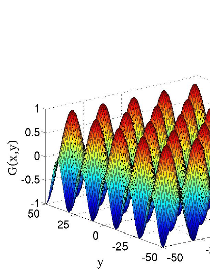
A B

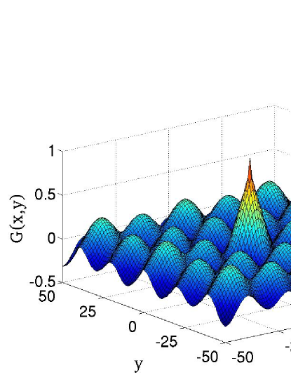
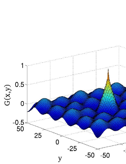
C D

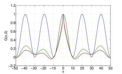
Figure 5: (Color online.) The correlator $G(x,y)$ for a two dimensional Screened Coulomb Ferromagnet of size 100 by 100. $J=1$, $Q=0.0004$, Screening length$=100\sqrt{2}$. A: $\mu=\mu_{min}=-0.0874$, B: $\mu=\mu_{min}+0.001$, C: $\mu=\mu_{min}+0.003$, D: G(x,y) for $y=0$ for A(blue)[$L_{D}=20$], B(green)[$L_{D}=24$] and C(red)[$L_{D}=26$].

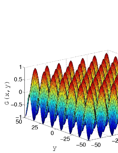
A B

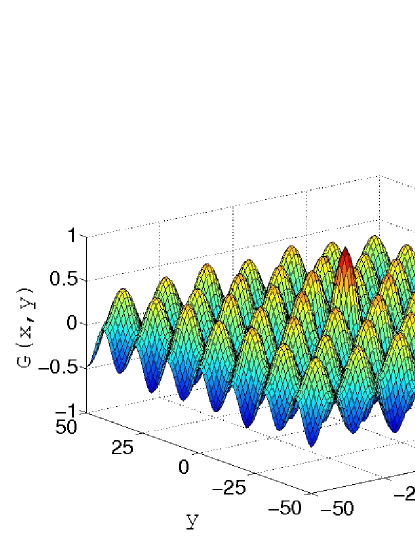
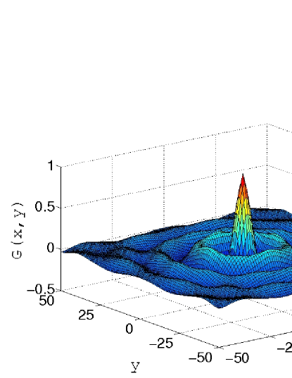
C D

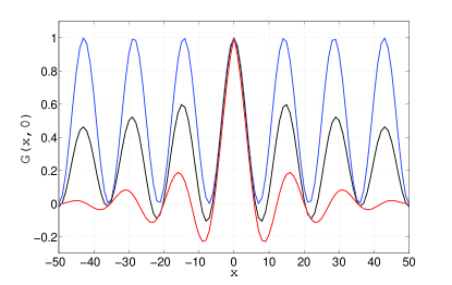
Figure 6: (Color online.) The correlator $G(x,y)$ for a two dimensional Dipolar Ferromagnet of size 100 by 100. $J=1$, $Q=0.15$. A: $\mu=\mu_{min}=-1.1459$, B: $\mu=\mu_{min}+4\times 10^{-5}$, C: $\mu=\mu_{min}+1\times 10^{-3}$, D: G(x,y) for $y=0$ for A(blue)[$L_{D}=14$], B(green)[$L_{D}=15$] and C(red)[$L_{D}=16$].

VI.2 Coexisting short range and screened Coulomb interactions

In this section, we study the screened Coulomb frustrated ferromagnet in more details. In the continuum limit, the Fourier transform of the interaction kernel of Eq.(5) with $V_{L}(x)$ given by Eq.(6) is

$$v(k)=Jk^{2}+\frac{Q}{k^{2}+\lambda^{2}}.$$ (71)

In appendix C, we provide explicit expressions for the dependence of $\mu$ on the temperature $T$. This dependence delineates the different temperature regimes. For $T>T^{*}$ wherein the temperature $T^{*}$ is set by

$$\mu(T^{*})=J\lambda^{2}+2\sqrt{JQ},$$ (72)

from Eq.(19), the pair correlator in $d=3$ dimensions is given by

$$G(\vec{x})=\frac{k_{B}T}{4\pi J|\vec{x}|}\frac{1}{\beta^{2}-\alpha^{2}}$$

$$\times[e^{-\alpha|\vec{x}|}(\lambda^{2}-\alpha^{2})-e^{-\beta|\vec{x}|}(\lambda^{2}-\beta^{2})].$$ (73)

Here,

$$\alpha^{2},\beta^{2}=\frac{\lambda^{2}+\mu/J\mp\sqrt{(\lambda^{2}-\mu/J)^{2}-4Q/J}}{2}.$$ (74)

By contrast, for temperatures $T<T^{*}$, we obtain an analytic continuation of Eq.(73) to complex $\alpha$ and $\beta$,

$$G(\vec{x})=\frac{k_{B}T}{8\alpha_{1}\alpha_{2}\pi J|\vec{x}|}e^{-\alpha_{1}|\vec{x}|}$$

$$\times[(\lambda^{2}-\alpha_{1}^{2}+\alpha_{2}^{2})\sin\alpha_{2}|\vec{x}|+2\alpha_{1}\alpha_{2}\cos\alpha_{2}|\vec{x}|],$$ (75)

In Eq.(75), $\alpha=\alpha_{1}+i\alpha_{2}=\beta^{*}$. In a similar fashion, in $d=2$ spatial dimensions, for $T>T^{*}$,

$$G(\vec{x})=\frac{k_{B}T}{2\pi}\frac{1}{\beta^{2}-\alpha^{2}}[(\lambda^{2}-\alpha^{2})K_{0}(\alpha|\vec{x}|)$$

$$+(\beta^{2}-\lambda^{2})K_{0}(\beta|\vec{x}|)].$$ (76)

As in the three dimensional case, the high temperature correlator of Eq.(76) may be analytically continued to lower temperatures, $T<T^{*}$, for which $\alpha$ and $\beta$ become complex.

High temperature limit

In the high temperature limit, in two spatial dimensions, from Eq.(76), we have,

$$G(\vec{x})=\frac{k_{B}T}{2\pi J}K_{0}\left(\sqrt{\frac{k_{B}T\Lambda^{2}}{4\pi J}}|\vec{x}|\right)-\frac{8\pi}{k_{B}T\Lambda^{4}}K_{0}\left(\lambda|\vec{x}|\right).$$

In three spatial dimensions, from Eq.(73), we have,

$$G(\vec{x})=\frac{k_{B}T}{4\pi J|\vec{x}|}e^{-\sqrt{\frac{k_{B}T\Lambda^{3}}{6\pi^{2}J}}|\vec{x}|}-\frac{9\pi^{3}Q}{k_{B}T\Lambda^{6}|\vec{x}|}e^{-\lambda|\vec{x}|}.$$ (78)

In the unscreened case, in two spatial dimensions,

$$G(\vec{x}) = \frac{k_{B}T}{2\pi J}K_{0}\left(\sqrt{\frac{k_{B}T\Lambda^{2}}{4\pi J}}|\vec{x}|\right)$$ (79)

$$-\frac{8\pi}{k_{B}T\Lambda^{4}}K_{0}\left(\sqrt{\frac{4\pi Q}{k_{B}T\Lambda^{2}}}|\vec{x}|\right).$$

In three spatial dimensions,

$$G(\vec{x}) = \Big{[}\frac{k_{B}T}{4\pi J|\vec{x}|}e^{-\sqrt{\frac{k_{B}T\Lambda^{3}}{6\pi^{2}J}}|\vec{x}|}$$ (80)

$$- \frac{9\pi^{3}Q}{k_{B}T\Lambda^{6}|\vec{x}|}e^{-\sqrt{\frac{6\pi^{2}Q}{k_{B}T\Lambda^{3}}}|\vec{x}|}\Big{]}.$$

From the above expressions, it is clear that the coefficients of the terms corresponding to the diverging correlation length goes to zero in the high temperature limit.

We note that two correlation lengths are manifest for all $(\mu-J\lambda^{2})^{2}>4JQ$. This includes all unfrustrated screened attractive Coulomb ferromagnets (those with $Q<0$)). The evolution of the correlation functions may be traced by examining the dynamics of the poles in the complex $k$ plane as a function of temperature. At high temperatures, correlations are borne by poles that lie on the imaginary $k$ axis.

Thermal evolution of modulation length at low temperatures

At $T=T^{*}$, the poles merge in pairs at $k=\pm i\sqrt{\lambda^{2}+\sqrt{Q/J}}$. At lower temperatures, $T<T^{*}$, the poles move off the imaginary axis (leading in turn to oscillations in the correlation functions). The norm of the poles, $|\alpha|=(Q/J+\lambda^{2}\mu(T)/J)^{1/4}$ tends to a constant in the limit of vanishing screening ($\lambda^{-1}=0$) wherein the after merging at $T=T^{*}$, the poles slide along a circle [Fig. 7]. In the low temperature limit of the unscreened Coulomb ferromagnet, the poles hit the real axis at finite $k$, reflecting oscillatory modulations in the ground state. In the presence of screening, the pole trajectories are slightly skewed [Fig. 8] yet for $Q/J>\lambda^{4}$, $\alpha$ tends to the ground state modulation wavenumber $\sqrt{\sqrt{Q/J}-\lambda^{2}}$. If the screening is sufficiently large, i.e., if the screening length is shorter than the natural period favored by a balance between the unscreened Coulomb interaction and the nearest neighbor attraction ($\lambda>(Q/J)^{1/4}$), then the correlation functions never exhibit oscillations. In such instances, the poles continuously stay on the imaginary axis and, at low temperatures, one pair of poles veers towards $k=0$ reflecting the uniform ground state of the heavily screened system.

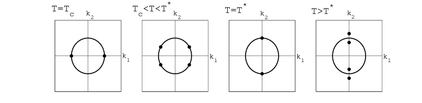
Figure 7: Location of the poles with increasing temperature (left to right) in the complex k-plane for the Coulomb frustrated ferromagnet. For temperatures below $T_{c}$, all the poles are real. Above $T_{c}$, the poles split in opposite directions of the real axis to give rise to two new complex poles. For $T_{c}<T<T^{*}$, we have complex poles. At $T^{*}$, pairs of such poles meet on the imaginary axis. Above $T^{*}$, the poles split along the imaginary axis. Thus, above $T^{*}$, the poles are purely imaginary.

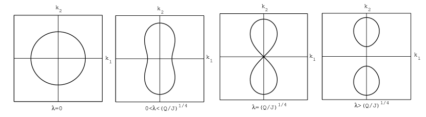
Figure 8: Trajectory of the poles in the complex $k$-plane for $T_{c}<T<T^{*}$ for the screened Coulomb ferromagnet. The screening length, $\lambda^{-1}$ decreases from left to right. In the first figure $\lambda=0$ and $\lambda>(Q/J)^{1/4}$ in the last figure.

To summarize, at high temperatures the pair correlator $G(x)$ is a sum of two decaying exponentials (one of which has a correlation length which diverges in the high temperature limit). For $T<T^{*}$ in under-screened systems, one of the correlation lengths turns into a modulation length characterizing low temperature oscillations. At the cross-over temperature $T^{*}$, the modulation length is infinite. As the temperature is progressively lowered, the modulation length decreases in size – until it reaches its ground state value. The temperature $T^{*}(Q/J,\lambda)$ is a “disorder line” dis like temperature [Fig 9].

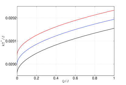
Figure 9: (Color online.) Temperature at which the modulation length diverges for a $100\times 100$ Coulomb frustrated ferromagnet plotted versus the relative strength of the Coulomb interaction with respect to the ferromagnetic interaction. [Blue:$\lambda=\lambda_{0}=1/(100\sqrt{2})$; Red:$\lambda=0.999\lambda_{0}$; Black:$\lambda=1.001\lambda_{0}$]

An analytical thermodynamic crossover does occur at $T=T^{*}$. A large $n$ calculation illustrates that the internal energy per particle

$$\frac{U}{N}=\frac{1}{2}(k_{B}T-\mu),$$ (81)

To detect a crossover in $U$ and that in other thermodynamic functions, the forms of $\mu$ both above and below $T^{*}$ may be derived from the spherical model normalization condition to find that the real valued functional form of $\mu(T)$ changes [See appendix C].

The system starts to exhibit order at the critical temperature $T=T_{c}$ given by

$$\frac{1}{k_{B}T_{c}}=\int\frac{d^{d}k}{(2\pi)^{d}}\frac{1}{v(\vec{k})-v(\vec{q})}.$$ (82)

For $Q/J>\lambda^{4}$, the modulus of the minimizing (ground state) wavenumber ($|\vec{q}|$) is given by

$$q=\frac{2\pi}{L_{D}^{g}}=\sqrt{\sqrt{Q/J}-\lambda^{2}},$$ (83)

with $L_{D}^{g}$ the ground state modulation length. Associated with this wavenumber is the kernel $v(\vec{q})=2\sqrt{JQ}-J\lambda^{2}$ to be inserted in Eq.(82) for an evaluation of the critical temperature $T_{c}$. Similarly, the ground state wavenumber $\vec{q}=0$ whenever $Q/J<\lambda^{4}$. If $Q/J>\lambda^{4}$ and modulations transpire for temperatures $T<T^{*}$, the critical temperature at which the chemical potential of Eq.(20), $\mu(T_{c})=J\lambda^{2}-2\sqrt{JQ}$, is lower than the crossover temperature $T^{*}$ (given by Eq.(72)) at which modulations first start to appear. The Screened Coulomb Ferromagnet has $T_{c}(Q/J=\lambda^{4})>0\mbox{ in $d>4$ dimensions}$ and in any dimension $T_{c}(Q/J>\lambda^{4})=0$. For small finite $n$, a first order Brazovskii transition may replace the continuous transition occurring at $T_{c}$ within the large $n$ limit Bra . Depending on parameter values such an equilibrium transition may or may not transpire before a possible glass transition may occur pet .

Domain length scaling in the Coulomb Frustrated Ferromagnet

The characteristic length-scales are governed by the position of the poles of $[v(k)+\mu]^{-1}$. See Fig. 7 for an illustration of the pole locations at low temperatures. For the frustrated Coulomb ferromagnet of Eq.(71) in the absence of screening ($\lambda^{-1}=0$),

$$v(k)+\mu=\frac{J}{k^{2}}(k^{4}+\frac{\mu}{J}k^{2}+\frac{Q}{J}).$$ (84)

Eq.(84) enable us to determine, in our large $n$ analysis, the cross-over temperature $T^{*}$ at which $\mu^{*}=\mu(T^{*})=2\sqrt{JQ}$. At $T=T^{*}$, the poles lie on the imaginary axis in $k$-plane. As the temperature is lowered below $T^{*}$, the two poles bifurcate. This bifurcation gives rise to finite size spatial modulations. At temperatures $T<T^{*}$, the four poles slide along a circle of fixed radius of size $(Q/J)^{1/4}$ (see Fig. 7). At zero temperature, these four poles merge in pairs to form two poles that lie on the real axis. The inverse modulation length is set by the absolute values of the real parts of the poles. We will set $\mu\equiv(2\sqrt{JQ}-\delta\mu)$. In the following, we will obtain the dependence of the real part of the poles on $\delta\mu$. The poles of $1/(v(k)+\mu)$ are determined by

$$k_{pole}^{2}=-\frac{\mu}{2J}\pm i\sqrt{\frac{Q}{J}-\frac{\mu^{2}}{4J^{2}}}=\sqrt{\frac{Q}{J}}e^{\pm 2i\theta}.$$ (85)

At $\mu=\mu^{*}$, the angle $\theta=\pi/2$. This point corresponds to the transition between (i) the high temperature region ($T>T^{*}$) wherein the system does not exhibit any modulations and (ii) the low temperature region ($T<T^{*}$). [See Fig. 7.] Eq.(85) implies that $\cos 2\theta=[1-\frac{\delta\mu}{\mu*}]$ or

$$k_{pole,real}=\frac{\delta\mu^{1/2}}{2J^{1/2}}.$$ (86)

Thus, we get a crossover exponent of $1/2$.

VI.3 Full direction and location dependent dipole-dipole interactions

In this subsection and the next, we consider systems where the spins are three dimensional and the interactions have the appropriate directional dependence. In this subsection, we will consider the effect of including the full dipolar interactions vis a vis the more commonly used scalar product form between two dipoles that is pertinent to two dimensional realizations. The dipolar interaction is given by

$$H_{dip}=\sum_{\vec{x}\neq\vec{y}}\left[\frac{\vec{S}(\vec{x})\cdot\vec{S}(\vec{y})}{r^{3}}-\frac{3[\vec{S}(\vec{x})\cdot\vec{r}][\vec{S}(\vec{y})\cdot\vec{r}]}{r^{5}}\right].$$ (87)

The two point correlator for a ferromagnetic system frustrated by this interaction is given, in the large $n$ approximation, by

$$G(\vec{x})=k_{B}T\int\frac{d^{d}k}{(2\pi)^{d}}e^{i\vec{k}\cdot\vec{x}}\left[\frac{2}{J\Delta(\vec{k})+Qv_{d}(k)+\mu}+\right.$$

$$\left.\frac{1}{J\Delta(\vec{k})-2Qv_{d}(k)+\mu}\right],$$ (88)

where $v_{d}(k)$ is given by Eqs.(69,70). For temperatures $T\leq T_{c}$,

$$\mu_{min}=-\min_{k\in\mathbb{R}}\{J\Delta(\vec{k})+Qv_{d}(k),$$

$$J\Delta(\vec{k})-2Qv_{d}(k)\}.$$ (89)

The Fourier transformed dipolar interaction kernel is positive definite, $v_{d}(k)>0$. An unscreened dipolar interaction leads to a $v_{d}(k)$ that diverges (tends to negative infinity) at its minimum at $k=0$. In the presence of both upper and lower distance cutoffs (see, e.g., Eq.(8) for a lower cutoff) on the dipolar interaction, the minimum of $v_{d}(k)$ attains a finite value and the system has a finite critical temperature.

Examining Eq.(88), we see that the introduction of the angular dependence in the dipolar interaction changes the results that would be obtained if the angular dependence were not included in a dramatic way.

(i) New correlation and modulation lengths arise from the second term in Eq.(88).

(ii) At low temperatures, the second term in Eq.(88) becomes dominant as its poles have a smaller real part (and thus a larger correlation length) relative to the first term in Eq.(88) that appears for an isotropic dipole-dipole interactions.

VI.4 Dzyaloshinsky- Moriya Interactions

As another example of a system with interactions having non-trivial directional dependence, we consider a system of three component spins with the Dzyaloshinsky-Moriya interaction D-M present along with the ferromagnetic interaction and a long range interaction,

$$H=-J\sum_{\langle\vec{x},\vec{y}\rangle}\vec{S}(\vec{x})\cdot\vec{S}(\vec{y})+\sum_{\langle\vec{x},\vec{y}\rangle}\vec{D}\cdot[\vec{S}(\vec{x})\times\vec{S}(\vec{y})]$$

$$+Q\sum_{\vec{x}\neq\vec{y}}V_{L}(|\vec{x}-\vec{y}|)\vec{S}(\vec{x})\cdot\vec{S}(\vec{y}).$$ (90)

We diagonalize this interaction kernel to obtain a Hamiltonian of the form,

$$H=\sum_{\vec{x},\vec{y}}\sum_{a}\hat{S}^{*}_{a}(\vec{x})V_{a}(\vec{x},\vec{y})\hat{S}_{a}(\vec{y}).$$ (91)

The $\hat{S_{a}}$’s are linear combinations of the components of $\vec{S}$. In a large $n$ approximation, the two point correlator is given by

$$G(\vec{x})=k_{B}T\int\frac{d^{d}k}{(2\pi)^{d}}e^{i\vec{k}\cdot\vec{x}}\left[\frac{1}{J\Delta(\vec{k})+Qv_{L}(k)+\mu}+\right.$$

$$\left.\frac{2(J\Delta(\vec{k})+Qv_{L}(k)+\mu)}{(J\Delta(\vec{k})+Qv_{L}(k)+\mu)^{2}+(D_{1}^{2}+D_{2}^{2}+D_{3}^{2})[\Delta(\vec{k})]^{2}}\right].$$ (92)

The presence of the Dzyaloshinsky-Moriya interaction does not alter the original poles and hence does not change the original length-scales of the system. However, additional length-scales arise due to the second term in Eq.(92).

A system of prominence where Dzyaloshinsky-Moriya interactions are important is MnSi DMJ . The spiral order is naturally susceptible to glass like dynamics. new ; DMJ

VII Conclusions

1. We studied the evolution of the ground state modulation lengths in frustrated Ising systems.

2. We investigated, in large $n$ theories, the evolution of modulation and correlation lengths as a function of temperature in different classes of systems.

3. We proved that, in large $n$ theories, the combined sum of the number of correlation and the number of modulation lengths is conserved. We have also showed that there exists a diverging modulation length at high temperatures for systems with long range interactions.

4. We studied three dimensional dipolar systems. We found that the full dipolar interactions with angular dependence included, changes the ground state of the system and also adds new length-scales.

It is a pleasure to acknowledge many discussions with Lincoln Chayes, Daniel Kivelson, Steven Kivelson, Michael Ogilvie, Joseph Rudnick, Gilles Tarjus, and Peter Wolynes. We also thank the Center for Materials Innovation – Washington University in St. Louis for providing partial financial support for this project.

Appendix A Transfer Matrix in the one-dimensional system with Ising spins

Thus far, we focused primarily on high dimensional continuous (large $n$) spin systems. For completeness, we review and illustrate how some similar conclusions can be drawn for one dimensional Ising systems with finite ranged interactions and briefly discuss trivial generalizations. In particular, we show how the sum of the number of modulation and number of correlation lengths does not change as the temperature is varied. In Section(V.3.3), we illustrated how this arises for general large $n$ systems.

For interactions of range $R$ in a one dimensional Ising spin chain, the transfer matrix, $T$ is of dimension $M={\cal{O}}(2^{R})$. The correlation function for large system size, takes the form

$$G(x)=\sum_{k=1}^{2^{R}-1}A_{k}\left(\frac{\lambda_{k}}{\lambda_{0}}\right)^{x},$$ (93)

where $\lambda_{i}$s are the eigenvalues of the transfer matrix. Since the characteristic equation has real non-negative coefficients, from Perron-Frobenius theorem, $\lambda_{0}$ is real, positive and is non-degenerate. The secular equation, $\det(T-\lambda I)=0$ is a polynomial in $\lambda$ with real coefficients. Thus, two possibilities need to be examined: real roots, and, complex conjugate pairs of roots. Real eigenvalues $\lambda_{p}$ give terms with correlation length,

$$\xi=\ln\left(\frac{\lambda_{0}}{|\lambda_{p}|}\right).$$ (94)

Complex conjugate eigenvalues, $\lambda_{q}$ and $\lambda_{q}^{*}$ correspond to the same correlation length and modulation length, given by,

$$\xi=\ln\left(\frac{\lambda_{0}}{|\lambda_{q}|}\right),$$ (95)

$$L_{D}=\frac{2\pi}{\tan^{-1}\left(\frac{\mbox{Im}\{\lambda_{q}\}}{\mbox{Re}\{\lambda_{q}\}}\right)}.$$ (96)

Thus, the total number of correlation and modulation lengths is the order of the polynomial in $\lambda$ in the secular equation, or simply the dimension of the transfer matrix – ${\cal{O}}(2^{R})$. Similar to our conclusions for the high dimensional continuous spin systems, this number does not vary with temperature. For $q$ state Potts type spins, replicating the above arguments mutatis mutandis, we find that the total number of correlation and modulation lengths is ${\cal{O}}(q^{R})$. Similarly, for such a system placed on a $d$ dimensional slab of finite extent in, at least, $(d-1)$ directions along which it has a length of order ${\cal{O}}(l)>R$, there will be ${\cal{O}}(q^{l^{d-1}})$ transfer matrix eigenvalues and thus an identical number for the sum of the number of modulation lengths with the number of correlation lengths.

The eigenvalues change from being complex below certain crossover temperatures to being purely real above. These temperatures form the “disorder line”.

Appendix B Detailed expressions for $\delta L_{D}$ for different orders $p(\geq 3)$ at which the interaction kernel has its first non-vanishing derivative

If the lowest order (larger than $p=2$) non-vanishing derivative of $v(k)$ at the minimizing wavenumber $k_{0}$ (see Eq.(33)) is of order $p=3$ (the most common case) then, in the large $n$ limit, the change in the modulation length at temperatures $T>T_{c}$ ($\mu(T)=\mu_{min}+\delta\mu$)about its value at $T=T_{c}$ of Eq.(43) is given by

$$\delta L_{D}=-\frac{2\pi}{k_{0}^{2}}\frac{v^{(3)}(k_{0})\delta\mu}{3(v^{(2)}(k_{0}))^{2}}.$$ (97)

We employ Eq.(97) in our analysis in Section(VI). If the lowest order derivatives are of order $p=4$ or $5$ then,

$$\delta L_{D}=\frac{2\pi}{k_{0}^{2}}\frac{v^{(5)}(k_{0})(\delta\mu)^{2}}{30(v^{(2)}(k_{0}))^{3}}.$$ (98)

Similarly, for $p=6$ or $7$,

$$\delta L_{D}=-\frac{2\pi}{k_{0}^{2}}\frac{v^{(7)}(k_{0})(\delta\mu)^{3}}{630(v^{(2)}(k_{0}))^{4}},$$ (99)

and so on.

Appendix C $\mu(T)$ for the screened Coulomb ferromagnet

We now briefly provide an explicit expression for the relation between the large $n$ Lagrange multiplier $\mu$ and the temperature $T$ for the screened Coulomb ferromagnet. In three dimensions, with $\Lambda$ as an ultra-violet cutoff, at high temperatures [$T>T^{*}$], we get to the following implicit equation for $\mu(T)$ in the case of the screened Coulomb ferromagnet of Eq.(71),

$$\frac{1}{T}=\frac{\Lambda}{2\pi^{2}}+\frac{\sqrt{2}}{4\pi^{2}p}$$

$$\times\Big{(}\frac{\lambda^{2}\mu-\mu^{2}+\mu p-2Q}{\sqrt{\lambda^{2}+\mu+p}}\tan^{-1}(\frac{\Lambda\sqrt{2}}{\sqrt{\lambda^{2}+\mu+p}})$$

$$-\frac{\lambda^{2}\mu-\mu^{2}+\mu p+2Q}{\sqrt{\lambda^{2}+\mu-p}}\tan^{-1}(\frac{\Lambda\sqrt{2}}{\sqrt{\lambda^{2}+\mu-p}})\Big{)}.$$ (100)

In Eq.(100), we employed the shorthand $p\equiv\sqrt{(\mu-\lambda^{2})^{2}-4Q}$. The parameter $p$ vanishes at the crossover temperature $T^{*}$ at which a divergent modulation length makes an appearance, $p(T=T^{*})=0$. At low temperatures, $T<T^{*}$, $p$ becomes imaginary and an analytical crossover occurs to another real functional form.

Appendix D Proof that $\mu(T)$ is an analytic function of $T$

In this appendix, we illustrate that in the large $n$ limit, the thermodynamic functions are analytic for all temperatures $T>T_{c}$, including the discussed cross-over temperature $T=T^{*}$ (hence justifying the use of the term ”cross-over”) of, e.g, the Coulomb frustrated ferromagnet of Eqs.(1, 71).

From Eq. (21), using,

$$\mu>\mu_{\min}=-\min{v(k)},$$ (101)

it is clear that $\mu(T)$ is a continuous function of $T$. Differentiating,

$$\frac{d\mu}{d(k_{B}T)}=\left[(k_{B}T)^{2}\int\frac{d^{d}k}{(v(k)+\mu)^{2}}\right]^{-1},$$ (102)

and,

$$\frac{d^{2}\mu}{d(k_{B}T)^{2}}=-\frac{2}{k_{B}T}\frac{d\mu}{d(k_{B}T)}+$$

$$2(k_{B}T)^{2}\left(\frac{d\mu}{d(k_{B}T)}\right)^{3}\int\frac{d^{d}k}{(v(k)+\mu)^{3}}$$ (103)

with the integrations performed over the first Brillouin zone on the lattice (or up to some ultra-violet cutoff $\Lambda$ in the continuum). The first two derivatives are thus always finite so long as the integration range is finite. All higher order derivatives are sum of terms which are products of lower order derivatives, $(k_{B}T)^{a}$ and $\int\frac{d^{d}k}{(v(k)+\mu)^{b}}$, where $a$ and $b$ are integers, with $b>0$. Thus, for finite integration range, $\mu(T)$ is an analytic function of $T$. In the large $n$ limit, the internal energy per site, $U/N=[k_{B}T-\mu(T)]/2$. Our result concerning the analyticity of $\mu(T)$ implies that the internal energy is analytic and thus all of its derivatives and all other thermodynamic potentials.

References

- (1) E. Ising, Zeits. f. Physik. 31, 253 (1925).
- (2) T. Dauxios, S. Ruffo, E. Arimondo, M. Wilkens (Eds.), “Dynamics and Thermodynamics of Systems with Long Range Interactions”, Lecture Notes in Physics 602, Springer (2002).
- (3) A. Giuliani, J. L. Lebowitz and E. H. Lieb, Phys. Rev. B 76, 184426 (2007); A. Giuliani, J. L. Lebowitz and E. H. Lieb, Phys. Rev. B 74, 064420 (2006).
- (4) A. Vindigni, N. Saratz, O. Portmann, D. Pescia, and P. Politi, Phys. Rev. B 77, 092414 (2008).
- (5) C. Ortix, J. Lorenzana, and C. Di Castro, Phys. Rev. B 73, 245117 (2006).
- (6) I. Daruka and Z. Gulácsi, Phys. Rev. E 58, 5403 (1998).
- bar (a) D. G. Barci and D. A. Stariolo, Phys. Rev. B 79, 075437 (2009).
- (8) M. M. Fogler, arXiv:cond-mat/0111001, p. 98-138, in High Magnetic Fields: Applications in Condensed Matter Physics and Spectroscopy, ed. by C. Berthier, L.-P. Levy, G. Martinez (Springer-Verlag, Berlin, 2002).
- (9) Hyung-June Woo, C. Carraro, D. Chandler, Phys. Rev. E 52, 6497 (1995); F. Stilinger, J. Chem. Phys. 78, 4655 (1983); L. Leibler, Macromolecules 13, 1602 (1980); T. Ohta and K. Kawasaki, Macromolecules 19, 2621 (1986).
- vor (a) H. Kleinert, “Gauge Fields in Condensed Matter”, World Scientific (1989), volume II .
- vor (b) P. H. Chavanis, “Statistical Mechanics of Two Dimensional Vortices and Stellar systems” in Ref.[lon ].
- vor (c) H. Kleinert, “Gauge Fields in Condensed Matter”, World Scientific (1989), volume I .
- (13) M. Seul and D. Andelman, Science 267, 476 (1995).
- (14) Y. Elskens, “Kinetic Theory for Plasmas and Wave-particle Hamiltonian Dynamics”, in lon ; Y. Elskens and D. Escande, “Microscopic Dynamics of Plasmas and Chaos”, IOP publishing, Bristol (2002).
- (15) V. J. Emery and S. A. Kivelson, Physica C 209, 597 (1993).
- (16) L. Chayes, V. J. Emery, S. A. Kivelson, Z. Nussinov, and G. Tarjus, Physica A 225, 129 (1996).
- zoh (a) Z. Nussinov , J. Rudnick, S. A. Kivelson, and L. N. Chayes, Phys. Rev. Letters 83, 472 (1999).
- Löw et al. (1994) U. Löw, V. J. Emery, K. Fabricius, and S. A. Kivelson, Phys. Rev. Lett. 72, 1918 (1994).
- (19) E. W. Carlson, V. J. Emery, S. A. Kivelson, D. Orgad, “Concepts in High Temperature Superconductivity” in “The Physics of Superconductors” ed. K.H. Bennemann and J.B. Ketterson (Springer-Verlag 2004), 180 pages. See also arXiv:cond-mat/0206217.
- (20) V.B. Nascimento et. al., arXiv:0905.3194.
- (21) S- W. Cheong et al., Phys. Rev. Lett. 67, 1791 (1991).
- (22) D. I. Golosov, Phys. Rev. B, vol. 67, 064404 (2003). (arXiv:cond-mat/0206257).
- Kivelson et al. (1995) D. Kivelson, S. A. Kivelson, X. Zhao, Z. Nussinov, and G. Tarjus, Physica A: Statistical and Theoretical Physics 219, 27 (1995), ISSN 0378-4371.
- (24) J. Schmalian and P. G. Wolynes, Phys. Rev. Lett. 85, 836 (2000); H. Westfahl, Jr., J. Schmalian, and P. G. Wolynes, Phys. Rev. B 64, 174203 (2001).
- (25) G. Tarjus, S. A. Kivelson, Z. Nussinov and P. Viot, J. Phys Cond. Matt. 17, 50 (2005).
- (26) Z. Nussinov, Phys. Rev. B 69, 014208 (2004).
- (27) G. Tarjus, S. A. Kivelson, Z. Nussinov, and P. Viot, J. Phys: Condens. Matter 17, R1143 (2005).
- (28) B. V. Derjaguin and L. Landau, Acta Physiochim, URSS 14, 633 (1941); E. J. Verwey and J. T. G. Overbeek Theory of Stability of Lyophobic Colloids (Elsevier, Amsterdam, 1948).
- (29) C. Reichhardt and C. J. Olson, Phys. Rev. Lett. 88, 248301 (2002).
- bar (b) J. Barre, D. Mukamel, S. Ruffo, “Ensemble inequivalence in mean field models of magnetism” in lon .
- (31) Mark Ya. Azbel Phys. Rev. E 68, 050901 (2003).
- zoh (b) Z. Nussinov, arXiv:cond-mat/0105253 (2001) – in particular, see footnote [20] therein for the Ising ground states.
- (33) T. H. Berlin and M. Kac, Phys. Rev. 86, 821 (1952).
- Stanley (1968) H. E. Stanley, Phys. Rev. 176, 718 (1968).
- (35) J. Stephenson, Phys. Rev B, 1, 4405 (1970); J. Stephenson, Can. J. Phys, 48, 1724 (1970); N. Alves Jr. and C. S. O. Yokoi, Braz. J. Phys., 30, 4 (2000); W. Selke, Phys. Rep., 170, 213 (1988).
- (36) S. Brazovskii, Sov. Phys. JETP 41, 85 (1975).
- (37) I. Dzyaloshinsky, J. Phys. Chem. Solids 4, 241 (1958); T. Moriya, Phys. Rev 120, 1, 91 (1960).
- (38) J. Schmalian and M. Turlakov, Phys. Rev. Lett. 93, 036405 (2004).