Semiclassical Wigner distribution for two-mode entangled state
generated by an optical parametric oscillator

Abstract

We derive the steady state solution of the Fokker-Planck equation that describes the dynamics of the nondegenerate optical parametric oscillator in the truncated Wigner representation of the density operator. The adiabatic limit of strong pump damping is assumed. This phase space image provides a clear view of the intracavity two-mode entangled state valid in all operating regimes of the OPO. A nongaussian distribution is obtained for the above threshold solution.

I Introduction

Among the quasiprobability functions that represent the density operator of a quantum state, the Wigner distribution has undoubtedly advantages over others, since in this phase space representation the quantum-classical correspondence is, in general, much more visible. At the same time these functions contain all information available in the density operator.

Unfortunately, just a few states have been represented by this distribution due to the difficulty to solve Fokker-Planck equations for nonlinear systems. Indeed, the phase space description of quantum systems is well known for quadratic hamiltonians, but very little is known for nonlinear systems, such as, for example, the single-mode degenerate parametric oscillator kinsler , or the transverse multimode degenerate parametric oscillator kaled2 .

Of special interest is the two-mode entangled state generated in the optical parametric oscillator (OPO), used in many experiments of quantum information. The Wigner distribution of this state was obtained exactly using the solution derived from the complex P-representation karen , and tranformed into a Wigner distribution. Since this analytical result appears as an infinite series of gamma functions (hypergeometric series), some important physical aspects are hidden by its mathematical complexity. For example, two-mode entanglement is not of easy identification from the usual partial transpose criterion simon ; duan . The same happens to the generalized P-representation for the intracavity parametric oscillator derived in Ref.mcneil . In order to calculate the intensity correlations, the authors obtained an integral expression that depends on degenerate hypergeometric functions, and the outcome also depends on an infinite sum.

In the present work, we derive the Wigner function of a two-mode quantum state of the electromagnetic field generated by an OPO using a truncated Wigner equation. This truncated approximation is valid when the nonlinearity is small enough, which is true for most of the OPO experiments developed so far. A simple expression is obtained for the Wigner distribution, which renders clear the many quantum features of the intracavity OPO field such as squeezing and entanglement. Moreover, this expression is valid in all regions of the OPO operation regimes, that is, below, and above threshold, where the validity of both the linear approximation, and the perturbation theory break down. This distribution also describes the OPO quantum fluctuations properly around the operation threshold, while the usual linear approach provides divergent results. In order to illustrate the reliability of the Wigner function we obtain, moments calculated from this distribution are compared with the exact quantum results, for any values of the control parameters of the OPO.

II Theoretical model

We present here a model of three quantized modes coupled by a nonlinear crystal inside a triply resonant Fabry-Perot cavity. The Heisenberg picture Hamiltonian that describes this open system is given bycarmichael

$$\hat{H} = \sum_{i=0}^{2}\hbar\omega_{i}\hat{a}_{i}^{\dagger}\hat{a}_{i}+i\hbar\chi\left(\hat{a}_{1}^{\dagger}\hat{a}_{2}^{\dagger}\hat{a}_{0}-\hat{a}_{1}\hat{a}_{2}\hat{a}_{0}^{\dagger}\right)$$ (1)

$$+ i\hbar\left(Ee^{-i\omega_{0}t}\hat{a}_{0}^{\dagger}-E^{*}e^{i\omega_{0}t}\hat{a}_{0}\right)$$

$$+ \sum_{i=0}^{2}\left(\hat{a}_{i}\hat{\Gamma}_{i}^{\dagger}+\hat{a}_{i}^{\dagger}\hat{\Gamma}_{i}\right)\;.$$

Here $E$ represents the external coherent driving pump field at frequency $\omega_{0}$. The operators $\hat{a}_{0}$, $\hat{a}_{1}$ and $\hat{a}_{2}$ represent the pump, signal and idler fields, respectively, satisfying the following frequency matching condition, $\omega_{0}=\omega_{1}+\omega_{2}$. The terms $\hat{\Gamma}_{i}$ represent damping reservoir operators, and $\chi$ is the nonlinear coupling constant due to the second order polarizability of the nonlinear crystal.

The master equation for the reduced density operator, after the elimination of the heat bath by standard techniques carmichael , is given by

$$\frac{\partial\hat{\rho}}{\partial t} = -i\sum_{i=0}^{2}\omega_{i}\left[\hat{a}_{i}^{\dagger}\hat{a}_{i},\hat{\rho}\right]+\chi\left[\hat{a}_{1}^{\dagger}\hat{a}_{2}^{\dagger}\hat{a}_{0},\hat{\rho}\right]-\chi\left[\hat{a}_{1}\hat{a}_{2}\hat{a}_{0}^{\dagger},\hat{\rho}\right]$$ (2)

$$+Ee^{-i\omega_{0}t}\left[\hat{a}_{0}^{\dagger},\hat{\rho}\right]-E^{*}e^{i\omega_{0}t}\left[\hat{a}_{0},\hat{\rho}\right]$$

$$+\sum_{i=0}^{2}\gamma_{i}\left(2\hat{a}_{i}\hat{\rho}\hat{a}_{i}^{\dagger}-\hat{a}_{i}^{\dagger}\hat{a}_{i}\hat{\rho}-\hat{\rho}\hat{a}_{i}^{\dagger}\hat{a}_{i}\right)\;,$$

where $\gamma_{i}$ is the corresponding mode damping rate.

In order to treat the operators evolution, we now turn to the method of operator representation theory. These techniques can be used to transform the density matrix equation of motion into c-number Fokker-Planck or stochastic equations. We can write down the master equation in the Wigner representation, by using the following characteristic function

$$\chi_{W}(z,z^{*}) = Tr\left(\rho e^{iz^{*}a^{\dagger}+iza}\right)$$ (3)

$$= Tr\left(\rho e^{iz^{*}a^{\dagger}}e^{iza}e^{-|z|^{2}/2}\right)\;,$$

so that the Wigner distribution can be written as Fourier transform of the characteristic function:

$$W(\alpha,\alpha^{*})=\frac{1}{\pi^{2}}\int_{-\infty}^{\infty}d^{2}z\;\chi_{W}(z,z^{*})e^{-iz^{*}\alpha^{*}}e^{-iz\alpha}\;.$$ (4)

The phase space Wigner equation for the nondegenerate parametric amplifier that corresponds to the master equation (2) is then

$$\frac{\partial W}{\partial t} = \left\{\frac{\partial}{\partial\alpha_{0}}\left(i\omega_{0}\alpha_{0}+\gamma_{0}\alpha_{0}+\chi\alpha_{1}\alpha_{2}-Ee^{-i\omega_{0}t}\right)\right.$$ (5)

$$+ \frac{\partial}{\partial\alpha_{0}^{*}}\left(-i\omega_{0}\alpha_{0}^{*}+\gamma_{0}\alpha_{0}^{*}+\chi\alpha_{1}^{*}\alpha_{2}^{*}-E^{*}e^{i\omega_{0}t}\right)$$

$$+ \frac{\partial}{\partial\alpha_{1}}\left(i\omega_{1}\alpha_{1}+\gamma_{1}\alpha_{1}-\chi\alpha_{2}^{*}\alpha_{0}\right)$$

$$+ \frac{\partial}{\partial\alpha_{1}^{*}}\left(-i\omega_{1}\alpha_{1}^{*}+\gamma_{1}\alpha_{1}^{*}-\chi\alpha_{2}\alpha_{0}^{*}\right)$$

$$+ \frac{\partial}{\partial\alpha_{2}}\left(i\omega_{2}\alpha_{2}+\gamma_{2}\alpha_{2}-\chi\alpha_{1}^{*}\alpha_{0}\right)$$

$$+ \frac{\partial}{\partial\alpha_{2}^{*}}\left(-i\omega_{2}\alpha_{2}^{*}+\gamma_{2}\alpha_{2}^{*}-\chi\alpha_{1}\alpha_{0}^{*}\right)$$

$$+ \gamma_{0}\frac{\partial^{2}}{\partial\alpha_{0}\partial\alpha_{0}^{*}}+\gamma_{1}\frac{\partial^{2}}{\partial\alpha_{1}\partial\alpha_{1}^{*}}+\gamma_{2}\frac{\partial^{2}}{\partial\alpha_{2}\partial\alpha_{2}^{*}}$$

$$+ \left.\frac{\chi}{4}\left(\frac{\partial^{3}}{\partial\alpha_{1}\partial\alpha_{2}\partial\alpha_{0}^{*}}+\frac{\partial^{3}}{\partial\alpha_{1}^{*}\partial\alpha_{2}^{*}\partial\alpha_{0}}\right)\right\}W\;.$$

This is not a Fokker-Planck equation due to the third order derivative term, but in the case where $\chi$ is small enough we can drop this term. The truncated equation so obtained is a genuine Fokker-Planck equation with a positive diffusion term, and we can easily derive the corresponding stochastic differential equations in the rotating frame ($\tilde{\alpha}_{j}=\alpha_{j}\exp{(-i\omega_{j}t)}$ with $j=0,1,2$):

$$\frac{d\tilde{\alpha}_{0}}{dt}=-\gamma_{0}\tilde{\alpha}_{0}+E-\chi\tilde{\alpha}_{1}\tilde{\alpha}_{2}+\sqrt{\gamma_{0}}\xi_{0}(t)\;,$$

$$\frac{d\tilde{\alpha}_{1}}{dt}=-\gamma_{1}\tilde{\alpha}_{0}+\chi\tilde{\alpha}_{0}\tilde{\alpha}_{2}^{*}+\sqrt{\gamma_{1}}\xi_{1}(t)\;,$$

$$\frac{d\tilde{\alpha}_{2}}{dt}=-\gamma_{2}\tilde{\alpha}_{0}+\chi\tilde{\alpha}_{0}\tilde{\alpha}_{1}^{*}+\sqrt{\gamma_{2}}\xi_{2}(t)\;.$$ (6)

It is possible to find a stationary solution of the truncated Fokker-Planck equation when we adiabatically eliminate the pump mode variables. This means that we are considering the relaxation rate of this mode much larger than those of the downconverted modes, that is $\gamma_{0}\gg\gamma_{1},\gamma_{2}$. The stationary solution for the pumped mode is

$$\tilde{\alpha}_{0}=\frac{1}{\gamma_{0}}\left[E-\chi\tilde{\alpha}_{1}\tilde{\alpha}_{2}+\sqrt{\gamma_{0}}\xi_{0}(t)\right]\;,$$ (7)

where the noise term is retained in the adiabatic elimination in order to properly deal with the noise dynamics. We are then left with two nonlinear dynamical equations for the complex amplitudes of the down-converted fields, where the pump amplitude is replaced by expression (7).

We now define the following real quadrature variables:

$$x_{1}=\tilde{\alpha}_{1}+\tilde{\alpha}_{1}^{*}\;,\,\,\,\,\,\,\,\,\,\,y_{1}=-i\left(\tilde{\alpha}_{1}-\tilde{\alpha}_{1}^{*}\right)\;,$$

$$x_{2}=\tilde{\alpha}_{2}+\tilde{\alpha}_{2}^{*}\;,\,\,\,\,\,\,\,\,\,\,y_{2}=-i\left(\tilde{\alpha}_{2}-\tilde{\alpha}_{2}^{*}\right)\;,$$ (8)

so that the remaining dynamical equations can be cast in the compact form:

$$\frac{d\mathbf{X}}{dt}=\mathbf{A}+\mathbf{B}\,\mathbf{\xi}(t)$$ (9)

where $\mathbf{X}=[x_{1},y_{1},x_{2},y_{2}]^{T}$ is a column vector, and the drift matrix is defined as

$$\mathbf{A}=\gamma\left[\begin{array}[]{c}-x_{1}+\mu x_{2}-\frac{g^{2}}{2}x_{1}\left(x_{2}^{2}+y_{2}^{2}\right)\\ \vskip 6.0pt plus 2.0pt minus 2.0pt\cr-y_{1}-\mu y_{2}-\frac{g^{2}}{2}y_{1}\left(x_{2}^{2}+y_{2}^{2}\right)\\ \vskip 6.0pt plus 2.0pt minus 2.0pt\cr-x_{2}+\mu x_{1}-\frac{g^{2}}{2}x_{2}\left(x_{1}^{2}+y_{1}^{2}\right)\\ -y_{2}-\mu y_{1}-\frac{g^{2}}{2}y_{2}\left(x_{1}^{2}+y_{1}^{2}\right)\\ \end{array}\right]\;.$$ (10)

We have set $\gamma_{1}=\gamma_{2}=\gamma$, which is a reasonable physical assumption for most OPO experiments, and defined the normalized pump parameter $\mu=\chi E/(\gamma\gamma_{0})$, as well as the nonlinear coupling $g=\chi/(\sqrt{2\gamma\gamma_{0}})$. $\mathbf{B}$ is a $4\times 6$ matrix defined as

$$\mathbf{B}=\sqrt{2\gamma}\left(\begin{array}[]{cccccc}1&0&0&0&\frac{g}{\sqrt{2}}x_{2}&\frac{g}{\sqrt{2}}y_{2}\\ 0&1&0&0&-\frac{g}{\sqrt{2}}y_{2}&\frac{g}{\sqrt{2}}x_{2}\\ 0&0&1&0&\frac{g}{\sqrt{2}}x_{1}&\frac{g}{\sqrt{2}}y_{1}\\ 0&0&0&1&-\frac{g}{\sqrt{2}}y_{1}&\frac{g}{\sqrt{2}}x_{1}\\ \end{array}\right)$$ (11)

and ${\mathbf{\xi}}(t)$ is a six component column vector whose entries are uncorrelated real Gaussian noises associated with the noise terms for the three interacting fields.

Now this set of stochastic equations can be mapped onto a genuine Fokker-Planck equation:

$$\frac{\partial W(\mathbf{X})}{\partial t}=\left[-\frac{\partial}{\partial\mathbf{X}_{i}}\mathbf{A}_{i}+\frac{1}{2}\frac{\partial}{\partial\mathbf{X}_{i}}\frac{\partial}{\partial\mathbf{X}_{j}}\mathbf{D}_{ij}\right]W(\mathbf{X})$$ (12)

where the diffusion matrix is defined as $\mathbf{D}=\mathbf{B}\mathbf{B}^{T}$, and summation over repeated indices is assumed throughout the text.

This Fokker-Planck equation admits a steady state solution in the potential form $W(\mathbf{X})=N\exp{(-\int\mathbf{Z}_{i}\,d\mathbf{X}_{i})}$ with $\mathbf{Z}_{i}$ given by

$$\mathbf{Z}_{i}=\mathbf{D}_{ik}^{-1}\left[2\mathbf{A}_{k}-\frac{\partial}{\partial\mathbf{X}_{j}}\mathbf{D}_{ij}\right]\;.$$ (13)

This solution provides a quite simple form for the Wigner distribution which allows for the calculation of several statistical properties. It is important to notice that the potential solution is achievable only when $\gamma_{1}=\gamma_{2}\equiv\gamma$ as we have already assumed gardiner . In this case, the steady state Wigner distribution for signal and idler reads:

$$W(x_{1},y_{1},x_{2},y_{2})={\cal{N}}\exp\left\{\frac{-1/2}{1+\frac{g^{2}}{2}\left(x_{1}^{2}+y_{1}^{2}+x_{2}^{2}+y_{2}^{2}\right)}\right.$$

$$\times\left[\left(1+g^{2}\right)\left(x_{1}^{2}+y_{1}^{2}+x_{2}^{2}+y_{2}^{2}\right)+2\mu\left(y_{1}y_{2}-x_{1}x_{2}\right)\right.$$

$$+\left.\left.g^{2}\left(x_{1}^{2}+y_{1}^{2}\right)\left(x_{2}^{2}+y_{2}^{2}\right)\right]\right\}$$ (14)

where ${\cal{N}}$ is the normalization constant and unimportant terms $O(g^{4})$ were neglected in the argument of the potential solution.

As a concrete physical example, expression (14) can describe the joint Wigner distribution for two polarization modes of a frequency degenerate type II OPO, where signal and idler are distinguished by their polarization states. All statistical properties, including experimentally accessible quantities like quadrature noise and correlations in the stationary state may be calculated with this distribution in any OPO operation regime. It is interesting to notice that the distribution given by expression (14) is single peaked below threshold operation ($\mu<1$) and becomes double peaked above threshold. In Fig. (1), it is possibible to visualize the conditional Wigner distribution for fixed values of $y_{1}$ and $y_{2}$, for an OPO operating below, at, and above threshold. It is easy to identify the squeezed and unsqueezed quadratures in all regimes.

Figure 1: Conditional Wigner distribution for $y_{1}=0$ and $y_{2}=0$, a) below ($\mu=0.5$); b) at ($\mu=1.0$); and c) above threshold ($\mu=1.5$). In all cases $g^{2}=0.01$.

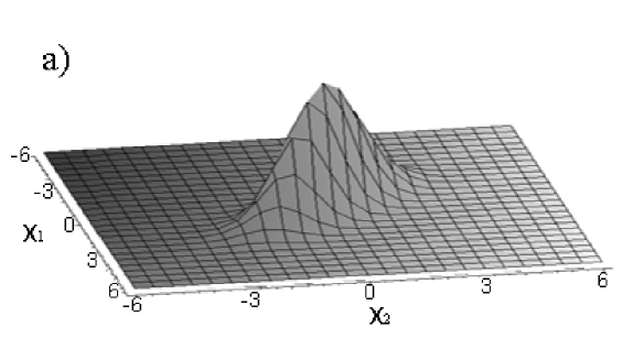
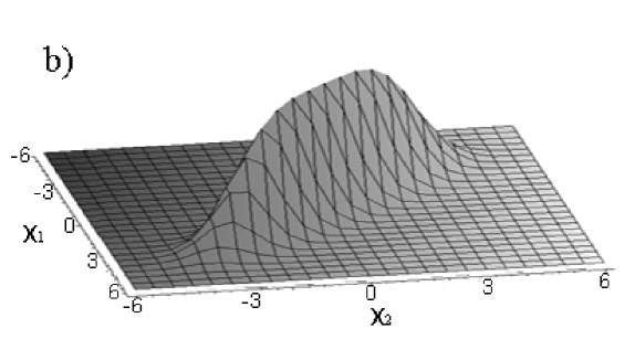
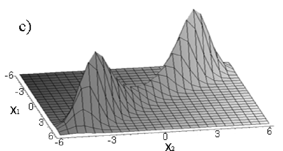
For the nonlinear media employed in most OPO devices, the coupling parameter $g\ll 1$. Therefore, the first two terms in the exponent of the Wigner distribution governs the OPO behaviour below threshold. They are enough to predict the usual nonclassical features. In fact, it is evident now that the usual linearized approach to quantum noise in below-threshold OPOs is equivalent to completely neglect the $g^{2}$ term in the distribution. However, it is important to notice that for $\mu\geq 1$, the Wigner distribution becomes divergent if we neglect the $g^{2}$ term. This means that this term plays a crucial role for a complete description of the OPO behaviour at and above threshold.

Additional insight is provided by a careful investigation of the marginal distribution obtained by integrating $W(x_{1},y_{1},x_{2},y_{2})$ with respect to one mode variables. Of course, due to the symmetry of $W$, the form of the resulting marginal distribution is independent of the mode being traced out. The marginal distribution for mode 2 becomes:

$$W\left(x_{2},y_{2}\right)=2\pi{\cal{N}}\times$$ (15)

$$\exp\left(\frac{-\left(x_{2}^{2}+y_{2}^{2}\right)\left(1+g^{2}\left(1+x_{2}^{2}+y_{2}^{2}\right)-\mu^{2}\right)}{2\left(1+g^{2}\left(x_{2}^{2}+y_{2}^{2}\right)\right)^{2}}\right)$$

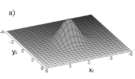
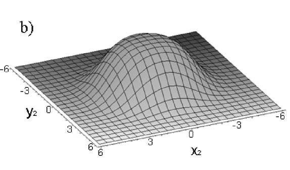
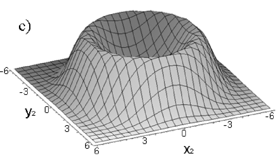
It gives the statistical properties of isolated measurements on mode 2. The variances given by this marginal distribution are larger than those of the vacuum state. This excess noise can be seen as a consequence of information loss when one looks only at part of the whole system. Fig. (2) presents the marginal distribution below, at and above threshold. Above threshold the marginal distribution is clearly peaked out of the phase space origin, what is a consequence of the macroscopic amplification of the down-converted fields. However, the distribution presents radial symmetry indicating complete phase uncertainty in each individual mode.

Figure 2: Marginal distributions: a) below threshold, $\mu=0.8$; b) at threshold, $\mu=1.0$; c) above threshold, $\mu=1.2$. In all cases $g^{2}=0.01$.

III Comparison with the linearized quantum approach

Almost the totality of theoretical works devoted to the analysis of quantum noise in optical systems rely on linearization of the small quantum fluctuations around the macroscopic steady state mean values. It is worth to notice that this procedure has limited validity, especially around the threshold critical point where quantum fluctuations may become comparable to the mean values. In order to evidence the breakdown of the linearized theory, we shall compare its results with those obtained from the solution of the Fokker-Planck equation (12).

The usual approach given to quantum noise in the literature is obtained from first order stochastic equations of motion kaled ; villar . These equations are often used to predict squeezing in a linearized fluctuation analysis. They are non-classical in the sense that they can describe states without a positive Glauber-Sudarshan P-distribution, but correspond to a Gaussian Wigner distribution.

We now find it useful to introduce combined field quadratures, as in two-mode approaches used previously Caves . These combined quadratures are the Einstein-Podolsky-Rosen (EPR) variables used to characterize continuous variable entanglement between the down converted fields. They are defined as

$$x_{\pm}=\frac{x_{1}\pm x_{2}}{\sqrt{2}},\;\;\;\;\;\;y_{\pm}=\frac{y_{1}\pm y_{2}}{\sqrt{2}}.$$ (16)

These quantities correspond to the squeezed and anti-squeezed combined quadratures obtained in the linearized theory. ¿From the first order stochastic equations one can easily obtain the steady state variances of the EPR variables kaled ; villar :

$$\langle x_{+}^{2}\rangle = \langle y_{-}^{2}\rangle=\frac{1}{1-\mu}$$

$$\langle x_{-}^{2}\rangle = \langle y_{+}^{2}\rangle=\frac{1}{1+\mu}$$ (17)

for below threshold operation, and

$$\langle x_{+}^{2}\rangle = \langle y_{-}^{2}\rangle=\frac{1}{\mu-1}+\frac{1}{g^{2}}(\mu-1)$$

$$\langle x_{-}^{2}\rangle = \langle y_{+}^{2}\rangle=\frac{1}{2}$$ (18)

for above threshold operation.

Now let us briefly discuss the predictions of the linearized approach and its validity. The quadratures $x_{-}$ and $y_{+}$ exhibit the expected squeezing, going from the vacuum fluctuations for zero pump until 50% intracavity squeezing (which corresponds to perfect squeezing outside the cavity) at and above the oscillation threshold. The unsqueezed quadratures $x_{+}$ and $y_{-}$ present divergent behaviour around threshold, which is certainly not physical. In fact, as we shall see next, the steady state solution of the Fokker-Planck equation (12) gives a well behaved Wigner distribution which does not display any divergences. This Wigner distribution will also put limits on the amount of squeezing attainable.

In order to investigate the two-mode entanglement directly from the Wigner distribution, we now write it in terms of the EPR variables. Below threshold, where the linearization of the equation of motion is valid, we can neglect the $g^{2}$ term, and the distribution can be approximated as

$$W_{L}(x_{+},y_{+},x_{-},y_{-})={\cal{N}}exp\left\{-\frac{1}{2}\left[\left(1+\mu\right)x_{-}^{2}+\right.\right.$$

$$\left.\left.\left(1+\mu\right)y_{+}^{2}+\left(1-\mu\right)x_{+}^{2}+\left(1-\mu\right)y_{-}^{2}\right]\right\}\;.$$ (19)

With this expression we can easily calculate any moment of the distribution. For instance, we easily reobtain the results of Eqs.(17) for the intracavity noise squeezing in the combined quadratures. As we mentioned before, at threshold we have perfect external squeezing while the unsqueezed combined quadratures blow up showing the failure of linearization kaled . Moreover, it is easy to characterize this state as entangled by using the Duan-Simon criterion simon ; duan . Above threshold we can also calculate the moments and we find that this criterion shows the suficient condition to characterize this state as entangled, in spite of not being a Gaussian state in that regime.

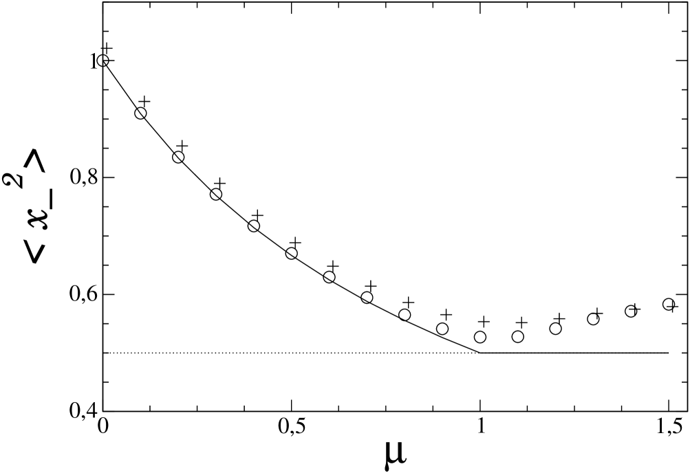
It is also interesting to compare the results obtained for $\langle x^{2}_{+}\rangle$ with the linearized theory (both below and above threshold) with those obtained from the Wigner function given by Eq.(14). This is done in Fig.(3). While the linearized approach gives a divergent behavior at the oscillation threshold, the results obtained from the truncated Wigner function gives a more realistic smooth behavior in agreement with the full quantum solution of Refs.karen ; mcneil ; singh . The results for the squeezed quadrature $\langle x^{2}_{-}\rangle$ are shown in Fig.4 where, again, the results given by the truncated Wigner distribution agree with those obtained from the full quantum solution. Below threshold, the linearized approach also agrees with the full quantum theory and the truncated Wigner approach, but an important deviation can be observed above threshold where the linearized theory gives $\langle x^{2}_{-}\rangle=0.5$ for any pump power. The same results are obtained for the other squeezed variable $\langle y^{2}_{+}\rangle$, so that the Duan-Simon separability criterion simon ; duan shows that the two-mode quantum state is entangled. However, it is important to notice that both the full quantum approach and the truncated Wigner distribution predict a less pronounced violation of the criterion above threshold.

Figure 3: Comparison between the values of the anti-squeezed variable $\langle x^{2}_{+}\rangle$ obtained from the linearized theory (dashed line) with those obtained from the Wigner function of reference karen (solid line), and the one given by Eq.(14) (crosses). In all cases, we have set $g^{2}=0.01$.

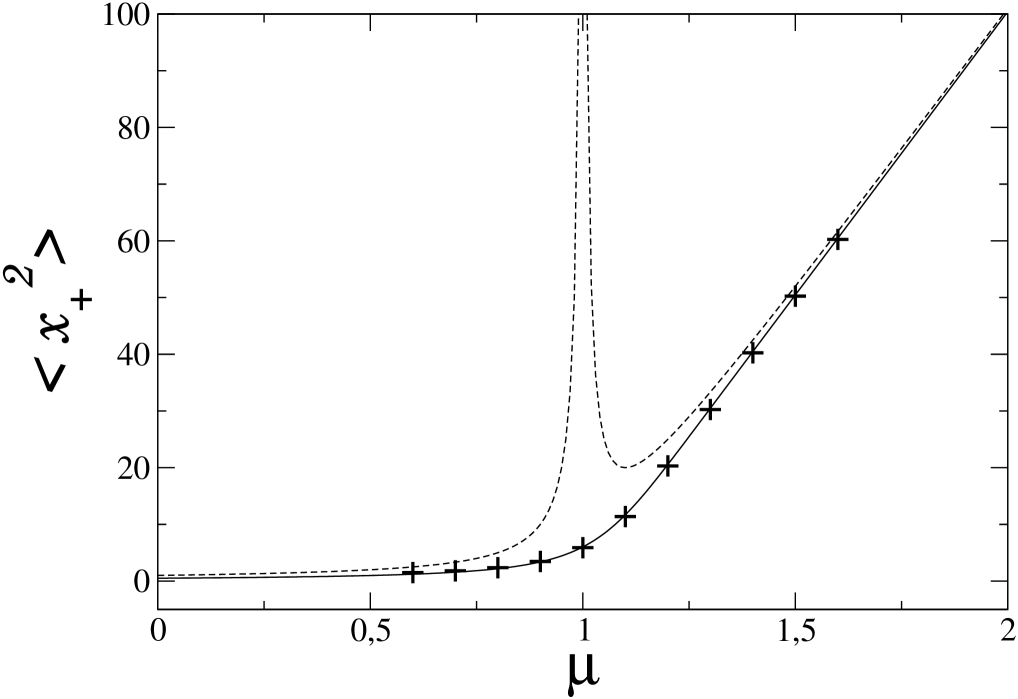
In Refs.mcneil ; singh Fokker-Planck equations were derived for the complex-P mcneil and positive-P singh representations, and stationary solutions were obtained for the corresponding distributions. Since these Fokker-Planck equations were derived without any truncation, we can consider the stationary distributions so obtained as exact. In Ref.karen an exact stationary Wigner function was mapped from the complex-P distribution of Ref.mcneil and expressed in terms of Bessel functions. It is important to remark that the simple Wigner function presented here provides a very good approximation for those exact solutions, as can be seen in Figs.3 and 4, even for a rather large value for the nonlinear coupling $g^{2}$.

Figure 4: Comparison between the values of the squeezed variable $\langle x^{2}_{-}\rangle$ obtained from the linearized theory (solid line) with those obtained from the Wigner function of Ref. karen (circles), and the one given by Eq.(14) (crosses). In all cases, we have set $g^{2}=0.01$.

IV Conclusion

By truncating the evolution equation for the two-mode Wigner function of an optical parametric oscillator, we derived a Fokker-Planck equation which admits a simple potential solution in any operation regime of the OPO. For the unsqueezed quadratures, this solution does not present the unphysical divergent behavior of the linearized theory on the oscillation threshold. Moreover, it provides good agreement with exact quasiprobabilities already available in the literature, both for the squeezed and unsqueezed quadratures. While these exact solutions are given as infinite series, the potential solution of the truncated Wigner distribution presents a simple form allowing for an easier visualization of the phase space distribution.