The chemical abundance analysis of normal early A- and late B-type stars

Abstract

Context. Modern spectroscopy of early-type stars often aims at studying complex physical phenomena such as stellar pulsation, the peculiarity of the composition of the photosphere, chemical stratification, the presence of a magnetic field, and its interplay with the stellar atmosphere and the circumstellar environment. Comparatively less attention is paid to identifying and studying the ”normal” A- and B-type stars and testing how the basic atomic parameters and standard spectral analysis allow one to fit the observations. By contrast, this kind of study is paramount eventually for allowing one to correctly quantify the impact of the various physical processes that occur inside the atmospheres of A- and B-type stars.

Aims. We wish to establish whether the chemical composition of the solar photosphere can be regarded as a reference for early A- and late B-type stars.

Methods. We have obtained optical high-resolution, high signal-to-noise ratio spectra of three slowly rotating early-type stars (HD 145788, 21 Peg and $\pi$ Cet) that show no obvious sign of chemical peculiarity, and performed a very accurate LTE abundance analysis of up to 38 ions of 26 elements (for 21 Peg), using a vast amount of spectral lines visible in the spectral region covered by our spectra.

Results. We provide an exhaustive description of the abundance characteristics of the three analysed stars with a critical review of the line parameters used to derive the abundances. We compiled a table of atomic data for more than 1100 measured lines that may be used in the future as a reference. The abundances we obtained for He, C, Al, S, V, Cr, Mn, Fe, Ni, Sr, Y, and Zr are compatible with the solar ones derived with recent 3D radiative-hydrodynamical simulations of the solar photosphere. The abundances of the remaining studied elements show some degree of discrepancy compared to the solar photosphere. Those of N, Na, Mg, Si, Ca, Ti, and Nd may well be ascribed to non-LTE effects; for P, Cl, Sc and Co, non-LTE effects are totally unknown; O, Ne, Ar, and Ba show discrepancies that cannot be ascribed to non-LTE effects. The discrepancies obtained for O (in two stars) and Ne agree with very recent non-LTE abundance analysis of early B-type stars in the solar neighbourhood.

1 Introduction

In the last decade there has been dramatic improvement in the tools for the analysis of optical stellar spectra, both from the observational and theoretical perspective. New high-resolution echelle instruments have come online, which cover much broader spectral ranges than older single-order spectrographs. Data quality has also substantially improved in terms of signal-to-noise ratio (SNR), because of substantially greater instrument efficiency, and the use of large-size telescopes. Thanks to the vibrant observational activities of the past few years, and thanks to efficient and user-friendly data archive facilities, a huge high-quality spectroscopic database is now available to the public.

With the development of powerful and cheap computers, it has become practical to exploit these new data by performing spectral analysis using large spectral windows rather than selected spectral lines, at a level of realism heretofore impossible. The high accuracy of observations and modelling techniques now allows, for example, stretching the realm of abundance analysis to faster rotators than was possible in the past, but also provides the possibility of learning more about the structure of the stellar atmospheres and the ongoing physical processes, especially when spectral synthesis fails to reproduce the observations. For instance, observed discrepancies between observed and synthetic spectra have allowed us to discover that the signature of chemical stratification is ubiquitous in the spectra of some chemically peculiar stars (Bagnulo et al. 2001; Wade et al. 2001; Ryabchikova et al. 2003) and to perform accurate modelling of this stratification in the atmospheres of Ap stars (for instance, Ryabchikova et al. 2005; Kochukhov et al. 2006).

However, our inability to reproduce observations frequently stems for a very simple cause: that atomic data for individual spectral lines are incorrect. For solar type stars it is possible to construct a ”reference” list of reliable spectral lines with reliable atomic data through the comparison of synthetic spectra with the solar observed spectrum, since the solar abundances are accurately known. In many cases, however, the solar spectrum cannot provide the required information, because the temperature of the target stars is significantly different from that of the sun. This problem can be overcome by adopting an analogous reference at a temperature reasonably close to the target temperature. The method involves a selection of a set of suitable reference stars for which very high quality spectra are available. Then an accurate determination of the stellar photospheric parameters and an accurate abundance analysis are performed with the largest possible number of spectral lines and the best possible atomic data. Finally, those spectral lines exhibiting the largest discrepancies from the model fit are identified, and their atomic data revised by assuming that the average abundance (inferred from the complete sample of spectral lines of that element) is the correct one. In this process it is important to take effects into account that can potentially play a significant role in all stellar atmospheres, such as variations in the model structure from non-solar abundances and non-LTE effects.

In this paper we address the problem of establishing references for effective temperatures around 10000–13000 K. This is in some respect the easiest temperature range to study, as well as one of the most interesting. This temperature is close to ideal because the spectra of stars in this interval are generally unaffected by severe blending. It is also relevant because stars in this temperature range display spectroscopic peculiarities (chemical abundance peculiarities, stratification, Zeeman effect, etc.) that reflect physical conditions and processes of interest for detailed investigation. A crucial prerequisite for studying and characterising these phenomena is the capacity to model the underlying stellar spectrum in detail, and this requires high quality atomic data.

The highest degree of accuracy in abundance analysis is reached for sharp-lined stars. Unfortunately, these objects are quite rare among A- and B-type stars, which are generally characterised by high rotational velocities. Furthermore, most of the slowly rotating stars in the chosen temperature region belong to various groups of magnetic and non-magnetic, chemically peculiar objects. As a matter of fact, many previous studies aimed at determining the chemical composition of ”normal” early A- and late B-type stars were based on samples ”polluted” by moderately chemically peculiar stars. For instance, the work by Hempel & Holweger (2003) includes the sharp-lined HgMn star 53 Aur. Hill & Landstreet (1993) searched for compositional differences among A-type stars, but four out of six programme stars are in fact classified as hot Am stars on the basis of the abundances of the heavy elements Sr-Y-Zr-Ba, which are considered as diffusion indicators (i.e., Sirius, $o$ Peg, and $\theta$ Leo, see Hempel & Holweger 2003). The complexity of the problem of distinguishing between normal A and marginal Am stars is further stressed by Adelman & Unsuree (2007). The aim of the present paper is to search for sharp-lined early A- or late B-type stars with a chemical composition as close as possible to the solar one. As a final outcome, one could assess whether the chemical composition of the solar photosphere may be considered at least in principle as a reference for the composition of the early A- and late B-type stars. If such a star is found, this will not imply that the solar composition is the most characteristic for the slowly rotating A- and B-type stars, but will be used as further evidence that any departure from the composition of the solar photosphere has to be explained in terms of diffusion or other physical mechanisms that are not active at the same efficiency level in the solar photosphere.

Our work is based on a very detailed and accurate study of a vast sample of spectral lines. As a by-product, we provide a list of more than 1100 spectral lines from which we have assessed the accuracy of the corresponding atomic data. Such a list may serve as a future reference for further abundance analysis studies of stars with a similar spectral type.

This paper is organised as follows. Sect. 2 describes the target selection, observations and data reduction, Sect. 3 presents methods and results for the choice of the best fundamental parameters that describe the atmospheres of the programme stars, Sect. 4 presents the methods and results of the abundance analysis of the programme stars. Our results are finally discussed in Sect. 5.

2 Target selection, observations, and data reduction

For our analysis we need a late A-type or early B-type star with a sharp-line spectrum (hence the star must have a small ${\upsilon}\sin i$) and one exhibiting the least possible complications due to phenomena such as non-homogeneous surface distribution of chemical elements, pulsation, or a magnetic field. Finding such a target is not a simple task, because most of the early-type stars are fast rotators. Slowly rotating A- and B-type stars generally show some type of chemical peculiarity often associated to the presence of abundance patches, a magnetic field (which broadens, or even splits spectral lines), and chemical stratification. Even Vega, which has been considered for a long time as the prototype of a ”normal”, slow rotating A-type star, is in fact currently classified as a $\lambda$ Boo star and discovered to actually be a fast rotating star seen pole-on, exhibiting, as such, distorted line profiles (Adelman & Gulliver 1990; Yoon et al. 2008). Based on our knowledge, we reached the conclusion that the most suitable target for our project is the B9 star 21 Peg (HD 209459), which is known from previous studies as a ”normal” single star with ${\upsilon}\sin i\sim 4$ $\mathrm{km\,s}^{-1}$ (see, e.g. Sadakane 1981).

We felt it was necessary to consider additional targets of our spectral analysis, for two main reasons. Since we intend to provide an accurate reference for the typical abundances of the chemical elements in A- and B-type stars (and compare these values with the solar ones), we need to cross-check with further examples whether the results obtained for 21 Peg are similar to those of other ”normal”, slow rotating A-type stars. Second, to check the accuracy of the astrophysical measurements of the log$gf$ values, which is a natural complement of the present work. Both these goals are best achieved with the use of abundance values that have been obtained with a homogeneous method, rather than from a mixed collection of data from the literature. Therefore, we have also analysed another two stars of similar temperature as 21 Peg, i.e., HD 145788 (HR 6041) and $\pi$ Cet (HR 811). Both stars fulfill our requirements, although are slightly less ideal than 21 Peg. HD 145788, suggested to us by Prof. Fekel, is a slowly rotating single star with ${\upsilon}\sin i$ $\sim$ 8 $\mathrm{km\,s}^{-1}$(Fekel 2003). $\pi$ Cet, a SB1 with ${\upsilon}\sin i\sim 20$ $\mathrm{km\,s}^{-1}$, shows an infrared excess, and is a suspected Herbig Ae/Be star (Malfait et al. 1998). Since its spectrum is not visibly contaminated by the companion, it still serves our purpose. $\pi$ Cet was also already used as a normal comparison star in the abundance study of chemically peculiar stars by Smith & Dworetsky (1993).

The star 21 Peg was observed five times during two observing nights in August 2007, with the FIES instrument of the North Optical Telescope (NOT). FIES is a cross-dispersed high-resolution échelle spectrograph that offers a maximum spectral resolution of R = 65 000, covering the entire spectral range 3700–7400 Å.

Data were reduced using a pipeline developed by D. Lyashko, which is based on the one described by Tsymbal et al. (2003). All bias and flat-field images were median-averaged before calibration, and the scattered light was subtracted by using a 2D background approximation. For cleaning cosmic ray hits, an algorithm that compares the direct and reversed observed spectral profiles was adopted. To determine the boundaries of echelle orders, the code uses a special template for each order position in each row across the dispersion axis. The shift of the row spectra relative to the template was derived by a cross-correlation technique. Wavelength calibration of each image was based on a single ThAr exposure, recorded immediately after the respective stellar time series, and calibrated by a 2D approximation of the dispersion surface. An internal accuracy of $\sim 100$ ms^-1 was achieved by using several hundred ThAr lines in every echelle order.

Each reduced spectrum has a SNR per pixel of about 300 at 5000 Å. All five spectra are fully consistent among themselves, which confirms that the star is not variable. This allowed us to combine all data in a unique spectrum with a final SNR of about 700.

Because of the very low ${\upsilon}\sin i$ of 21 Peg, we made use of a very high-resolution spectrum ($R=120\,000$) obtained with the Gecko instrument (now decommissioned) of the Canada-France-Hawaii Telescope (CFHT, Landstreet 1998) to measure this parameter. The spectrum covers the ranges 4612–4640 Å and 5160–5192 Å, which are too short to perform a full spectral analysis, but sufficient to measure ${\upsilon}\sin i$ with high accuracy. According to Hubrig et al. (2006) the mean longitudinal magnetic field of 21 Peg is $-$144$\pm$60 G, which excludes the possibility that the star has a structured magnetic field.

The spectrum of HD 145788 was obtained with the cross-dispersed échelle spectrograph HARPS instrument attached at the 3.6-m ESO La Silla telescope, with an exposure time of 120 s, and reduced with the online pipeline . The reduced spectrum has a resolution of 115 000, and a SNR per pixel of about 200 at 5000 Å. The spectral range is 3780–6910 Å with a gap between 5300 Å and 5330 Å, because one echelle order is lost in the gap between the two chips of the CCD mosaic detector.

The star $\pi$ Cet was observed with the ESPaDOnS instrument of the CHFT February, 20 and 21 2005. ESPaDOnS consists of a table-top, cross-dispersed echelle spectrograph fed via a double optical fiber directly from a Cassegrain-mounted polarisation analysis module. Both Stokes $I$ and $V$ spectra were obtained throughout the spectral range 3700 to 10400 Å at a resolution of about 65 000. The spectra were reduced using the Libre-ESpRIT reduction package Donati et al. (1997, and in prep.). The two spectra (each obtained from the combination of four 120 s sub-exposures) were combined into a final spectrum that has an SNR per pixel of about 1200 at 5000 Å.

The observation of $\pi$ Cet enters in the context of a large spectropolarimetric survey of Herbig Ae/Be stars. Least-squares deconvolution (LSD, Donati et al. 1997) was applied to the spectra of $\pi$ Cet assuming a solar abundance line mask corresponding to an effective temperature of 13000 K. The resulting LSD profiles show a clean, relatively sharp mean Stokes $I$ profile, corresponding to ${\upsilon}\sin i=20\pm 1$ $\mathrm{km\,s}^{-1}$, and no detection of any Stokes $V$ signature indicative of a photospheric magnetic field. Integration of Stokes $V$ across the line using Eq. (1) of Wade et al. (2000) yields longitudinal magnetic fields consistent with zero field and with formal 1$\sigma$ uncertainties of about 10 G. The high-resolution spectropolarimetric measurements therefore provide no evidence of magnetic fields in the photospheric layers of the star.

All the spectra of the three stars were normalised by fitting a spline to carefully selected continuum points. For each object, radial velocities ${\upsilon}_{\mathrm{r}}$ were determined by computing the median of the results obtained by fitting synthetic line profiles of several individual carefully selected lines into the observed spectrum. The ${\upsilon}_{\mathrm{r}}$ values are listed in Table 1, and their uncertainty is of the order of 0.5 $\mathrm{km\,s}^{-1}$. The spectra were then shifted to the wavelength rest frame. Selected spectral windows containing the observed blue He i lines, together with the synthetic profiles, are displayed in Fig. 1.

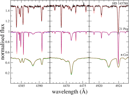
Figure 1: Samples of the spectra of HD 145788, 21 Peg and $\pi$ Cet around three He i lines: 4387 Å, 4471 Å and 4921 Å in comparison with our final synthetic profiles (dashed lines) calculated for each line. The spectra of HD 145788 and $\pi$ Cet are shifted upwards and downwards of 0.5, respectively.

3 Fundamental parameters

Fundamental parameters for the atmospheric models were obtained using photometric indicators as a first guess. For their refined estimate, we performed a spectroscopic analysis of hydrogen lines and metal lines, and as a final step, compared the observed and computed energy distributions. The spectroscopic tuning of the fundamental parameters is needed since different photometries and calibrations would give different parameters and uncertainties. The spectroscopic analysis will provide a set of parameters that fit all the parameter indicators consistently, with less uncertainties. Model atmospheres were calculated with LLmodels, an LTE code that uses direct sampling of the line opacities (Shulyak et al. 2004) and allows computing models with an individualised abundance pattern. Atomic parameters of spectral lines used for model atmosphere calculations were extracted from the VALD database (Piskunov et al. 1995; Kupka et al. 1999; Ryabchikova et al. 1999).

Before applying the spectroscopic method, we estimated the star’s ${\upsilon}\sin i$. For 21 Peg, a ${\upsilon}\sin i$ value of $3.76\pm 0.35$ $\mathrm{km\,s}^{-1}$ was derived from the fit with a synthetic spectrum to 21 carefully selected lines observed with the Gecko instrument. This value agrees very well with the 3.9 $\mathrm{km\,s}^{-1}$ value derived by Landstreet (1998). Achieving such high precision was possible thanks to the high quality of the spectrum and the low ${\upsilon}\sin i$. The ${\upsilon}\sin i$ values for HD 145788 and $\pi$ Cet, $10.0\pm 0.5$ $\mathrm{km\,s}^{-1}$ and $20.2\pm 0.9$ $\mathrm{km\,s}^{-1}$, respectively, were derived from fitting about 20 well-selected lines along the whole available spectral region.

In the next sections, we describe the determination of the atmospheric parameters: $T_{\mathrm{eff}}$, effective gravity ($\log g$), and microturbulent velocity ($\upsilon_{\mathrm{mic}}$), and their uncertainties. The fundamental parameters finally adopted for 21 Peg, HD 145788, and $\pi$ Cet are given in Table 1.

Table 1: Adopted atmospheric parameters for the analysed stars.

Star	$T_{\mathrm{eff}}$	$\log g$	$\upsilon_{\mathrm{mic}}$	$\sigma_{\upsilon_{\mathrm{mic}}}$	${\upsilon}\sin i$	$\sigma_{{\upsilon}\sin i}$	${\upsilon}_{\mathrm{r}}$
Name	[K]	[cgs]	[$\mathrm{km\,s}^{-1}$]	[$\mathrm{km\,s}^{-1}$]	[$\mathrm{km\,s}^{-1}$]	[$\mathrm{km\,s}^{-1}$]	[$\mathrm{km\,s}^{-1}$]
21 Peg	10400	3.55	0.5	0.4	3.76	0.35	0.5
HD 145788	9750	3.70	1.3	0.2	10.0	0.5	$-$13.9
$\pi$ Cet	12800	3.75	1.0	0.5	20.2	0.9	12.5

The uncertainties on $T_{\mathrm{eff}}$, $\log g$, and ${\upsilon}_{\mathrm{r}}$ are 200 K, 0.1 dex, and 0.5 $\mathrm{km\,s}^{-1}$, respectively.

3.1 Photometric indicators

Since none of the three programme stars, HD 145788, 21 Peg or $\pi$ Cet are known to be photometrically variable or peculiar, we can use temperature and gravity calibrations of different photometric indices for normal stars to get a preliminary estimate of the atmospheric parameters. The effective temperature ($T_{\mathrm{eff}}$) and gravity ($\log g$) were derived from Strömgren photometry (Hauck & Mermilliod 1998) with calibrations by Moon & Dworetsky (1985) and by Napiwotzki et al. (1993), and from Geneva photometry (Rufener 1988) with the calibration by North & Nicolet (1990). The mean parameters from the three calibrations that were used as starting models are the following ones: $T_{\mathrm{eff}}$ = 9675$\pm$75 K, $\log g$ = 3.72$\pm$0.03 for HD 145788; $T_{\mathrm{eff}}$ = 10255$\pm$115 K, $\log g$ = 3.51 for 21 Peg; $T_{\mathrm{eff}}$ = 13200$\pm$65 K $\log g$ = 3.77$\pm$0.15 for $\pi$ Cet. No error bar is given for the $\log g$ of 21 Peg since all three calibrations give the same value.

3.2 Spectroscopic indicators

3.2.1 Hydrogen lines

For a fully consistent abundance analysis, the photometric parameters have to be checked and eventually tuned according to spectroscopic indicators, such as hydrogen line profiles. In the temperature range where HD 145788, 21 Peg, and $\pi$ Cet lie, the hydrogen line wings are less sensitive to $T_{\mathrm{eff}}$ than to $\log g$ variations, but temperature effects can still be visible in the part of the wings close to the line core. For this reason hydrogen lines are very important not only for our analysis, but in general for every consistent parameter determination. To spectroscopically derive the fundamental parameters from hydrogen lines, we fitted synthetic line profiles, calculated with Synth3 (Kochukhov 2007), to the observed profiles. Synth3 incorporates the code by Barklem et al. (2000) that takes into account not only self-broadening but also Stark broadening (see their Sect. 3). For the latter, the default mode of Synth3, adopted in this work, uses an improved and extended HLINOP routine (Kurucz 1993).

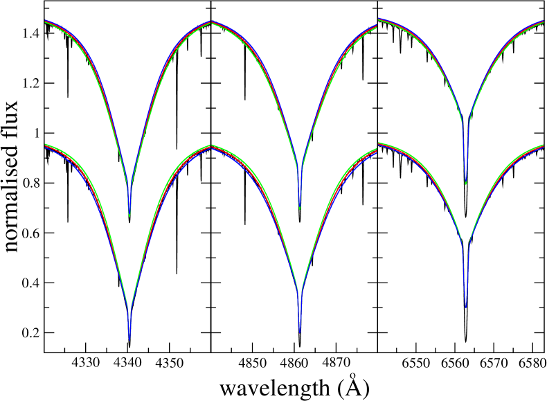
Figure 8: Same as Fig. 2, but also for H$\gamma$ and H$\alpha$.

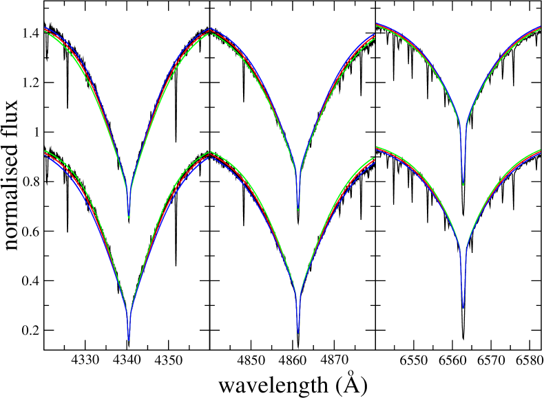
Figure 9: Same as Fig. 8, but for HD 145788.

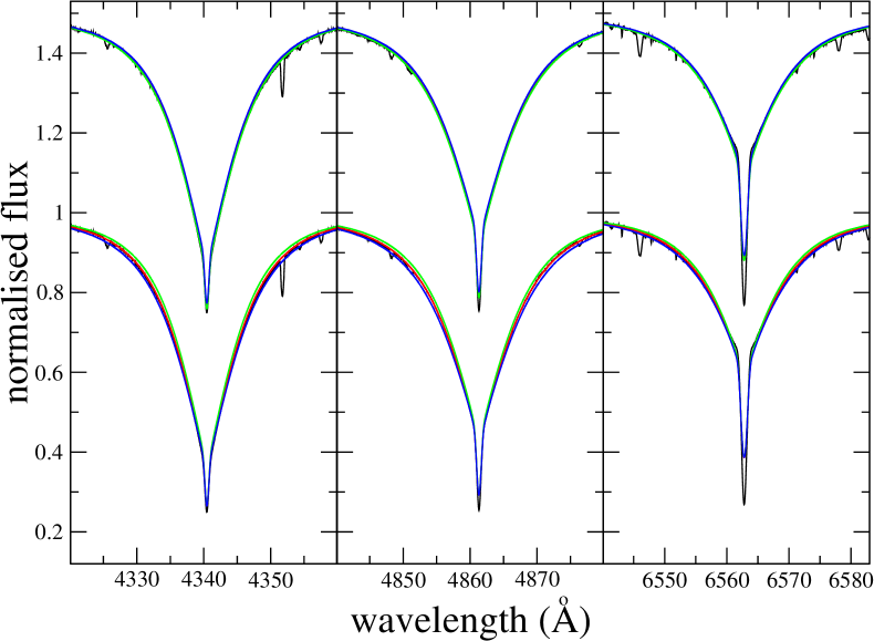
Figure 10: Same as Fig. 8, but for $\pi$ Cet.

Figure 2 shows the comparison between the observed H$\beta$ line profile for 21 Peg and the synthetic profiles calculated with the adopted stellar parameters. In Fig. 2 we also added the synthetic line profiles calculated with 1$\sigma$ error bars on $T_{\mathrm{eff}}$  ($\pm$ 200 K; upper profile) and $\log g$  ($\pm$ 0.1 dex; lower profile). The same profiles with the same uncertainties, but for H$\gamma$, H$\beta$, and H$\alpha$ (from left to right) for the three programme stars, are shown in Figs. 9, 8, and 10 (online material).

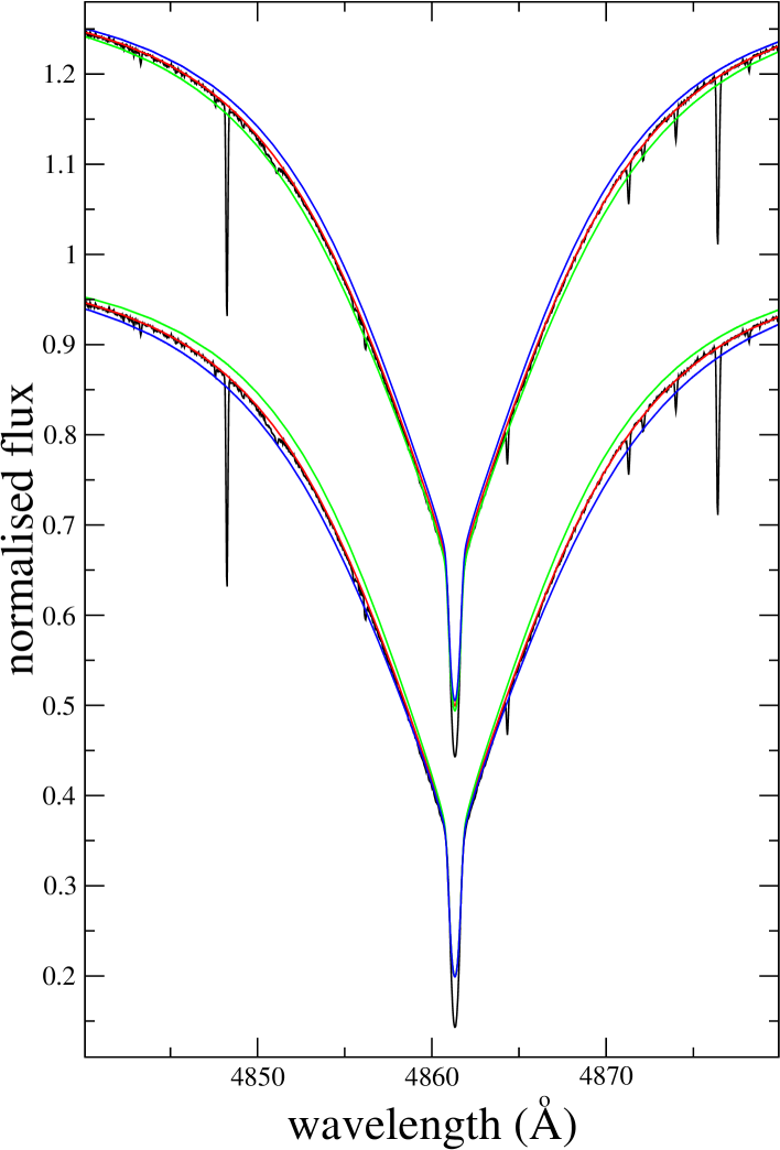
Figure 2: Observed H$\beta$ line profile for 21 Peg (black solid line), compared to synthetic profiles (red, blue, and green lines). The red solid lines were obtained assuming the best $T_{\mathrm{eff}}$ and $\log g$ values of Table 1. The blue lines show the synthetic profile by increasing $T_{\mathrm{eff}}$ by 200 K (top spectrum) or $\log g$ by 0.1 dex (bottom spectrum). The green lines show the synthetic profile by decreasing $T_{\mathrm{eff}}$ by 200 K (top spectrum) or $\log g$ by 0.1 dex (bottom spectrum).

The three hydrogen lines (H$\gamma$, H$\beta$, and H$\alpha$) used to spectroscopically improve the fundamental parameters for HD 145788 gave slightly different results both for $T_{\mathrm{eff}}$ and for $\log g$. As final values, we took their mean ($T_{\mathrm{eff}}$ = 9750 K; $\log g$ = 3.7). This discrepancy is visible in Fig. 9 (online material), but it lies within the errors given for $T_{\mathrm{eff}}$ and $\log g$. The spectrum of HD 145788 also allowed a good normalisation of the region bluer than H$\gamma$. We synthesised this region to check the quality of our final fundamental parameters finding a very good fit for the three hydrogen lines H$\delta$, H$\epsilon$, and H₈.

For 21 Peg we obtained the same temperature estimates from H$\alpha$ and H$\beta$ ($T_{\mathrm{eff}}$ = 10400 K) and by 200 K less from the fitting of H$\gamma$. We adopted a final $T_{\mathrm{eff}}$ of 10400 K. To fit all three hydrogen lines, we need slightly different values of $\log g$: 3.47 for H$\gamma$, 3.54 for H$\beta$ and 3.57 for H$\alpha$. We finally adopted $\log g$ = 3.55 taking possible continuum normalisation problems into account, in particular, for H$\gamma$.

The temperature determination for $\pi$ Cet was more difficult thanks to the weak effect that this parameter has on the hydrogen lines at about 13000 K and to the slightly peculiar shape of the H$\alpha$ line. As explained in Sect. 5, $\pi$ Cet probably shows a small emission signature in the region around the core of H$\alpha$ possibly because of a circumstellar disk. This region is the one where $T_{\mathrm{eff}}$ effects are visible, making it almost impossible to obtain a good temperature determination from this line. H$\gamma$ and H$\beta$ gave best temperatures of 12700 K and 12900 K, respectively, leading to a final adopted value of 12800 K. Confirmation of this value was then given by the spectrophotometry (see Sect. 3.3). The results of LTE abundance analysis (Sect. 4) show that $\pi$ Cet has little He overabundance that leads to an overestimation of $\log g$ if the He abundance is not taken into account in the model atmosphere calculation (Auer et al. 1966). For this reason we derived the first set of fundamental parameters ($T_{\mathrm{eff}}$ = 12800 K; $\log g$ = 3.80) and then the He abundance ($\log(N_{\rm He}/N_{\rm tot})$ = $-$0.97 dex). As a next step we recalculated a set of model atmospheres with the derived He abundance and re-fit the hydrogen line profiles. The best-fit gave us the same temperature, but weak effective gravity ($\log g$ = 3.75). As expected, the He overabundance is acting as pressure, requiring an adjustment of $\log g$ to be balanced. We obtained the He abundance from the fitting of the blue He line wings. The blue He lines are, in general, considered as showing very little non-LTE effect (Leone & Lanzafame 1998), and as we only used the line wings, this leads us to conclude that our results should not be affected by non-LTE effects and that the He is overabundant in $\pi$ Cet. The best fit to the blue He i lines of $\pi$ Cet is shown in Fig. 1.

The example of $\pi$ Cet is important because it clearly shows the effect of the single element abundance on the parameter determination, not only for chemically peculiar stars (for which this effect is well known and often, but not always, taken into account), but also for chemically ”normal” stars.

The set of parameters that best fit the hydrogen line profiles could not be unique. For 21 Peg, we checked that using a combination of a lower temperature and lower gravity or else higher temperature and higher gravity increases the standard deviation of the fit of the H$\beta$ line wings by $\sim$25%. The result is that a different combination of $T_{\mathrm{eff}}$ and $\log g$ could in principle provide a similar fit. For this reason the derived fundamental parameters should be checked with other indicators, such as the analysis of metallic lines (ionisation and excitation equilibrium) and the fitting of the spectral energy distribution. The latter is more important because ionisation and excitation equilibrium should be strictly used only with a full non-LTE treatment of the line formation.

3.2.2 Metallic lines

The metallic-line spectrum may also provide constraints on the atmospheric parameters. If no deviation from the local thermodynamic equilibrium (LTE) is expected, the minimisation of the correlation between individual line abundances and excitation potential, for a certain element/ion, allows one to check the determined $T_{\mathrm{eff}}$. Then the balance between different ionisation stages of the same element provides a check for $\log g$. The microturbulent velocity, $\upsilon_{\mathrm{mic}}$ is then determined by minimising the correlation between individual abundances and equivalent widths for a certain element. Determining the fundamental parameters performed in this way has to be done iteratively since, for example, a variation in $T_{\mathrm{eff}}$ leads to a change in the best $\log g$ and $\upsilon_{\mathrm{mic}}$.

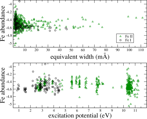
Figure 3: Iron abundance vs. equivalent widths (upper panel) and excitation potential (lower panel) for 21 Peg. The open circles indicate Fe i, while the open triangles indicate Fe ii.

Figure 3 shows the correlations of Fe i and Fe ii abundances with the equivalent widths (upper panel) and with the excitation potential (lower panel) for 21 Peg. The correlation with the equivalent widths is shown for a $\upsilon_{\mathrm{mic}}$ of 0.5 $\mathrm{km\,s}^{-1}$, which we infer to be the best value for 21 Peg, since the slope of the linear fit for Fe i is $-4.897\times 10^{-3}\pm 1.560\times 10^{-3}$ mÅ^-1 and for Fe ii is $2.146\times 10^{-5}\pm 4.058\times 10^{-4}$ mÅ^-1. Here we gave a preference to the result obtained from Fe ii because of the higher number of measured Fe ii lines in a wider range of equivalent widths. The same analysis was made for HD 145788 and for $\pi$ Cet. The error bar on $\upsilon_{\mathrm{mic}}$ was calculated using the error bar of the slope (abundance vs. equivalent width) derived from a set of different $\upsilon_{\mathrm{mic}}$. The uncertainties listed in Table 1 are given considering 2$\sigma$ on the error bar of the derived slopes. Considering a 1$\sigma$ error bar, the uncertainties on $\upsilon_{\mathrm{mic}}$ are of 0.1 $\mathrm{km\,s}^{-1}$for HD 145788 and 21 Peg and of 0.2 $\mathrm{km\,s}^{-1}$ for $\pi$ Cet.

According to previous works, deviation from LTE of the Fe ii lines is expected to be very small ($\sim$ 0.02 dex Gigas 1986; Rentzsch-Holm 1996) for the analysed stars, such that the absence of any clear correlation between the line Fe ii abundance and the excitation potential confirms the $T_{\mathrm{eff}}$ derived from the hydrogen lines.

For the Fe i lines, deviations from LTE of about $+$0.3 dex are given by Gigas (1986) and Rentzsch-Holm (1996). However, both Gigas (1986) and Rentzsch-Holm (1996), as well as Hempel & Holweger (2003), used the same model atom, which includes 79 Fe i and 20 Fe ii energy levels. We note that the highest energy level in their model atom for Fe ii has an excitation energy of about 6 eV, while the ionisation potential is 16.17 eV. Such a model atom does not provide collisional coupling of Fe ii to Fe iii, which operates for the majority of iron atoms in line formation layers below $\log\tau_{5000}=-1$. Unfortunately, the existing NLTE calculations for Fe are not accurate enough to be applied now to our stars. Clearly, an extended energy-level model atom is needed for a reliable non-LTE analysis of Fe. The ionisation equilibrium for different elements/ions (or its violation) can be seen in Table 4 and is discussed in Sect. 4.

3.3 Spectrophotometry

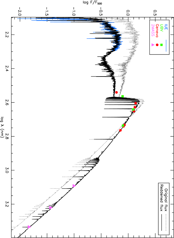
Figure 11: Comparison between LLmodels theoretical fluxes calculated with the fundamental parameters and abundances derived for HD 145788, taking into account a reddening of E(B-V)=0.20 (full black line) and without taking into account reddening (dashed black line), with IUE calibrated fluxes (full blue line), Johnson UBV photometry (green squares), Geneva photometry (red circles) and 2MASS photmetry (violet triangles). The model fluxes were convolved to have approximately the same spectral resolution of the IUE fluxes (R $\sim$ 900).

For a complete self-consistent analysis of any star, one should reproduce the observed spectral energy distribution with the adopted parameters for a model atmosphere. In the optical spectral region, spectrophotometry was only available for 21 Peg and $\pi$ Cet, while in the ultraviolet, IUE spectra were available for all three stars. For $\pi$ Cet ultraviolet spectrophotometry from the TD-1 satellite (Jamar et al. 1976) was also available, along with the flux calibrated spectra from STIS at HST (Gregg et al. 2004). The comparison between the observed flux distributions and the model fluxes calculated with the adopted atmospheric parameters for 21 Peg and $\pi$ Cet is shown in Fig. 4. For HD 145788 we estimated a reddening E(B-V)$\approx$0.2 from the dust maps of Schlegel et al. (1998). The comparison of reddened model fluxes with the available IUE spectrum, Johnson UBV photometry (Nicolet 1978), Geneva photometry and 2MASS photometry (Cutri et al. 2003) is shown in Fig. 11 (online material). This plots supports the value of E(B-V)=0.2 and shows good agreement between all the observations and the model fluxes, confirming the obtained fundamental parameters, and also the importance of considering reddening in the analysis of relatively nearby stars such as HD 145788.

The optical spectrophotometry was taken from Adelman et al. (1989) and Breger (1976). All flux measurements were normalised to the flux value at 5000 Å obtained from observed data for $\pi$ Cet and 21 Peg and from the model fluxes for HD 145788. Also for 21 Peg and $\pi$ Cet, we extended the comparison to the near infrared region including 2MASS photometry (Cutri et al. 2003). Following Netopil et al. (2008), we obtained a reddening E(B-V)$\leq 0.01\pm 0.01$ mag for both $\pi$ Cet and 21 Peg. A good agreement between the unreddened model fluxes and the observed spectrophotometry from UV to near infrared confirms negligible reddening for these two stars.

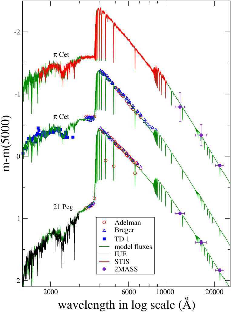
Figure 4: Comparison between LLmodels theoretical fluxes calculated with the fundamental parameters and abundances derived for 21 Peg and $\pi$ Cet (green solid line) with spectrophotometries by Adelman et al. (1989) (open red circles) and Breger (1976) (open blue triangles), IUE calibrated fluxes (full black line), TD 1 observations (full blue squares) and STIS spectrum (full red line). The violet full dots represent the 2MASS photometry for which the given error bar in wavelength shows the wavelength range covered by each filter. The model fluxes for 21 Peg and $\pi$ Cet, shown in the middle of the panel, were convolved to have the same spectral resolution of the IUE fluxes (R $\sim$ 900), while the upper of $\pi$ Cet has a spectral resolution 700, approximately the same of STIS spectra. For a better visualisation of the whole spectral region the x-axis is on a logarithmic scale.

The agreement between the IUE observation and the model fluxes is very good for HD 145788, but the IUE data alone cannot be used as a check of $T_{\mathrm{eff}}$, since a variation of about 1000–1500 K is needed to make any visible discrepancy. At the $T_{\mathrm{eff}}$ of HD 145788 hydrogen lines were still quite sensitive to temperature variations, so we did not need accurate spectrophotometry for a reliable effective temperature estimate. The slight disagreement between the model fluxes and the 2MASS photometry could stem from our not accounting for reddening in the calculation of the model fluxes since the derived value is too uncertain.

The model fluxes of 21 Peg are in good agreement with the observations from the ultraviolet up to the near infrared. For 21 Peg and $\pi$ Cet, few data points in the red appear above the model fluxes. This often happens with the optical spectrophotometry as shown in Fig. 1 of Adelman et al. (2002). We do not have a definite explanation for this effect, although taking a very accurate measurement of the reddening into account could remove this inconsistency. As for the hydrogen lines, we checked the fit of the spectral energy distribution to model fluxes calculated with a combination of a lower temperature and lower gravity or a higher temperature and higher gravity. In both cases the fit clearly becomes worse mainly in the spectral region around the Balmer jump. This definitively excludes the possibility that a combination of fundamental parameters, which gives a worse but still reasonable fit to the hydrogen line profiles, should considered.

For $\pi$ Cet we obtained several spectrophotometric observations from different sources. In particular, the data in the optical region around the Balmer jump were conclusive for $T_{\mathrm{eff}}$ determination, as mentioned already in Sect. 3.2.1. The STIS spectrum shown in Fig. 4 is formed by three separated spectra (UV, visible, IR) with about the same spectral resolution. We noticed a small (but not negligible) vertical jump at the overlapping wavelengths between the three spectra. For this reason we decided to fit them separately. This decision was based on an adjustment performed at the level of the flux calibration (Maíz-Apellániz 2005, 2006).

The use of an energy distribution plays a crucial role in adjusting the atmospheric parameters because it is independent of the photometric calibrations (different for each author), of the hydrogen line fitting (reduction and normalisation dependent), and of the ionisation equilibria approach (dependent on several effects such as the adopted atomic line data and non-LTE effects).

The uncertainties on $T_{\mathrm{eff}}$ and $\log g$ were derived from the hydrogen line fitting. This way of deriving the error bars on the parameters also includes the SNR of the observations. For all three stars, we derived an error bar on the $T_{\mathrm{eff}}$ of 200 K and 0.1 dex in $\log g$, as also shown in Figs. 8, 9, and 10 (online material).

3.4 Comparison with previous determinations

Only one previous temperature determination for HD 145788 is known. Glagolevskij (1994) determined a $T_{\mathrm{eff}}$ of 9600 K from the reddening free $Q$ parameter (Johnson & Morgan 1953) and of 9100 K from the $X$ parameter derived from multicolour photometry. The $T_{\mathrm{eff}}$ derived from the $Q$ parameter agrees with our estimation.

The star 21 Peg was analysed for abundances and atmospheric parameters several times in the past. The atmospheric parameters extracted from literature are collected in Table 2, together with the methods of their determination. The last column of Table 2 lists the methods adopted to derive the fundamental parameters for each author. SPh and JPh correspond to Strömgren and Johnson photometry respectively. ”Fe eq” indicates the use of the Fe ionisation equilibrium, while H-fit the use of hydrogen line fitting. SED corresponds to the use of spectral energy distribution in the visible and/or UV region. All the values obtained from the literature are in excellent agreement with our adopted parameters. We would like to mention that only the oldest determination (Sadakane 1981) was obtained using all the possible parameter indicators, as done in this work.

Table 2: Atmospheric parameters of 21 Peg derived from other authors.

Reference	$T_{\mathrm{eff}}$	$\log g$	method
	[K]	[cgs]
S81	10500	3.50	SPh, JPh, Fe eq, H-fit, SED
B82	10500	3.50	SPh, H-fit
A83	10700	(…)	JPh
A83	10350	(…)	SPh
A83	10375	(…)	SED
M85	10300	(…)	SED
S93	10450	3.50	SPh, H-fit
L98	10200	3.50	SPh
W00	10350	3.48	SPh
H01	10450	3.60	SPh
A02	10375	3.47	SPh
A02	10350	3.55	SED, H-fit
F09	10400	3.55	SED, H-fit

S81: Sadakane (1981), B82: Boesgaard et al. (1982), A83: Adelman & Pyper (1983), M85: Morossi & Malagnini (1985), S93: Smith & Dworetsky (1993), L98: Landstreet (1998), W00: Wahlgren & Hubrig (2000), H01: Hubrig & Castelli (2001), A02: Adelman et al. (2002) F09: this work.

The spectroscopic literature for $\pi$ Cet is extremely vast and started in the early 60s. We decided to compare the determinations of $T_{\mathrm{eff}}$ and $\log g$ from the late 70s on. These data and our determination are presented in Table 3. Our value for $T_{\mathrm{eff}}$ is the only one below 13000 K, while $\log g$ agrees with all the other measurements. Adelman et al. (2002) also derived the parameters of $\pi$ Cet with the simultaneous fitting of H$\gamma$ and spectrophotometry, essentially the same way as we did. The main difference is that they only used one available spectrophotometric set, while we used all the data found in the literature. The spectrophotometry by Breger (1976) appears a little below the one by Adelman et al. (1989) around the Balmer jump. To be able to simultaneously fit both sets of measurements, we needed a $T_{\mathrm{eff}}$ lower than 13000 K and the best fit was obtained for $T_{\mathrm{eff}}$ = 12800 K. Also our H$\beta$ profile is best-fitted only with a $T_{\mathrm{eff}}$ below 13000 K, as already mentioned in Sect. 3.2.1.

Table 3: Atmospheric parameters of $\pi$ Cet derived from other authors.

Reference	$T_{\mathrm{eff}}$	$\log g$	method
	[K]	[cgs]	(as in Table 2)
H79	13100	3.90	SPh
K80	13000	(…)	SED
M83	13030	3.88	SED(UV)
M83	13170	3.91	SED(visible)
A84	13150	3.65	SED, H-fit
M85	13170	(…)	SED
S88	13200	3.70	SED
M88	13425	(…)	SPh
R90	13150	3.50	SPh
A91	13150	3.85	H-fit
T91	13000	(…)	SED
S92	13210	3.65	SPh
A02	13174	3.70	SPh
A02	13100	3.85	SED, H-fit
F09	12800	3.75	SED, H-fit

H79: Heacox (1979), K80: Kontizas & Theodossiou (1980), M83: Malagnini et al. (1983), A84: Adelman (1984), M85: Morossi & Malagnini (1985), S88: Sadakane et al. (1988) M88: Megessier (1988), R90: Roby & Lambert (1990), A91: Adelman (1991) T91: Theodossiou & Danezis (1991), S92: Singh & Castelli (1992), A02: Adelman et al. (2002) F09: this work. The methods and the acronyms are as in Table 2.

4 Abundance analysis

The VALD database is the main source for the atomic parameters of spectral lines. For light elements C, N, O, Ne i, Mg i, Si ii, Si iii, S, Ar, and also for Fe iii, the oscillator strengths are taken from NIST online database (Ralchenko et al. 2008). LTE abundance analysis in the atmospheres of all three stars is based mainly on the equivalent widths analysed with the improved version of WIDTH9 code updated to use the VALD output linelists and kindly provided to us by V. Tsymbal.

In the case of blended lines or when the line is situated in the wings of the hydrogen lines, we performed synthetic spectrum calculations with the Synth3 code. For our analysis we used the maximum number of spectral lines available in the observed wavelength ranges except lines in spectral regions where the continuum normalisation was too uncertain (high orders of the Paschen series in the ESPaDOnS spectrum of $\pi$ Cet, for example). The final abundances are given in Table 4. A line-by-line abundance list with the equivalent width measurements, adopted oscillator strengths, and their sources is given in Table LABEL:line_abund (online material). Below we discuss the results obtained for individual elements.

Table 4: LTE atmospheric abundances in programme stars with the error estimates based on the internal scattering from the number of analysed lines, $n$.

Ion	HD 145788		21 Peg		$\pi$ Cet		Sun (*)
	$\log(N/N_{\rm tot})$	$n$	$\log(N/N_{\rm tot})$	$n$	$\log(N/N_{\rm tot})$	$n$	$\log(N/N_{\rm tot})$
He i	$-$1.10$\pm$0.05	4	$-$1.09$\pm$0.03	7	$-$0.97$\pm$0.04	6	$-$1.12
C i	$-$3.60$\pm$0.14	5	$-$3.66$\pm$0.14	9			$-$3.65
C ii	$-$3.63:	2	$-$3.65$\pm$0.05	4	$-$3.58$\pm$0.07	7	$-$3.65
N i			$-$3.95$\pm$0.12	4	$-$4.03$\pm$0.13	10	$-$4.26
N ii			$-$3.90:	1	$-$3.74$\pm$0.07	9	$-$4.26
O i	$-$3.12$\pm$0.09	7	$-$3.28$\pm$0.11	18	$-$3.06$\pm$0.14	9	$-$3.38
O ii					$-$3.04:	2	$-$3.38
Ne i			$-$3.76$\pm$0.05	7	$-$3.66$\pm$0.09	20	$-$4.20
Na i			$-$5.60:	1	$-$5.23$\pm$0.07	3	$-$5.87
Mg i	$-$4.17$\pm$0.24	5	$-$4.42$\pm$0.12	5	$-$4.27:	2	$-$4.51
Mg ii	$-$4.29$\pm$0.06	4	$-$4.56$\pm$0.03	7	$-$4.47$\pm$0.16	10	$-$4.51
Al i	$-$5.70:	2	$-$5.89:	2	$-$5.57:	2	$-$5.67
Al ii	$-$5.11$\pm$0.10	3	$-$5.70$\pm$0.10	4	$-$5.73$\pm$0.27	8	$-$5.67
Al iii					$-$5.30$\pm$0.02	3	$-$5.67
Si i	$-$4.75:	1	$-$4.95:	1	$-$4.80:	1	$-$4.53
Si ii	$-$4.27$\pm$0.14	11	$-$4.49$\pm$0.13	22	$-$4.41$\pm$0.20	31	$-$4.53
Si iii			$-$4.26$\pm$0.18	2	$-$4.16:	2	$-$4.53
P ii			$-$6.37$\pm$0.06	3	$-$6.38$\pm$0.19	9	$-$6.68
P iii					$-$6.19:	1	$-$6.68
S ii	$-$4.36:	2	$-$4.86$\pm$0.13	26	$-$4.78$\pm$0.16	31	$-$4.90
Cl ii					$-$6.95:	2	$-$6.54
Ar i					$-$4.86$\pm$0.24:	2	$-$5.86
Ar ii					$-$5.24$\pm$0.19	6	$-$5.86
Ca i	$-$5.46$\pm$0.11	5	$-$5.84$\pm$0.11	3			$-$5.73
Ca ii	$-$5.54$\pm$0.16	6	$-$5.98$\pm$0.08	5	$-$5.77:	2	$-$5.73
Sc ii	$-$8.90$\pm$0.03	5	$-$9.37$\pm$0.10	7	$-$9.31:	1	$-$8.99
Ti ii	$-$6.80$\pm$0.15	47	$-$7.23$\pm$0.09	59	$-$7.42$\pm$0.08	11	$-$7.14
V ii	$-$7.55$\pm$0.20	4	$-$7.98$\pm$0.06	9			$-$8.04
Cr i	$-$6.15$\pm$0.09	4	$-$6.29$\pm$0.09	5			$-$6.40
Cr ii	$-$5.86$\pm$0.11	31	$-$6.20$\pm$0.10	68	$-$6.41$\pm$0.10	21	$-$6.40
Mn i	$-$6.43:	2	$-$6.54$\pm$0.21	5			$-$6.65
Mn ii	$-$6.15$\pm$0.08	4	$-$6.51$\pm$0.17	19	$-$6.50$\pm$0.09	3	$-$6.65
Fe i	$-$4.23$\pm$0.16	88	$-$4.52$\pm$0.13	108	$-$4.53$\pm$0.22	7	$-$4.59
Fe ii	$-$4.13$\pm$0.15	147	$-$4.50$\pm$0.12	406	$-$4.58$\pm$0.14	186	$-$4.59
Fe iii			$-$4.60$\pm$0.06	3	$-$4.52$\pm$0.10	4	$-$4.59
Co ii			$-$6.75$\pm$0.18	3	$-$6.93:	1	$-$7.12
Ni i	$-$5.32$\pm$0.13	8	$-$5.71$\pm$0.05	10			$-$5.81
Ni ii	$-$5.12$\pm$0.05	3	$-$5.61$\pm$0.09	23	$-$5.76$\pm$0.19	17	$-$5.81
Zn i			$-$6.86:	1			$-$7.44
Sr ii	$-$8.45:	2	$-$9.10:	2	$-$9.15:	2	$-$9.12
Y ii	$-$9.06:	1	$-$9.76$\pm$0.15	4			$-$9.83
Zr ii	$-$8.75$\pm$0.32	3	$-$9.48$\pm$0.28	4			$-$9.45
Ba ii	$-$8.96$\pm$0.11	3	$-$9.19$\pm$0.06	3			$-$9.87
Nd iii			$-$10.09$\pm$0.07	3			$-$10.59
$T_{\mathrm{eff}}$	9750 K		10400 K		12800 K		5777 K
$\log g$	3.7		3.55		3.75		4.44

Internal scattering was not estimated when $n<3$, in which case the derived abundance if flagged with a colon (:). (*) the abundances of the solar atmosphere calculated by Asplund et al. (2005).

4.1 Results for individual elements

4.1.1 Helium

Stark broadening of helium lines was treated using the Barnard et al. (1974) broadening theory and tables. For allowed isolated lines we used width and shift functions from Table 1 of this paper, while an interpolation of the calculated line profiles given in Tables 2-8 was employed for $\lambda$ 4472 Å line. All abundances were derived without using equivalent widths, but by fitting of the line wings.

The quality of the fit to the observed He i lines in the programme stars is demonstrated in Fig. 1, while the fit to He i $\lambda$ 4472 Å line is shown in Fig. 4.1.1 for different temperatures in 21 Peg (Online material).

The helium abundance in HD 145788 and in 21 Peg is solar, while it is slightly overabundant in $\pi$ Cet. Our analysis was applied to the He i lines at wavelengths shorter than 5000 Å, which should be influenced very little by non-LTE effects, except, maybe, in the case of $\pi$ Cet where LTE synthetic profiles fit the line wings but not the line cores. Non-LTE calculations for He i lines in the spectrum of $\beta$ Ori ($T_{\mathrm{eff}}$=13000 K, $\log g$=2.0) show that negative non-LTE corrections of about 0.1–0.2 dex should even be applied to blue lines (Takeda 1994). It is unclear what corrections are expected for main sequence stars of the same $T_{\mathrm{eff}}$, therefore non-LTE calculations for at least $\pi$ Cet are necessary for deriving He abundance with proper accuracy. Our high-quality observations of $\pi$ Cet will serve perfectly for a thorough non-LTE study of He i lines in middle B-type stars.

4.1.2 CNO

The carbon abundance as derived from C ii lines is solar for all three stars. It is also very close to the cosmic abundance standard recently determined by Przybilla et al. (2008) from the analysis of nearby early B-type stars and discussed in their paper. The ionisation equilibrium between C i and C ii deserves some short comment.

Przybilla et al. (2001a) calculated non-LTE corrections for C i and C ii for Vega model atmosphere ($T_{\mathrm{eff}}$=9550 K, $\log g$=3.95). They found these corrections to be negligible. Rentzsch-Holm (1996) made a non-LTE analysis of C ii in A-type stars also obtaining very small (less than 0.05 dex) negative corrections at effective temperatures around 10000 K. Because the ionisation equilibrium between C i/C ii is fulfilled for HD 145788, we assume that non-LTE corrections are also negligible for this star.

Instead, at higher $T_{\mathrm{eff}}$ values, the abundances obtained from C i lines having the lower level 3s¹P^o ($\lambda\lambda$ 4932, 5052, 5380, 8335, 9406 Å) are significantly lower than those obtained from the other C i lines. In the case of 21 Peg, abundances of C i and C ii only agree if we neglect the abundances obtained from $\lambda$ 4932, 5052, 5380 lines. In the spectrum of the hottest star of our sample, $\pi$ Cet, the situation is even more extreme. $\lambda\lambda$ 4932, 5052, 5380 C i lines are not visible at all, while $\lambda\lambda$ 8335, 9406 Å lines appear in emission. The C i lines at $\lambda$ 7111-7120 Å are rather shallow, we can only determine an upper limit for the abundance: $\log(C/N_{\rm tot})$ = $-4.0$. Like Roby & Lambert (1990) we also obtain a C i/C ii imbalance in $\pi$ Cet. Non-LTE calculations by Rentzsch-Holm (1996) seem to explain the unusual behaviour of C i $\lambda\lambda$ 4932, 5052, 5380 lines in stars hotter than $\pi$ Cet because the abundance corrections become positive and grow with the effective temperature.

Nitrogen abundance is obtained for the two hottest stars of our programme from the lines of the neutral and singly-ionised nitrogen. While in 21 Peg we get the evidence for ionisation equilibrium, in $\pi$ Cet N ii lines give higher abundance by 0.3 dex. In both stars, LTE nitrogen abundance exceeds the solar one. For $\pi$ Cet, Roby & Lambert (1990) derived an approximately solar nitrogen abundance from N i lines located between two Paschen lines. We use these lines, too, and the higher nitrogen abundance derived by us is caused by the larger equivalent widths, and not by the difference in the adopted effective temperature. From the non-LTE calculations performed by (Przybilla & Butler 2001), we may expect $-0.3$ abundance corrections for the lines of N i that bring nitrogen abundance in both stars to the solar value. It is difficult to estimate corrections for N ii lines. Evidently, non-LTE analysis of both C i/C ii and N i/N ii line formation is necessary.

Oxygen abundance was derived from the lines of neutral oxygen in HD 145788 and in 21 Peg, while the lines of neutral and singly-ionised oxygen were used in $\pi$ Cet. Although there are plenty of O i lines in the red region, our analysis was limited by the lines with $\lambda\leq$ 6500 Å, which are not influenced by non-LTE effects or very little so (Przybilla et al. 2000). Even for $\lambda$ 6155–8 Å, lines the abundance corrections are less than 0.1 dex in main sequence stars. Within the errors of our abundance analysis, 21 Peg has nearly solar oxygen abundance. Moreover, it agrees perfectly with the cosmic abundance standard derived by Przybilla et al. (2008). In HD 145788 and $\pi$ Cet, oxygen seems to be slightly overabundant with values falling in the solar photospheric range defined by Grevesse et al. (1996) and Asplund et al. (2005). For $\pi$ Cet our oxygen abundance agrees perfectly with that obtained by Roby & Lambert (1990).

4.1.3 Neon and argon

The abundance of these noble gases in stellar atmospheres attracts special attention because they cannot be obtained directly in the solar atmosphere. These gases are volatile, and meteoritic studies also cannot provide the actual abundance in the solar system. The revision of the solar abundances by Asplund et al. (2005) that results in a 0.2–0.3 dex decrease in CNO abundances, so those of other elements produced significant inconsistency between the predictions of the solar model and the helioseismology measurements. One of the ways to bring both data into agreement is to increase Ne abundance. Solar model calculations by Bahcall et al. (2005) show that $A$(Ne)=8.29$\pm$0.05 is enough for this purpose.

Cuhna et al. (2006) performed non-LTE analysis of neon line formation in the young B-type stars of the Orion association and derived an average $A$(Ne)=8.11$\pm$0.05 ($\log({\rm Ne}/N_{\rm tot})=-3.93$) from 11 stars. Hempel & Holweger (2003) derived the Ne abundance in a sample of optically bright, early B-type main sequence stars, obtaining an average non-LTE Ne abundance of $\log({\rm Ne}/N_{\rm tot})=-3.93\pm 0.13$. Przybilla et al. (2008) obtained non-LTE Ne abundances in a sample of six nearby main sequence early B-type stars. They derived an Ne abundance of $A$(Ne)=8.08$\pm$0.03 ($\log({\rm Ne}/N_{\rm tot})=-3.96$). All these values agree very well with $A$(Ne)=8.08$\pm$0.10 obtained from analysing the emission registered during low-altitude impulsive flare (Feldman & Widing 1990), but are 0.3 dex higher than adopted by Asplund et al. (2005). Finally, Ne i and Ne ii non-LTE analysis in 18 nearby early B-type stars (Morel & Butler 2008) results in $A$(Ne)=7.97$\pm$0.07. All determinations in B-type stars agree within the quoted errors and provide the reliable estimate of neon abundance in the local interstellar medium, which is higher than the newly proposed solar neon abundance.

Recently, Lanz et al. (2008) have studied the Ar abundance in the same set of young B-type stars of the Orion association and derived an average $A$(Ar)=6.66$\pm$0.06 ($\log({\rm Ar}/N_{\rm tot})=-5.38$), which again agrees with the value $A$(Ar)=6.57$\pm$0.12 obtained by Feldman & Widing (1990), but is $\sim$0.4 dex higher than recommended by Asplund et al. (2005). While non-LTE effects on Ne i lines are known to be strong (see Sigut 1999), those on Ar ii lines are weak, $\approx$0.03 dex (Lanz et al. 2008).

We measured Ne i lines in the spectra of 21 Peg and $\pi$ Cet and Ar i/Ar ii in $\pi$ Cet only. As expected, averaged LTE neon abundances in both stars are higher than the solar one and than that derived by Hempel & Holweger (2003), Cuhna et al. (2006), Morel & Butler (2008), or Przybilla et al. (2008) for B-type stars. However, applying non-LTE corrections, calculated by Dworetsky & Budaj (2000) for the strongest Ne i 6402 Å line to our LTE abundances derived from this line in both stars we get $\log(Ne/N_{\rm tot})=-3.89$ and $-3.86$ for 21 Peg and $\pi$ Cet, respectively, which brings Ne abundance in both stars into rather good agreement with the results obtained for early B-type stars. Rough estimates of possible non-LTE corrections in $\pi$ Cet for Ne i 6402 and 6506 Å lines, for which LTE and non-LTE equivalent widths versus effective temperature are plotted by Sigut (1999), give us $Ne_{LTE}-Ne_{NLTE}\sim-0.3$ dex for each line, and it agrees with the correction $-$0.36 calculated by Dworetsky & Budaj (2000) for Ne i 6402 line. The star $\pi$ Cet is a young star and thus adds reliable current data on the Ne abundance, taking a large number of high-quality line profiles and secure model atmosphere parameters into account.

We derived argon abundance $\log({\rm Ar}/N_{\rm tot})=-5.24\pm 0.19$ in $\pi$ Cet from 5 weak but accurately measured Ar ii lines. Within error bars this value agrees with the results by Lanz et al. (2008) for B-type stars in the Orion association. We also managed to measure the two strongest Ar i lines at 8103 and 8115 Å. They each give an Ar abundance that is too high. The 8115 Å line is blended with a Mg ii line, and taking this blend into account we get $\log({\rm Ar}/N_{\rm tot})=-5.2$, while the 8103 Å line is too strong for its transition probability. Moreover, both lines are located in the region contaminated by weak telluric lines, therefore the extracted abundances may be uncertain.

4.1.4 Na, Mg, Al, Si, P, S, Cl

In both 21 Peg and $\pi$ Cet, Na abundances are derived from lines affected by non-LTE(Takeda 2008), therefore it is not surprising that their measured values are different from the solar ones.

In all three stars we obtained a slight Mg i/Mg ii imbalance. For 21 Peg and $\pi$ Cet, the abundance derived from Mg ii lines is close to solar. The abundance derived from the weaker Mg i lines is consistent to the one obtained from Mg ii, hence solar. We conclude that, for these two stars, Mg abundance is consistent with the solar one and that discrepancies observed in the strong Mg i lines come from non-LTE effects.

Magnesium is slightly overabundant in HD 145788, but all the Mg i lines are affected by non-LTE effects. The sign and the magnitude of its effect depends on both $T_{\mathrm{eff}}$ and $\log g$ (Przybilla et al. 2001b), which prevents us from obtaining any firm conclusion, until detailed non-LTE calculations for Mg i for early A- and middle B-type main sequence stars are carried out.

Aluminum is above solar in HD 145788 and have nearly solar abundances in the two other stars as derived from Al ii lines. Al i lines in all stars and Al iii lines in $\pi$ Cet provide some discordant results. It is not possible to discuss the ionisation equilibrium without a non-LTE analysis of the line formation of all three ions.

Accurate silicon abundance determination in stars and the interstellar medium is an important part of abundance studies and intercomparisons because Si is a reference element for meteoritic abundances. Silicon is slightly above solar in HD 145788, and close to solar in 21 Peg and in $\pi$ Cet, if we consider the results obtained from the numerous Si ii lines. The spectral synthesis in the region of the only Si i 3905 Å line observed in all three stars provides much lower Si abundance, and the abundance difference between Si i and Si ii is practically independent of $T_{\mathrm{eff}}$. A non-LTE analysis of Si line formation in the Sun and in Vega (Wedemeyer 2001) shows that positive non-LTE corrections are expected for Si i 3905 Å line, while small negative corrections may be expected for Si ii lines, thus leading both ions into the equilibrium. Our Si analysis is based on the very accurate transition probability for Si i 3905 Å line (O’Brian & Lawler 1991) and on a combination of transition probabilities extracted from a recent NIST compilation (Kelleher & Podobedova 2008) and theoretical calculations by Artru et al. (1981) for Si ii lines. The NIST compilation does not contain data for about a quarter of the lines observed in our stars for which rather concordant data exist. Table 8 (online material) gives a collection of the experimental, as well as theoretical, atomic parameters for Si ii lines that may be useful in a future non-LTE analysis. The dispersion in the measurements is of the order of the cited accuracies, and theoretical calculations agree rather well with the experimentally measured transition probabilities and Stark widths.

Phosphorus is overabundant relative to the solar abundance by 0.3 dex in both hotter stars, 21 Peg and in $\pi$ Cet. Oscillator strengths for P ii lines (taken from VALD) originally come from calculations by Hibbert (1988). Therefore, at least part of the observed overabundance may be caused by uncertainties in calculated transition probabilities. No non-LTE analysis is available for the phosphorus line formation. At the limit of detection, we managed to measure the two strongest Cl ii lines (at 4794, 4810 Å) in $\pi$ Cet. The obtained upper limit on the chlorine abundance is 0.4 dex lower than the recommended solar value (Asplund et al. 2005). Sulphur is overabundant by 0.5 dex in HD 145788 and almost solar in the two other stars.

4.1.5 Ca and Sc

These two elements are of special interest in A-type star studies, as their non-solar abundances indicate of a star’s classification as a metallic-line (Am) star. In hot Am stars with $T_{\mathrm{eff}}$ close to HD 145788, both elements, in particular scandium, are underabundant by 0.4–0.5 dex, while other Fe-peak elements are overabundant by $\sim$0.2–0.3 dex (see for instance o Peg, which is a typical representative of the hot Am stars, Adelman 1988).

Calcium and scandium are overabundant in HD 145788, but underabundant in 21 Peg by 0.2 dex and 0.4 dex, respectively. Formal Ca-Sc classification criteria of Am stars would make 21 Peg the hottest known Am star. However, classical Am stars are also characterised by overabundances of $\sim 0.2-0.3$ dex for other Fe-peak elements, and even more remarkable overabundances of Sr, Y, and Zr (Fossati et al. 2007). All these peculiarities are not observed in 21 Peg, which therefore cannot be classified as Am. The star $\pi$ Cet has solar Ca abundance and the same Sc deficiency as 21 Peg.

At the $T_{\mathrm{eff}}$ of 21 Peg non-LTE corrections for both Ca i and Ca ii, lines are expected to be positive (L. Mashonkina, private communication). In other words, the Ca abundance obtained from LTE calculations is, perhaps, underestimated, which may explain the observed discrepancies with respect to the solar case. Detailed non-LTE analysis of the formation of Ca lines is required for accurate abundances.

Including hyperfine splitting (hfs) does not change abundance results because hfs-effects are negligible for the investigated Sc ii lines (see Kurucz’ hfs calculations ). Scandium deficiency requires more careful non-LTE analysis, because it is observed not only in classical Am stars, but also in other stars, for example, in the A-type supergiant Deneb (Schiller & Przybilla 2008), which have solar abundances of the other Fe-peak elements.

4.1.6 Ti, V, Mn, Co, Ni

Within the error limits, all these elements are almost solar in 21 Peg. The same is true for $\pi$ Cet, except for Ti, which is slightly underabundant. The Ti abundance determinations are based on the accurate laboratory transition probabilities (Pickering et al. 2001) currently included in VALD. The non-LTE corrections are expected to be positive (Schiller & Przybilla 2008), leading to abundance values closer to the solar one.

The situation is a bit different in the atmosphere of HD 145788, where all these elements exhibit 0.2–0.4 dex overabundance relative to the solar photospheric abundances. (This would indicate that the star is Am, but since Ca and Sc are not underabundant, the star cannot be classified as Am). Still in HD 145788, for Mn, Ni, Cr, and Fe, the lines of the first ions provide slightly higher abundance than the lines of the neutrals, while no significant difference in ionisation equilibrium is observed in the two other stars. The Mn lines are known to have rather large hfs. We checked the influence of hfs on the derived Mn abundances for HD 145788 where we measured the largest equivalent widths. Data on hfs for Mn were taken from Blackwell-Whitehead et al. (2005) (Mn i) and from Holt et al. (1999) (Mn ii). We found that this effect is weak, and does not exceed 0.05 dex even for the lines with the largest hfs.

4.1.7 Cr

Although based only on a few lines, abundances derived from Cr i lines are accurate because the recommended atomic parameters of these transitions (Martin et al. 1988) currently included in VALD are supported by recent precise laboratory measurements (Sobeck et al. 2007).

For Cr ii, laboratory measurements are only available for the low-lying lines with $Ei\leq$4.8 eV. Few measured lines in HD 148788 and in $\pi$ Cet, and about one third of Cr ii lines in 21 Peg, originated in levels with higher excitation potential. For these lines, only theoretical calculations are available. In several publications, favour was given to the transition probability calculations performed with the orthogonal operator technique (RU: Raassen & Uylings 1998), which are collected in the RU database for the Cr ii, Fe ii, and Co ii ions. All these data are included in the current version of VALD. A comparison between RU calculations and the most recent laboratory analysis of 119 lines of Cr ii in 2055–4850 Å spectral region (Nilsson et al. 2006) shows that both sets agree within 10% on the absolute scale with a dispersion of 0.13 dex. In the optical spectral region, Nilsson et al. (2006) measures only 7 lines (in 4550–4850 Å region). To provide a consistent analysis, we decided to use RU data for all lines of Cr ii in our work. Ionisation equilibrium was found for 21 Peg, while a slight imbalance was found between Cr i and Cr ii in HD 145788. In the spectrum of $\pi$ Cet no Cr i lines are present.

We found that Cr is overabundant in HD 145778 by 0.4 dex (as average between the Cr i and Cr ii abundances), slightly overabundant in 21 Peg (by 0.15 dex), while it has solar abundance in $\pi$ Cet.

4.1.8 Fe

In 21 Peg and in $\pi$ Cet, iron abundance is practically solar. In particular, the same Fe abundance is derived from Fe lines in three ionisation stage for $\pi$ Cet. No obvious ion imbalance was detected.

Iron is a crucial element for adjusting microturbulence, metallicity, and model atmosphere parameters. It has the most spectral lines in the first three ionisation stages with relatively accurate atomic data that can be observed in the optical spectra of early A- and middle B-type stars. Numerous Fe ii lines in the range of excitation energy 2.5–11.3 eV are seen in the spectrum of 21 Peg. In the 4000–8000 Å spectral region, laboratory measurements are available for 66 Fe ii lines with $E_{\rm i}\leq$6.2 eV (Ryabchikova et al. 1999). We measured 406 Fe ii lines in the 21 Peg spectrum, and more than 200 lines have excitation potential $>10$ eV. In $\pi$ Cet, 98 out of 186 measured Fe ii lines have excitation potential $>10$ eV. For all these high-excitation lines, atomic parameters are available only through theoretical calculations. As for Cr ii lines, we checked the RU database. For 66 lines for which laboratory transition probabilities are measured, a comparison with the RU data results in log$gf$(lab data) $-$ log$gf$(RU data) = $0.11\pm 0.11$ dex. This means that using the Fe ii lines of the homogeneous set of transition probabilities obtained from theoretical calculations and available in the RU database, we may over or underestimate the corresponding abundances by no more than 0.1 dex. Only calculated transition probabilities are available for Fe iii lines.

For a comparison of the accuracy of Fe ii lines atomic parameters, we obtained three sets of abundance determinations for 21 Peg: one based on laboratory data included in VALD, one based on the recent NIST compilation (Ralchenko et al. 2008), and one based on RU data. The results are (i) from laboratory VALD data: $\log({Fe\textsc{ii}}/N_{\rm tot})=-4.61\pm 0.11$ (51 lines); (ii) from NIST data: $\log({Fe\textsc{ii}}/N_{\rm tot})=-4.52\pm 0.17$ (68 lines); (iii) from the same set of RU data: $\log({Fe\textsc{ii}}/N_{\rm tot})=-4.49\pm 0.09$ (51 lines). Few strong high-excitation Fe ii lines are included in the NIST compilation. These results justify the use of RU calculations for accurate iron abundance analysis, when laboratory measurements are not available.

High accuracy of spectral data, together with very low ${\upsilon}\sin i$, and fairly well-established atmospheric parameters, makes 21 Peg a perfect object for an Fe ii study. We could measure practically all unclassified lines with intensity 1 and higher given in the list of laboratory measurements (Johansson 1978). These lines belong to the transitions with very high excitation potentials. Accurate position and intensity measurements in stellar spectra may help in further studies of the Fe ii spectrum and term system.

Discussion of the possible non-LTE effects on Fe i and Fe ii lines was given at the end of Sect. 3.2.2. LTE iron abundances in 21 Peg and in $\pi$ Cet agree well with the cosmic abundance standard (see Przybilla et al. 2008).

4.1.9 Sr, Y, Zr

These elements are overabundant in HD 145788 and have solar abundances in 21 Peg and $\pi$ Cet. For the Zr analysis we used the most recent experimental transition probabilities from Ljung et al. (2006).

4.1.10 Ba and Nd

Barium is overabundant in HD 145788 and in 21 Peg. No lines of elements heavier than zirconium are identified in our hottest programme star $\pi$ Cet.

While barium overabundance, together with strontium-yttrium-zirconium overabundances in HD 145788, favours its classification as a hot Am star, barium overabundance in 21 Peg, which otherwise has near solar abundances of practically all other elements, is unexpected. Non-LTE corrections to barium abundance, if any, should be positive (L. Mashonkina, private communication). Gigas (1988) derived for Vega non-LTE corrections for the two barium lines ($\lambda\lambda$ 4554, 4934 Å) measured in this work as well. They obtained a positive correction of about 0.3 dex for both lines. The non-LTE corrections that should be applied to the barium abundance obtained in HD 145788 and in 21 Peg make the problem of the barium overabundance even more puzzling. Practically in all the abundance studies of normal A-type stars Ba was found to be overabundant (Lemke 1990; Hill & Landstreet 1993).

We measured three weak features at the position of the strongest Nd iii lines (Ryabchikova et al. 2006) that result in slight Nd overabundance in 21 Peg. While Nd overabundance may still be attributed to the uncertainties on the absolute scale for calculated transition probabilities or non-LTE effects, which are expected to be negative (Mashonkina et al. 2005), it is not the case for Ba where the atomic parameters of the lines using in our analysis are accurately known from laboratory studies.

4.2 Abundance uncertainties

The abundance uncertainties for each ion shown in Table 4 are the standard deviation of the mean abundance obtained from the individual line abundances. Since our derivation of the abundances is mainly based on equivalent widths, we first have to estimate equivalent width errors given a certain SNR and ${\upsilon}\sin i$. With a two $\sigma$ error bar, we derived 1.2 mÅ for HD 145788, 0.2 mÅ for 21 Peg and 0.5 mÅ for $\pi$ Cet. These values were derived by assuming a triangular line with a depth (height of the triangulum) equal to 2$\sigma$ (SNR) and a width (base of the triangulum) equal to $2\times$${\upsilon}\sin i$. The rather high uncertainty on the equivalent widths of HD 145788 is mainly due to the low SNR of its spectrum. This shows the importance of a very high SNR not only for fast rotating stars, but also for slowly rotating stars. This uncertainty includes the uncertainty due to the continuum normalisation.

In Fig. 5 we plotted the error bars in abundance for a given line as a function of equivalent widths, for all the three stars analysed in this work. To derive the uncertainty in abundance due to the error bar on equivalent widths measurement, we took a representative Fe ii line and derived the abundance of this line on the basis of different values of equivalent widths ranging from 0.3 mÅ to 110 mÅ. We then calculated the difference between the abundance obtained with the equivalent width X and X+$\delta$X, where $\delta$X is the error bar on the equivalent widths measurement. As expected, HD 145788 is the star that shows the largest error bar. For equivalent widths greater than 30 mÅ, the abundance error tends asymptotically to zero. Table LABEL:line_abund also shows that all the lines measured for this work are above the detection limit given by the ${\upsilon}\sin i$ and the SNR.

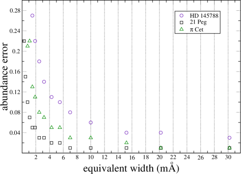
Figure 5: Error bar in abundance as a function of equivalent widths for HD 145788 (open circle), 21 Peg (open square), and $\pi$ Cet (open triangle). This uncertainty stems from the uncertainty in the equivalent-width measurement and continuum normalisation. The difference in uncertainty between 21 Peg and $\pi$ Cet comes almost only from the difference in ${\upsilon}\sin i$, while the high error obtained for HD 145788 mainly from the low SNR of our observations, relative to one of the other two stars.

The mean equivalent width measured in these three stars is about 20 mÅ for HD 145788, 5 mÅ for 21 Peg, and 8 mÅ for $\pi$ Cet. These values correspond to an error bar in abundance, because of the uncertainty on the equivalent widths measurement and continuum normalisation of 0.04 dex for HD 145788, and 0.03 dex for both 21 Peg and $\pi$ Cet.

When we have enough measured lines, we assume that the internal scatter for each ion also takes the errors due to equivalent widths measurement and continuum normalisation into account.

Figure 6 shows the abundance scatter as a function of the number of measured lines for 21 Peg. For elements where non-LTE effects are supposed to be important and line-dependent, such as Al and S, the internal standard deviation is particularly high. The same is found for elements with lower accuracy in log$gf$ values due to the complexity of the atomic levels, such as Si. For other elements with a large enough number of spectral lines, say $n>10$, it is reasonable to expect an internal error of 0.11 dex (see Fig. 6).

Considering the errors in oscillator strengths determination (see Table LABEL:line_abund) given for the laboratory data, we may say that these errors are smaller for most elements than the internal scatter, so do not significantly influence the final results. The same is relevant for theoretical calculations. As already shown for Cr ii and Fe ii (Sect. 4.1.8), calculated and laboratory sets of oscillator strengths agree within 0.1 dex.

It should be noted that error due to the internal scatter is just a part of the total error bar on the abundance determination. To derive a more realistic abundance uncertainty we also have to take the error bar due to systematic uncertainties in the fundamental parameters into account.

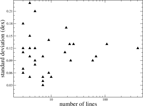
Figure 6: Standard deviation of the derived abundances as a function of the the number of lines (shown in logarithmic scale and for a number of lines greater than 2). For visualisation reasons we omitted the standard deviation given by Zr ii.

For a detailed discussion of the abundance error bars we again use 21 Peg. Table 5 shows the variation in abundance for each analysed ion, caused by the change of one fundamental parameter by $+1\sigma$, keeping fixed the other parameters. For the comparison $\sigma_{\rm abn}^{2}$ (syst.) with $\sigma_{\rm abn}$ (scatt.) of those ions for which the internal scattering could not be measured, an a priori scatter of $\sigma_{\rm abn}\,{\rm(scatt.)}=0.11$ dex has to be assumed.

Table 5: Error sources for the abundances of the chemical elements of 21 Peg.

Ion	abundance	$\sigma_{\rm abn}$ (scatt.)	$\sigma_{\rm abn}$ ($T_{\mathrm{eff}}$)	$\sigma_{\rm abn}$ ($\log g$)	$\sigma_{\rm abn}$ ($\upsilon_{\mathrm{mic}}$)	$\sigma_{\rm abn}$ (syst.)
	$\log(N/N_{\rm tot})$	(dex)	(dex)	(dex)	(dex)	(dex)
He i	$-$1.11	0.04	$-$0.08	0.03	0.00	0.09
C i	$-$3.66	0.14	$-$0.05	$-$0.13	$-$0.10	0.17
C ii	$-$3.65	0.05	$-$0.17	$-$0.02	$-$0.08	0.19
N i	$-$3.95	0.12	$-$0.05	$-$0.07	$-$0.05	0.10
N ii	$-$3.90:		$-$0.09	0.05	0.00	0.10
O i	$-$3.28	0.11	0.00	$-$0.02	$-$0.02	0.03
Ne i	$-$3.76	0.05	$-$0.18	$-$0.03	$-$0.06	0.19
Na i	$-$5.60		0.04	$-$0.04	$-$0.01	0.06
Mg i	$-$4.42	0.12	0.10	$-$0.06	$-$0.05	0.13
Mg ii	$-$4.56	0.03	$-$0.02	$-$0.01	$-$0.02	0.03
Al i	$-$5.89		0.10	$-$0.03	0.00	0.10
Al ii	$-$5.68	0.10	$-$0.09	0.01	$-$0.03	0.10
Si i	$-$4.95		0.10	$-$0.02	0.00	0.10
Si ii	$-$4.49	0.13	$-$0.07	0.01	$-$0.03	0.08
Si iii	$-$4.26	0.18	$-$0.16	0.04	$-$0.03	0.17
P ii	$-$6.37	0.06	$-$0.08	0.02	$-$0.02	0.08
S ii	$-$4.86	0.13	$-$0.14	0.00	$-$0.05	0.15
Ca i	$-$5.84	0.11	0.20	$-$0.07	0.00	0.21
Ca ii	$-$5.98	0.08	0.03	$-$0.05	$-$0.04	0.07
Sc ii	$-$9.37	0.10	0.12	$-$0.01	0.00	0.12
Ti ii	$-$7.23	0.09	0.08	0.00	$-$0.02	0.08
V ii	$-$7.98	0.06	0.06	0.02	0.00	0.06
Cr i	$-$6.29	0.09	0.13	$-$0.03	0.00	0.13
Cr ii	$-$6.20	0.10	0.03	0.02	$-$0.01	0.04
Mn i	$-$6.54	0.21	0.14	$-$0.03	0.00	0.14
Mn ii	$-$6.51	0.17	0.01	0.01	$-$0.01	0.01
Fe i	$-$4.52	0.13	0.11	$-$0.03	0.00	0.11
Fe ii	$-$4.50	0.12	$-$0.02	0.02	$-$0.02	0.03
Fe iii	$-$4.60	0.06	$-$0.10	0.06	$-$0.01	0.12
Co ii	$-$6.75	0.18	0.01	0.03	0.00	0.03
Ni i	$-$5.71	0.05	0.09	$-$0.03	$-$0.01	0.10
Ni ii	$-$5.61	0.09	$-$0.04	0.03	$-$0.01	0.05
Zn i	$-$6.86		0.10	$-$0.02	0.00	0.10
Sr ii	$-$9.10	0.01	0.13	$-$0.03	$-$0.06	0.15
Y ii	$-$9.76	0.15	0.13	$-$0.02	$-$0.01	0.13
Zr ii	$-$9.48	0.28	0.11	0.00	0.00	0.11
Ba ii	$-$9.19	0.06	0.14	$-$0.02	$-$0.01	0.14
Nd iii	$-$10.09	0.07	0.04	0.04	0.00	0.06

Column 3 standard deviation $\sigma_{\rm abn}$ (scatt.) of the mean abundance obtained from different spectral lines (internal scattering); a blank means that the number of spectral lines is $<3$, hence no internal scattering could be estimated. (Note that these values are identical to those given in Table 4.) Columns 4, 5, and 6 give the variation in abundance estimated by increasing $T_{\mathrm{eff}}$ by 200 K, $\log g$ by 0.1 dex, and $\upsilon_{\mathrm{mic}}$ by 0.4 km s^-1, respectively. Column 7 gives the the mean error calculated applying the standard error propagation theory on the systematic uncertainties given in columns 4, 5 and 6, i.e., $\sigma_{\rm abn}^{2}$ (syst.) = $\sigma_{\rm abn}^{2}$ ($T_{\mathrm{eff}}$) + $\sigma_{\rm abn}^{2}$ ($\log g$) + $\sigma_{\rm abn}^{2}$ ($\upsilon_{\mathrm{mic}}$).

The main source of uncertainty is the error in the effective temperature determination, while the variation due to $\log g$ and, in particular, to $\upsilon_{\mathrm{mic}}$ is almost negligible, although here we are considering an uncertainty on $\upsilon_{\mathrm{mic}}$ of 2$\sigma$. The abundance variation due to an increase in $\log g$ leads to a worse ionisation equilibrium for many elements for which the equilibrium is reached at the adopted $\log g$, such as Cr, Mn, Fe, and Ni. We repeated the same analysis for Fe ii for HD 145788 and $\pi$ Cet. The results are comparable with those obtained for 21 Peg. We also expect the same effect for the other ions.

Assuming the different errors in the abundance determination are independent, we derived the final error bar using standard error propagation theory, given in column six of Table 5. When the abundance is given by a single line, we assumed an internal error of 0.11 dex. Using the propagation theory we considered the situation where the determination of each fundamental parameter is an independent process. The mean value of the LTE uncertainties given in column six of Table 5 is 0.16 dex.

Because of the high SNR of the observations, the low ${\upsilon}\sin i$ and the non peculiarity of the programme stars, we can reasonably believe that the errors in abundance determinations estimated in the present study are the smallest ones that could be obtained with the current state of the art of spectral LTE analysis for early-type stars. In the cases of stars with ${\upsilon}\sin i$ higher than those considered in this work, the uncertainty on the abundances increases. A higher rotational velocity would force the abundance analysis to be based on strong and saturated lines that are more sensitive to $\upsilon_{\mathrm{mic}}$ variations than weak lines. For a more detailed discussion, see Fossati et al. (2008).

4.3 Comparison with previous abundance determinations

Table 6 (online) collects all previous massive abundance determinations in the atmosphere of 21 Peg (Sadakane 1981; Smith & Dworetsky 1993; Smith 1993, 1994; Dworetsky & Budaj 2000) in comparison with the results of the current analysis. We do not include works that only give abundances for a Cr and/or Fe.

The main advantage of our analysis over the previous ones is the wide wavelength coverage and the high quality of our spectra. It allows us to use many more spectral lines including very weak ones of the species not analysed before. Our analysis provides homogeneous abundance data for 38 ions of 26 chemical elements from He to Nd.

Reasonably good agreement exists between our abundances derived with the spectra in optical and IR spectral regions and those derived with the UV observations (Smith & Dworetsky 1993; Smith 1993, 1994), supporting the correctness of the adopted model atmosphere.

Dworetsky & Budaj (2000) derived the LTE neon abundance and gave non-LTE abundance corrections for the strongest Ne i $\lambda$ 6402 line. If we apply the non-LTE correction described in Sect. 4.1.3 to this line, we almost get the same non-LTE abundance.

For $\pi$ Cet the number of abundance determinations in the literature is particularly vast. As for 21 Peg we consider only those where abundances are derived for large number of ions: Adelman (1991), Smith & Dworetsky (1993), Smith (1993), Smith (1994), and Acke & Waelkens (2004), except for neon abundance where we again included LTE and non-LTE results by Dworetsky & Budaj (2000). For the comparison (see the online Table 7) of the abundances obtained for $\pi$ Cet, we also show the adopted $\upsilon_{\mathrm{mic}}$ because we believe that differences in this parameter are responsible for the difference between our abundances and those of Acke & Waelkens (2004). Again, we emphasise that the total number of ions (36) and elements (22), as well as the number of lines per ion analysed in the present work, is much higher than in any previous study. For Al, Si, Fe, we managed to derive abundances from the lines of the element in three ionisation stages, which provides a unique possibility to study non-LTE effects.

For the ions having several lines (S ii, Ti ii, Cr ii and Fe ii) we generally get a good agreement among the different authors, in particular, for Fe ii. The lower abundances given by Acke & Waelkens (2004) are due to the high $\upsilon_{\mathrm{mic}}$ adopted.

The difference in He abundance between our work and that by Adelman (1991) may be explained by the difference in $T_{\mathrm{eff}}$, already discussed in Sect. 3.4. Both LTE and non-LTE neon abundances agree rather well with the results by Dworetsky & Budaj (2000) after applying the non-LTE corrections given by these authors.

5 Discussion

In Fig. 7 we show the derived abundances normalised to solar values (Asplund et al. 2005). In the following, we discuss the stars of our sample individually.

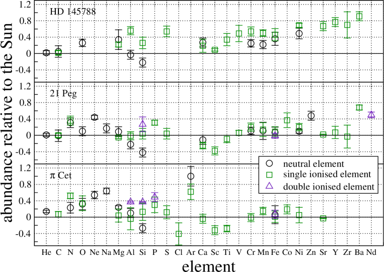
Figure 7: LTE abundances relative to the Sun (Asplund et al. 2005) for HD 145788, 21 Peg, and $\pi$ Cet, from top to bottom. The open circles, squares, and triangles indicate the abundance for the neutral element, single ionised, and double ionised, respectively. The possible non-LTE corrections for each ion are described in the text from Secs. 4.1.1 to 4.1.10.

5.1 HD 145788

HD 145788 shows a slight overabundance for almost all ions and typical Am abundance pattern for elements heavier than Ti. The overall overabundance and the Am abundance pattern could be explained if HD 145788 was formed in a region of the sky with a metallicity higher than the solar region. To be able to check the possible Am classification of HD 145788, we can compare the obtained abundance pattern with the typical one for Am stars in clusters having enhanced metallicity, e.g. the Praesepe open cluster with an overall metallicity of [Fe/H]=0.14 dex (Chen et al. 2003). Fossati et al. (2007) give the abundance pattern of eight Am stars belonging to the Praesepe cluster. All these stars show clear Am signatures: underabundances of CNO and Sc, and overabundances of the elements heavier than Ti. In HD 145788 the underabundances of CNO and Sc are not visible. For this reason we believe that the star cannot be classified as a hot Am star and that the observed abundance pattern stems from the composition of the cloud where HD 145788 was formed.

Table 4 and Fig. 7 show that with the adopted fundamental parameters of HD 145788 we get ionisation imbalance for the Fe-peak elements. With a small adjustment of the parameters within the error bars ($T_{\mathrm{eff}}$: +100 K, $\log g$: $-$0.05) it is possible to compensate for this imbalance for the Fe-peak elements, but the ionisation balance becomes worse for other elements such as C, Mg, and Ca. This is a clear sign that a non-LTE analysis is needed for this object to understand whether the ionisation violation stems from non-LTE effects or to some other physical effect. Unfortunately we cannot be completely certain of the adopted parameters because of the lack of spectrophotometric measurements.

5.2 21 Peg

The star 21 Peg shows solar abundances for almost all elements. At the temperature of 21 Peg, slowly rotating stars are usually hot Am, cool HgMn, or magnetic stars.

The possibility of classifying 21 Peg as an Am star (which is potentially suggested by the observed Sc underabundance) is excluded by the solar abundances of all the other mentioned indicators. As explained in Sect. 4.1.5, the non-LTE correction for Ca is expected to be positive, increasing the Ca abundance to the solar value, but detailed non-LTE analysis should be performed for a more accurate determination. Almost nothing is known about non-LTE effects for Sc at these temperatures, so that to understand whether the observed underabundance is real, a non-LTE analysis should be performed.

Caliskan & Adelman (1997), Adelman (1998), Adelman (1999), and Kocer et al. (2003) have published abundances of several chemically normal, early-type stars. The derived Sc abundance for stars with an effective temperature similar to that of 21 Peg is almost always below the solar value, with nearly solar abundances for other Fe-peak elements. We thus conclude that the observed abundances of most elements but Ba in 21 Peg allow us to classify it as a normal early-type rather than Am star. Solar Mn abundance and the absence of Hg ii $\lambda$3984 Å line exclude any classification of 21 Peg as an HgMn star.

5.3 $\pi$ Cet

The star $\pi$ Cet shows solar abundances for almost all elements. Only O, Ne, Na and Ar are clearly overabundant. For Ne or Na this most probably comes from non-LTE effects. For argon, the non-LTE effects are expected to be weak (see Sect. 4.1.3). In other chemically normal, early-type stars the Ar abundance appears to be above the solar one (see Lanz et al. 2008; Fossati et al. 2007; Adelman 1998), leading to the conclusion that indirect solar Ar abundance given by Asplund et al. (2005) is underestimated.

As for 21 Peg, the Sc underabundance of $\pi$ Cet is not an indication of a possible Am peculiarity. The absence of magnetic field or of normal Mn abundance, including no trace of any Hg signature in the spectrum exclude a classification of the star as magnetic peculiar or non-magnetic HgMn object.

The star $\pi$ Cet is a known binary with a period of about 7.5 years (Lacy et al. 1997) and is a Herbig AeBe star (Malfait et al. 1998). The Herbig classification comes from a detected infrared excess at wavelengths longer than 10 $\mu$m. The two spectra obtained with ESPaDOnS show variability in the line profiles, small emission-like features close to the core of H$\alpha$, and emission features at the position of C i $\lambda\lambda$ $\sim$ 8335 and 9405 Å in the near infrared. The width of C i emission lines are exactly the same as expected for absorption line in $\pi$ Cet. The pre-main-sequence status of this star, which is very likely responsible for these emissions, might also explain the variability observed in the spectral lines, as circumstellar absorption or emission coming from a proto-planetary disk. The variation in the line profile within one day excludes the possibility that the observed changes are caused by the companion.

Another explanation for the line variations comes from pulsation. We performed a frequency analysis of the radial velocity measurements given by Lacy et al. (1997) and the ones obtained from the two ESPaDOnS spectra. Preliminary results show that two frequencies appear in the amplitude spectrum: one corresponding to the orbital period and another one at $\sim$2.79 day^-1. This frequency is consistent with the expected pulsation periods for SPB stars with effective temperature of $\pi$ Cet (see Fig. 5 of Pamyatnykh 1999). In this way pulsation could explain the line-profile variation, while the presence of a disk around the star could explain the small emission visible in H$\alpha$. The C i emission lines in the near infrared could be explained either by the disk or by non-LTE effects (Nieva & Przybilla 2008).

Only future photometric observations and time-resolved spectroscopy and non-LTE analysis could lead to a better understanding of the star’s status.

6 Conclusions: are solar abundances also a reference for early A- and late B-type stars?

One of the main goal of this work was to check whether the solar abundances can be taken as a reference for early-type stars. The same question has recently been discussed by Przybilla et al. (2008) who analysed a sample of early B-type stars in the solar neighbourhood to compare the obtained non-LTE abundances with the ones published by other authors for stars in the Orion nebula, various B-type stars, young F- and G-type stars, the interstellar medium, and the sun (Grevesse et al. 1996; Asplund et al. 2005), and to check the chemical homogeneity of the solar neighbourhood. They obtained an excellent agreement between the non-LTE abundances for He, C, N, Mg, Si, and Fe with the solar ones published by Asplund et al. (2005), while the oxygen abundance lies between the solar values obtained by Grevesse et al. (1996) and Asplund et al. (2005), and the Ne abundance is compatible with the one provided by Grevesse et al. (1996).

The optical spectra of early B-type stars cannot provide reliable data for many other elements (Ca, Ti, Cr, Mn, Sr, Y, Zr), which are important for comparative abundance studies of chemically peculiar stars. While early A- and late B-type stars, investigated in the present paper, provide us with the abundances of up to 26 elements, most of which are based on enough spectral lines with accurately known atomic parameters. Figure 7 shows almost solar abundances for many elements in both 21 Peg and $\pi$ Cet, while the observed abundance pattern in HD 145788 gives a hint that the star may have been formed in a region of the sky at high metallicity. In early-type stars it is possible to directly derive the He abundance, while for the Sun it is only possible through astroseismological observations and modelling. For this reason it is important to check that the He abundance is comparable to the solar value in several chemically normal early-type stars.

In the analysed stars, several elements (He, C, Al, S, V, Cr, Mn, Fe, Ni, Sr, Y, Zr) show abundances compatible with the revised solar data (Asplund et al. 2005), and when discrepancies are present they could be explained by non-LTE effects (N, Na, Mg, Si, Ca, Ti, Nd). For Ne and Ar the expected non-LTE corrections would lead to abundances close to those derived for early B-type stars (Lanz et al. 2008; Przybilla et al. 2008) or to the solar ones given by Grevesse et al. (1996) instead of Asplund et al. (2005). Non-LTE corrections were never calculated and should be determined for other elements that show differences with the solar abundance (P, Cl, Sc, Co). We found actual discrepancies with the solar abundance for oxygen in $\pi$ Cet and for Ba in 21 Peg. While the oxygen problem may be solved by careful non-LTE analysis of all the available lines including the red and IR ones, the Ba overabundance cannot be explained by the current non-LTE results. The abundances obtained in this work for this set of three early B-type stars agree very well with the ones obtained by Przybilla et al. (2008) for all the elements.

The published abundances of Ba in chemically normal early-type stars (Lemke 1990; Caliskan & Adelman 1997; Adelman 1999; Kocer et al. 2003) show a definite trend towards a Ba overabundance. The non-LTE corrections for Ba should be positive, leading to an even greater discrepancy with the solar value, that probably does not represent early-type stars.

Non-LTE effects are studied mainly in solar-type stars, low-metallicity stars, and giants, and in stars hotter than early B-type, where the effects are expected to be strong. Very few analyses have been performed for normal early A- and late B-type stars (e.g. Vega), and our study claims the real need of such analyses for many elements before making a definite conclusion about the solar abundances as standards for early-type stars.

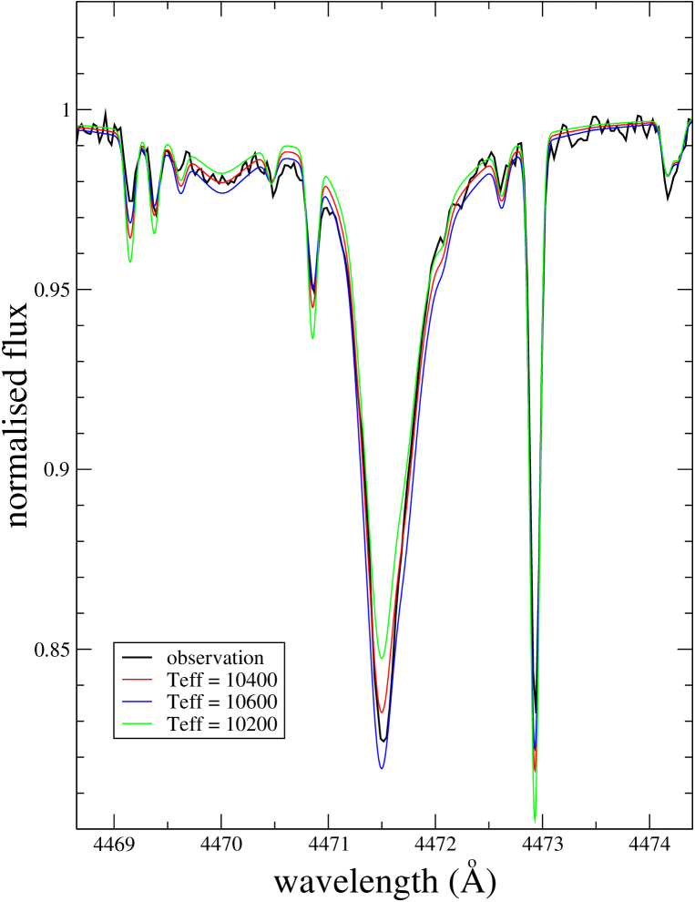
Figure 12: Comparison between the observed spectrum of the He i line at $\lambda\sim$4471 Å for 21 Peg (black thick line) and three synthetic profiles calculated with three different $T_{\mathrm{eff}}$ for the model atmosphere: 10200 K (green line), the adopted 10400 K (red line) and 10600 K (blue line).

Table 6: Comparison of the derived abundances with previous determinations for 21 Peg.

Ion	R08		S81		S934		D00
	$\log(N/N_{\rm tot})$	$n$	$\log(N/N_{\rm tot})$	$n$	$\log(N/N_{\rm tot})$	$n$	$\log(N/N_{\rm tot})$
He i	$-$1.11$\pm$0.04	7
C i	$-$3.66$\pm$0.14	9	-3.88	2
C ii	$-$3.65$\pm$0.05	4
N i	$-$3.95$\pm$0.12	4
N ii	$-$3.90:	1
O i	$-$3.28$\pm$0.11	18
Ne i	$-$3.76$\pm$0.05	7					-3.60$\pm$0.16	3
	-3.89 (non-LTE)	1					-3.82 (non-LTE)	1
Na i	$-$5.60:	1
Mg i	$-$4.42$\pm$0.12	5
Mg ii	$-$4.56$\pm$0.03	7	-4.72$\pm$0.13	7	-4.34$\pm$0.05	4
Al i	$-$5.89	2	-6.05	2
Al ii	$-$5.70$\pm$0.10	4			-5.84	1
Al iii					-5.89$\pm$0.21	2
Si i	$-$4.95:	1
Si ii	$-$4.49$\pm$0.13	22	-4.85	2	-4.63$\pm$0.07	2
Si iii	$-$4.26:	2
P ii	$-$6.37$\pm$0.06	3
S ii	$-$4.86$\pm$0.13	26
Ca i	$-$5.84$\pm$0.11	3	-5.76	1
Ca ii	$-$5.98$\pm$0.08	5	-6.24	1
Sc ii	$-$9.37$\pm$0.10	7	-9.47	3
Ti ii	$-$7.23$\pm$0.09	59	-7.15$\pm$0.16	26
V ii	$-$7.98$\pm$0.06	9	-7.78$\pm$0.16	6
Cr i	$-$6.29$\pm$0.09	5
Cr ii	$-$6.20$\pm$0.10	68	-6.39$\pm$0.25	17	-6.30$\pm$0.01	5
Mn i	$-$6.54$\pm$0.21	5	-6.08	2
Mn ii	$-$6.51$\pm$0.17	19			-6.39$\pm$0.10	3
Fe i	$-$4.52$\pm$0.13	108	-4.80$\pm$0.21	32
Fe ii	$-$4.50$\pm$0.12	406	-4.79$\pm$0.18	23	-4.59$\pm$0.05	10
Fe iii	$-$4.60$\pm$0.06	3
Co ii	$-$6.75$\pm$0.18	3			-6.01$\pm$0.01	3
Ni i	$-$5.71$\pm$0.05	10
Ni ii	$-$5.61$\pm$0.09	23	-6.13	5	-5.70$\pm$0.02	4
Zn i	$-$6.96:	1			-7.29$\pm$0.11	3
Sr ii	$-$9.10:	2	-9.18	2
Y ii	$-$9.76$\pm$0.15	4	-9.27	1
Zr ii	$-$9.48$\pm$0.28	4	-9.09	1
Ba ii	$-$9.19$\pm$0.06	3
Nd iii	$-$10.09$\pm$0.07	3

In column 2, the meaning of a colon is the same as in Table 4.

R08: this work; S81: Sadakane (1981); S934: Smith & Dworetsky (1993); Smith (1993, 1994); D00: Dworetsky & Budaj (2000).

Table 7: Comparison of the derived abundances with previous dterminations for $\pi$ Cet.

Ion	R08		A91		S934		D00		A04
	$\log(N/N_{\rm tot})$	$n$	$\log(N/N_{\rm tot})$	$n$	$\log(N/N_{\rm tot})$	$n$	$\log(N/N_{\rm tot})$	$n$	$\log(N/N_{\rm tot})$	$n$
He i	-0.97$\pm$0.04	6	-1.11$\pm$0.06	6
C ii	-3.58$\pm$0.07	7	-3.81$\pm$0.07	4
N i	-4.03$\pm$0.13	10
N ii	-3.74$\pm$0.07	9	-3.92$\pm$0.15	3
O i	-3.06$\pm$0.14	9	-3.34	2					-3.29$\pm$0.03	4
O ii	-3.04:	2
Ne i	-3.66$\pm$0.09	20					-3.71$\pm$0.19	6
	-3.86 (NLTE)	1					-3.86 (NLTE)	1
Na i	-5.23$\pm$0.07	3
Mg i	-4.27:	2	-4.88	1
Mg ii	-4.47$\pm$0.16	10	-4.56$\pm$0.08	7	-4.28$\pm$0.05	4			-4.57$\pm$0.02	4
Al i	-5.57:	2	-5.85	2
Al ii	-5.73$\pm$0.27	8			-6.04	1
Al iii	-5.30$\pm$0.02	3	-5.36	1	-5.79$\pm$0.10	2
Si i	-4.80:	1
Si ii	-4.41$\pm$0.20	31	-4.56$\pm$0.12	5	-4.44$\pm$0.05	2			-4.44$\pm$0.28	4
Si iii	-4.16:	2	-4.99	1
P ii	-6.38$\pm$0.19	9
P iii	-6.19:	1
S ii	-4.78$\pm$0.16	31	-4.86$\pm$0.18	18					-4.90	1
Cl ii	-6.95:	2
Ar i	-4.86:	2
Ar ii	-5.24$\pm$0.19	6
Ca ii	-5.77:	2	-5.72	1
Sc ii	-9.31:	1
Ti ii	-7.42$\pm$0.08	11	-7.17$\pm$0.24	14					-7.23$\pm$0.13	7
Cr ii	-6.41$\pm$0.10	21	-6.58$\pm$0.19	15	-6.00$\pm$0.2	5			-6.58$\pm$0.08	10
Mn ii	-6.50$\pm$0.09	3			-6.44$\pm$0.05	3
Fe i	-4.53$\pm$0.22	7
Fe ii	-4.58$\pm$0.14	186	-4.66$\pm$0.20	59	-4.55$\pm$0.05	10			-4.78$\pm$0.19	29
Fe iii	-4.52$\pm$0.10	4	-4.82	1
Co ii	-6.93:	1			-6.30$\pm$0.1	3
Ni ii	-5.76$\pm$0.19	17	-6.02	3	-5.80$\pm$0.2	4			-5.89$\pm$0.02	2
Sr ii	-9.15:	2
	$\upsilon_{\mathrm{mic}}$ = 1 $\mathrm{km\,s}^{-1}$		$\upsilon_{\mathrm{mic}}$ = 0 $\mathrm{km\,s}^{-1}$		$\upsilon_{\mathrm{mic}}$ = 0 $\mathrm{km\,s}^{-1}$				$\upsilon_{\mathrm{mic}}$ = 3 $\mathrm{km\,s}^{-1}$

In column 2, the meaning of a colon is the same as in Table 4.

R08: this work; A91: Adelman (1991); S934: Smith & Dworetsky (1993); Smith (1993, 1994); D00: Dworetsky & Budaj (2000); A04: Acke & Waelkens (2004)

Table 8: A collection of the experimental and theoretical transition probabilities and Stark widths for the observed Si ii lines. Errors are given in parenthesis.

Wavelength	$\chi_{\mathrm{excit}}$		log$gf$							$\log\,\gamma_{\rm St}$
Å	eV	NIST	Barach	SG	BBCB	BBC	Math	Wilke	AJPP	Wilke	LDA
3853.665	6.858	-1.341		-1.32(06)	-1.52	-1.39(06)	-1.28(05)	-1.53(11)	-1.44	-5.12	-5.15
3856.018	6.859	-0.406		-0.34(06)	-0.56	-0.43(05)	-0.36(06)	-0.65(10)	-0.49	-5.15	-5.15
3862.595	6.858	-0.757		-0.83(06)	-0.82	-0.80(06)	-0.80(07)	-0.92(10)	-0.75	-5.14	-5.15
4072.709	9.837	-2.700		-2.37(05)			-2.70(10)	-2.40(16)	-1.89	-4.89	-4.76
4075.452	9.839	-1.403		-1.40(05)			-1.40(10)	-1.64(16)	-0.95	-4.89	-4.76
4076.780	9.837	-1.700		-1.67(05)			-1.70(10)	-1.75(16)	-1.20	-4.89	-4.76
4128.054	9.837	0.359		0.45(04)	0.32		0.36(12)	0.22(08)	0.38	-4.92	-4.88
4130.872	9.839	-0.783			-0.82				-0.77		-4.88
4130.894	9.839	0.552		0.50(04)	0.48		0.55(12)	0.38(08)	0.53	-4.93	-4.88
4190.707	13.492						-0.17(10)	-0.33(11)	-0.35	-5.25	-5.26
4198.134	13.487						-1.46(11)	-0.60(11)	-0.61	-5.26	-5.26
4200.658	12.525	-0.889									-3.43
4621.418	12.525	-0.608									-3.69
4621.722	12.526	-0.453									-3.69
5041.023	10.067	0.029		0.29(03)		0.09(04)	0.03(07)	0.18(03)	0.19	-4.84	-4.78
5055.983	10.074	0.523		0.59(03)		0.46(04)	0.52(08)	0.48(03)	0.44	-4.79	-4.78
5056.316	10.074	-0.492		-0.36(03)		-0.49(04)			-0.51	-4.79	-4.78
5466.460	12.525	-0.237									-3.99
5469.451	12.880	-0.762
5540.807	14.489		-0.83(08)				-1.20(10)		-0.80
5576.661	14.504		-0.47(08)				-0.47(10)	-0.62(13)	-0.49	-5.46
5632.966	14.186	-0.818	-0.62(08)			-0.82(06)		-0.82(09)	-0.69	-5.44
5639.477	14.528		-0.07(06)			-0.30(07)	-0.07(12)	-0.18(09)	-0.32	-5.44
5669.563	14.200	0.286	0.32(06)			0.28(07)		0.12(08)	0.25	-5.53
5688.817	14.186	0.126	0.08(06)			0.13(06)		0.00(09)	0.08	-5.50
5701.370	14.175	-0.057	-0.10(06)			-0.06(07)		-0.28(09)	-0.10	-5.53
5800.454	14.504		-0.04(08)			-0.16(07)	-0.12(12)	-0.16(11)	-0.17	-5.37
5806.731	14.489		-0.10(08)			-0.13(07)	-0.11(12)	-0.18(10)	-0.20	-5.47
5827.752	14.489		-0.91(18)			-0.79(07)	-1.00(10)	-1.16(11)	-0.90	-5.45
5846.121	14.504		-0.51(08)			-0.29(07)	-0.57(12)	-0.33(14)	-0.70	-5.35
5867.480	14.504								-0.20
5868.443	14.528		0.42(06)				0.40(14)	0.50(11)	0.20	-5.36
5957.559	10.067	-0.225		-0.30(02)		-0.22(03)		-0.29(06)	-0.33	-5.02	-4.84
5978.930	10.074	0.084		0.00(02)		0.08(03)		0.03(06)	-0.03	-5.01	-4.84
6347.109	8.121	0.149		0.18(05)	0.30	0.20(04)	0.12(07)	0.29(08)	0.17	-5.31	-5.05
6371.371	8.121	-0.082		-0.06(05)	-0.00	-0.03(03)	-0.04(07)	-0.02(08)	-0.13	-5.32	-5.05
6660.532	14.504	0.162						0.23(09)	0.24	-5.51
6665.030	14.495	-0.240						-0.18(09)	-0.16	-5.54
6671.841	14.528	0.409				0.41(07)		0.46(09)	0.52	-5.58
6699.431	14.495	-0.247				-0.25(08)			-0.16
7848.816	12.525	0.316							0.34		-4.34
7849.618	12.526	-0.831							-0.80		-4.34
7849.722	12.526	0.470							0.50		-4.34

NIST – Kelleher & Podobedova (2008) – critical compilation; Barach – Barach (1970) – pulsed arc; SG – Schilz-Gulde (1969) – arc emission spectra; BBCB – Berry et al. (1971) – beam-foil lifetime measurements and theortical branching ratios; BBC – Blanco et al. (1995) – laser-induced plasma; Math – Matheron et al. (2001) – laser-induced plasma; Wilke – Wilke (2003) – laser-induced plasma, Stark widths, shifts and transition probabilities; AJPP – Artru et al. (1981) – theoretical calculations; LDA – Lanz et al. (1988) – Stark widths, semi-classical calculations.

Table 9: Linelist of the lines used for the abundance analysis.

Element			HD 145788		21 Peg		$\pi$ Cet
Wavelength	$\chi_{\mathrm{excit}}$	log$gf$	EQW	abundance	EQW	abundance	EQW	abundance	Ref log$gf$
Å	eV		mÅ	dex	mÅ	dex	mÅ	dex
He i
4026.1850	20.964	-2.620(005)	S	-1.13	S	-1.15			WSG
4026.1870	20.964	-1.450(005)	S		S				WSG
4026.1870	20.964	-0.700(005)	S		S				WSG
4026.1980	20.964	-1.450(005)	S		S				WSG
4026.3580	20.964	-1.320(005)	S		S				WSG
4026.1990	20.964	-0.970(005)	S		S				WSG
4026.3580	20.964	-1.320(005)	S		S				WSG
4120.8110	20.964	-1.743(041)			S	-1.05	S	-0.99	WSG
4120.8240	20.964	-1.963(041)			S		S		WSG
4120.9910	20.964	-2.433(041)			S		S		WSG
4168.9670	21.218	-2.338(005)					S	-1.01	WSG
4387.9290	21.218	-0.883(005)			S	-1.10		-0.98	WSG
4437.5510	21.218	-2.034(041)			S	-1.08	S	-0.95	WSG
4471.4690	20.964	-2.198(005)	S	-1.15	S	-1.08	S	-0.90	WSG
4471.4730	20.964	-1.028(005)	S		S		S		WSG
4471.4730	20.964	-0.278(005)	S		S		S		WSG
4471.4850	20.964	-1.028(005)	S		S		S		WSG
4471.4880	20.964	-0.548(005)	S		S		S		WSG
4471.6820	20.964	-0.898(005)	S		S		S		WSG
4713.1390	20.964	-1.233(041)	S	-1.05	S	-1.13	S	-0.99	WSG
4713.1560	20.964	-1.453(041)	S		S		S		WSG
4713.3760	20.964	-1.923(041)	S		S		S		WSG
4921.9310	21.218	-0.435(005)	S	-1.05	S	-1.10			WSG
C i
4029.4130	7.488	-2.190	5.4	-3.63					KP
4762.5282	7.483	-2.335(100)			1.92	-3.61			NIST08
4770.0263	7.483	-2.437(100)			1.77	-3.55			NIST08
4771.7458	7.488	-1.866(100)	19.0	-3.36	4.98	-3.65			NIST08
4775.8947	7.488	-2.304(100)			2.38	-3.55			NIST08
4932.0490	7.685	-1.658(041)	12.4	-3.65	2.82	-4.00			NIST08
5052.1670	7.685	-1.303(041)	22.7	-3.71	4.31	-4.16			NIST08
5380.3370	7.685	-1.616(041)	13.3	-3.64	1.48	-4.30			NIST08
6014.8342	8.643	-1.585(180)			2.10	-3.61			NIST08
7111.4694	8.640	-1.086(041)			6.06	-3.55			NIST08
7113.1790	8.647	-0.774(041)			5.03	-3.94			NIST08
7116.9879	8.647	-0.907(041)			4.59	-3.85			NIST08
7119.6572	8.643	-1.149(041)			4.60	-3.61			NIST08
C ii
3918.9702	16.332	-0.533(041)					S	-3.60	NIST08
4266.9991	18.046	0.562(068)	5.5	-3.68	11.10	-3.61	S	-3.63	NIST08
4267.2590	18.046	0.717(068)	8.3	-3.58	12.74	-3.67	S		NIST08
5145.1666	20.710	0.189(068)					2.5	-3.60	NIST08
6578.0530	14.449	-0.026(041)			S	-3.70	S	-3.60	NIST08
6582.8817	14.449	-0.328(041)			S	-3.60	S	-3.58	NIST08
7236.4158	16.333	0.298(041)					11.7	-3.64	NIST08
7237.1656	16.333	-0.656(041)					3.1	-3.45	NIST08
N i
6482.6986	11.764	-0.510(100)			3.77	-4.10			NIST08
6484.8081	11.758	-0.674(100)			4.89	-3.82			NIST08
6644.9650	11.764	-0.859(140)			2.70	-3.89			NIST08
6722.6141	11.845	-0.714(100)			2.61	-3.99			NIST08
7423.6453	10.326	-0.706(025)					7.9	-3.85	NIST08
7442.3003	10.330	-0.384(025)					11.8	-3.97	NIST08
7468.3132	10.336	-0.189(025)					17.2	-3.95	NIST08
8216.3313	10.336	0.133(025)					39.0	-4.11	NIST08
8680.2858	10.336	0.346(025)					45.9	-4.17	NIST08
8683.4050	10.330	0.086(025)					26.1	-4.28	NIST08
8686.1542	10.326	-0.305(025)					25.3	-3.91	NIST08
8703.2496	10.326	-0.322(025)					18.1	-4.07	NIST08
8711.7073	10.330	-0.234(025)					23.7	-4.02	NIST08
8718.8354	10.336	-0.335(025)					19.0	-4.03	NIST08
N ii
3994.9970	18.497	0.276(100)			S	-3.90	S	-3.85	WSG
4447.0300	20.409	0.285(068)					4.2	-3.66	WSG
4607.1494	18.462	-0.507(025)					2.6	-3.73	WF
4613.8676	18.466	-0.665(025)					1.7	-3.78	WF
4630.5432	18.483	0.094(025)					6.4	-3.79	WF
4643.0899	18.483	-0.359(025)					3.6	-3.67	WF
5005.1538	20.666	0.592(041)					3.5	-3.65	WF
5666.6274	18.466	-0.045(005)					1.9	-3.83	WF
5679.5540	18.483	0.250(005)					3.9	-3.72	WF
O i
3947.2928	9.146	-2.096(041)			S	-3.45			WF
4772.9155	10.741	-1.742(068)			4.64	-3.32			WF
4773.7553	10.741	-1.567(100)			5.26	-3.44			WF
4802.1377	10.741	-2.122(068)			2.45	-3.22			WF
4802.9775	10.741	-1.976(068)			3.11	-3.26			WF
4967.3739	10.740	-1.630(068)			5.10	-3.37			WF
4968.7935	10.741	-1.275(068)	14.9	-3.29	11.10	-3.37			WF
5019.2901	10.741	-1.871(068)			2.54	-3.43			WF
5020.2198	10.741	-1.725(068)			4.52	-3.32			WF
5330.7372	10.741	-0.870(068)			27.90	-3.28			WF
5435.1793	10.740	-1.766(068)	8.7	-2.99	4.18	-3.27	2.6	-3.23	WF
5435.7791	10.741	-1.544(068)			7.73	-3.21	6.1	-3.06	WF
5436.8588	10.741	-1.398(068)	14.7	-3.11	9.99	-3.24			WF
5512.7686	10.989	-1.942(068)					3.7	-2.78	WF
5958.3893	10.989	-1.742(068)					S	-3.11	WF
5958.5793	10.989	-1.471(068)					S		WF
6106.2650	14.047	-0.638(100)			1.70	-3.02			WF
6155.9864	10.740	-0.664(025)	46.3	-3.11	34.49	-3.22	25.5	-2.88	WF
6156.7761	10.741	-0.443(025)	65.3	-3.08	48.82	-3.20	37.4	-3.12	WF
6158.1858	10.741	-0.296(025)					45.2	-3.13	WF
6453.6065	10.740	-1.288(068)	13.8	-3.12	10.46	-3.20	8.0	-3.08	WF
6454.4462	10.741	-1.066(068)	20.0	-3.15	17.15	-3.17	11.2	-3.13	WF
O ii
4641.8102	22.979	0.054(041)					2.2	-3.08	WF
Ne i
5656.6590	18.613	-0.83(13)					1.9	-3.55	BM
5764.4190	18.555	-0.370					3.5	-3.72	L
5820.1560	18.576	-0.581					1.8	-3.79	L
5852.4880	16.848	-0.455(041)			2.36	-3.77	10.2	-3.71	NIST08
5881.8950	16.619	-0.747(041)			1.40	-3.83	9.2	-3.57	NIST08
5975.5340	16.619	-1.249(041)					2.3	-3.76	NIST08
6029.9968	16.671	-1.037(041)					4.4	-3.62	NIST08
6074.3370	16.671	-0.477(068)					10.1	-3.71	NIST08
6096.1631	16.671	-0.297(068)			3.40	-3.70	14.9	-3.63	NIST08
6143.0630	16.619	-0.098(041)			4.33	-3.76	20.2	-3.62	NIST08
6163.5940	16.715	-0.603(041)					8.4	-3.65	NIST08
6217.2810	16.619	-0.955(041)					5.1	-3.59	NIST08
6266.4950	16.715	-0.357(041)			2.08	-3.82	13.8	-3.56	NIST08
6334.4280	16.619	-0.315(041)					15.0	-3.57	NIST08
6382.9914	16.671	-0.230(041)					14.2	-3.66	NIST08
6402.2461	16.619	0.345(041)			7.26	-3.77	34.4	-3.51	NIST08
6506.5278	16.671	-0.021(041)			4.14	-3.69			NIST08
6598.9528	16.848	-0.342(041)					9.9	-3.65	NIST08
7032.4130	16.619	-0.249(041)					12.9	-3.56	NIST08
7488.8712	18.382	0.167(100)					3.6	-3.86	NIST08
7535.7739	18.382	0.04(18)					4.4	-3.62	NIST08
Na i
5688.2051	2.104	-0.450(005)			3.21	-5.60			WSM
5895.9240	0.000	-0.184(005)					24.6	-5.30	WSM
8183.2550	2.102	0.230(005)					7.6	-5.17	WSM
8194.8240	2.104	0.490(005)					11.4	-5.21	WSM
Mg i
4167.2710	4.346	-0.745(068)	36.2	-4.32					NIST08
4702.9912	4.346	-0.440(025)	48.8	-4.40	16.67	-4.53	2.4	-4.24	NIST08
5167.3208	2.709	-0.870(025)			40.42	-4.46			NIST08
5172.6841	2.712	-0.393(025)	123.9	-3.96	69.62	-4.36			NIST08
5183.6040	2.717	-0.167(005)	140.0	-3.87	85.63	-4.24	18.4	-4.29	NIST08
5528.4048	4.346	-0.498(025)	46.6	-4.32	14.39	-4.52			NIST08
Mg ii
3848.2110	8.864	-1.580(005)	S	-4.24	S	-4.58	S	-4.51	NIST08
3848.3410	8.864	-2.534(025)	S		S	-4.51	S		NIST08
3850.3860	8.864	-1.842(005)	S	-4.24	S	-4.55	S	-4.41	NIST08
4384.6372	9.996	-0.776(005)			39.51	-4.60			NIST08
4390.5718	9.999	-0.523(005)			60.83	-4.53			NIST08
4427.9941	9.996	-1.208(005)	29.8	-4.31	20.81	-4.56	19.0	-4.48	NIST08
4433.9878	9.999	-0.907(005)	42.2	-4.37	33.15	-4.56	30.4	-4.49	NIST08
6787.8550	12.085	-0.911(025)					3.5	-4.40	NIST08
7877.0540	9.996	0.391(005)					86.1	-4.26	NIST08
7896.0420	9.999	-0.308(025)					S	-4.40	NIST08
7896.3660	9.999	0.643(005)					S	-4.30	NIST08
8213.9870	9.996	-0.271(005)					48.9	-4.76	NIST08
8234.6360	9.999	0.032(005)					68.1	-4.73	NIST08
Al i
3944.0060	0.000	-0.623(068)	S	-5.70	S	-5.89	S	-5.57	SW
3961.5200	0.014	-0.323(068)	S	-5.70	S	-5.89	S	-5.57	SW
Al ii
4663.0459	10.598	-0.284(010)	32.6	-5.22	25.28	-5.60	35.1	-5.65	WSM
5593.2998	13.257	0.41(18)	11.9	-5.01	4.80	-5.83	10.0	-5.86	WSM
6226.1948	13.071	0.05(18)			2.77	-5.65	6.1	-5.73	WSM
6231.6210	13.073	-0.08(18)					S		WSM
6231.7500	13.073	0.40(18)					S	-5.80	WSM
6243.2030	13.077	-0.08(18)					S		WSM
6243.3672	13.077	0.67(18)	12.8	-5.12	8.93	-5.72	S	-5.80	WSM
7042.0830	11.317	0.35(07)					47.0	-5.28	WSM
7063.6820	11.317	-0.35(07)					15.4	-5.49	WSM
7471.4100	13.649	0.78(18)					4.3	-6.19	WSM
Al iii
4529.1890	17.818	0.671(068)					5.8	-5.28	NIST08
5696.6040	15.642	0.235(041)					3.9	-5.30	NIST08
5722.7300	15.642	-0.068(041)					2.2	-5.32	NIST08
Si i
3905.5230	1.909	-1.041(023)	S	-4.75:	S	-4.95	S	-4.80:	BL
Si ii
3853.6650	6.858	-1.341(100)	S	-4.30	S	-4.55	S	-4.50	KP08
3856.0180	6.859	-0.406(068)	S	-4.20	S	-4.40	S	-4.35	KP08
3862.5950	6.858	-0.757(068)	S	-4.16	S	-4.35	S	-4.30	KP08
4072.7090	9.837	-2.367(100)			3.44	-4.45			KP08
4075.4520	9.839	-1.403(068)	S	-4.30	S	-4.52	22.1	-4.56	KP08
4076.7800	9.837	-1.700(068)					15.3	-4.48	KP08
4128.0540	9.837	0.359(041)	S	-4.50	S	-4.52	S	-4.58	KP08
4130.8720	9.839	-0.783(140)	S	-4.45	S	-4.52	S	-4.60	KP08
4130.8940	9.839	0.552(041)	S		S		S		KP08
4190.7070	13.492	-0.350					11.8	-4.49	AJPP81
4198.1340	13.487	-0.607					8.5	-4.35	AJPP81
4200.6582	12.525	-0.889(200)			3.51	-4.73			KP08
4621.4180	12.525	-0.608(180)			7.02	-4.56			KP08
4621.7222	12.526	-0.453(180)			9.20	-4.59			KP08
5041.0239	10.067	0.029(041)	85.8	-4.06	73.29	-4.28	S	-4.29	KP08
5055.9839	10.074	0.523(041)	98.2	-4.39	86.78	-4.58	S	-4.49	KP08
5056.3169	10.074	-0.492(041)	41.4	-4.27	41.20	-4.40	S		KP08
5466.4609	12.525	-0.237(100)			10.73	-4.43			KP08
5469.4512	12.880	-0.762(180)			2.68	-4.43	6.2	-4.39	KP08
5540.8070	14.489	-0.796					1.2	-4.43	AJPP81
5576.6610	14.504	-0.493					3.7	-4.23	AJPP81
5632.9660	14.186	-0.818(068)					2.5	-4.19	KP08
5639.4771	14.528	-0.318			1.99	-4.20			AJPP81
5669.5630	14.200	0.286(025)					10.6	-4.54	KP08
5688.8170	14.186	0.126(041)					7.8	-4.56	KP08
5701.3700	14.175	-0.057(041)					6.4	-4.48	KP08
5800.4540	14.504	-0.170					4.7	-4.40	AJPP81
5806.7310	14.489	-0.203			2.63	-4.14			AJPP81
5827.7520	14.489	-0.903					2.1	-4.01	AJPP81
5846.1210	14.504	-0.699					3.7	-3.96	AJPP81
5867.4800	14.504	-0.203					6.7	-4.20	AJPP81
5868.4438	14.528	0.199			3.87	-4.30	12.9	-4.31	AJPP81
5957.5591	10.067	-0.225(025)			35.37	-4.57	60.5	-4.42	KP08
5978.9302	10.074	0.084(025)	62.8	-4.23	48.33	-4.56	74.3	-4.45	KP08
6371.3711	8.121	-0.082(068)	138.4	-4.08	110.50	-4.31			KP08
6660.5320	14.504	0.162(068)					S	-4.20	KP08
6665.0300	14.495	-0.240(068)					S	-4.30	KP08
6671.8410	14.528	0.409(025)			4.18	-4.20	14.8	-4.12	KP08
6699.4310	14.495	-0.247(041)					S	-4.20	KP08
7848.8160	12.525	0.316(041)					12.5	-4.89	KP08
7849.6180	12.526	-0.831(100)					S	-4.90	KP08
7849.7220	12.526	0.470(041)					S		KP08
Si iii
4552.6220	19.016	0.292(025)			2.70	-4.13			KP08
4567.8400	19.016	0.068(025)			1.20	-4.39	9.3	-4.16	KP08
4574.7570	19.016	-0.409(041)					4.7	-4.17	KP08
P ii
4420.7120	11.021	-0.478					2.1	-6.26	H
4602.0690	12.853	0.799(080)			1.82	-6.44	3.4	-6.56	MRB
5296.0770	10.802	-0.134			1.21	-6.33	3.2	-6.31	H
5344.7290	10.737	-0.329					1.6	-6.46	H
5409.7220	10.755	-0.368					1.2	-6.53	H
5425.8800	10.802	0.241			2.43	-6.35	5.6	-6.41	H
6034.0390	10.737	-0.209					3.7	-6.06	H
6043.0840	10.802	0.384					8.5	-6.21	H
6459.9450	10.935	0.161					1.7	-6.63	H
P iii
4222.1980	14.610	0.21(18)					1.8	-6.19	NIST08
S ii
3923.4450	16.198	0.44(20)					S	-4.83	WSM
3998.7590	16.246	0.06(20)			1.44	-5.09	7.3	-4.80	WSM
4028.7500	15.944	0.00(20)			3.22	-4.71			WSM
4142.2590	15.848	0.24(20)			3.39	-4.88			WSM
4153.0680	15.899	0.62(20)					18.9	-4.74	WSM
4162.6650	15.944	0.78(20)	8.2	-4.45	7.36	-4.89	21.4	-4.77	WSM
4230.9430	17.446	0.56					4.0	-5.11	Mult
4269.7250	16.092	-0.12(20)					5.5	-4.72	WSM
4294.4020	16.135	0.58(20)			4.71	-4.82			WSM
4463.5810	15.944	-0.02(18)			2.21	-4.63	7.2	-4.64	WSM
4486.6340	15.867	-0.40(18)					3.1	-4.75	WSM
4716.2710	13.617	-0.41(14)			3.34	-4.85	11.30	-4.76	WSM
4792.0070	16.135	-0.12(20)					2.6	-4.90	WSM
4815.5520	13.672	0.09(14)			6.21	-4.91	18.7	-4.83	WSM
4917.1980	14.003	-0.32(18)			2.34	-4.87	9.6	-4.74	WSM
4925.3430	13.584	-0.46(18)			3.86	-4.62			WSM
4942.4730	13.584	-0.96(18)					3.9	-4.77	WSM
5009.5670	13.617	-0.28(18)			2.80	-4.94	12.6	-4.72	WSM
5014.0420	14.068	0.10(18)			4.87	-4.79	16.9	-4.69	WSM
5032.4340	13.672	0.27(18)			6.32	-4.97			WSM
5103.3320	13.672	-0.11(18)			2.01	-5.21	7.1	-5.20	WSM
5201.0270	15.068	0.09(18)			1.86	-4.81			WSM
5212.6200	15.068	0.32(18)			2.46	-4.89			WSM
5320.7230	15.068	0.49(18)					13.3	-4.76	WSM
5345.7120	15.068	0.35(18)			2.89	-4.76			WSM
5428.6550	13.584	-0.13(18)			3.57	-4.78	13.3	-4.71	WSM
5432.7970	13.617	0.26(18)			5.51	-4.90			WSM
5453.8550	13.672	0.48(18)	10.9	-4.27	7.27	-4.91	28.7	-4.63	WSM
5509.7050	13.617	-0.14(18)			3.15	-4.79	11.5	-4.76	WSM
5526.2430	13.701	-0.53(18)					3.6	-5.01	WSM
5556.0230	13.617	-0.99(18)					2.6	-4.74	WSM
5564.9580	13.672	-0.32(18)					9.0	-4.70	WSM
5578.8700	13.677	-0.51(18)					4.4	-4.92	WSM
5606.1510	13.733	0.31(18)			4.31	-4.97	16.7	-4.86	WSM
5616.6330	13.660	-0.64(18)					4.2	-4.81	WSM
5639.9770	14.068	0.28(18)			4.50	-4.74			WSM
5640.3460	13.701	0.15(20)			3.60	-4.91			MWRB
5647.0200	14.003	0.04(18)			3.51	-4.68	13.0	-4.65	WSM
5664.7730	13.660	-0.25(18)			1.64	-4.94	6.9	-4.91	WSM
5819.2540	14.068	-0.76(14)					3.0	-4.64	WSM
6312.6850	14.234	-0.14(18)					3.6	-4.96	WSM
Cl ii
4794.5560	13.375	0.455(100)					0.5	-7.15	WSM
4810.0700	13.375	0.292(100)					0.8	-6.76	WSM
Ar i
8103.6920	11.624	-0.130(010)					5.6	-4.69	NIST08
8115.3110	11.548	0.360(010)					8.2	-5.03	NIST08
Ar ii
4277.5280	18.454	-0.060(041)					1.0	-5.04	NIST08
4426.0010	16.749	0.158(005)					2.2	-5.37	NIST08
4430.1890	16.813	-0.174(041)					1.9	-5.09	NIST08
4609.5670	18.454	0.304(005)					1.0	-5.23	NIST08
4735.9060	16.644	-0.108(005)					1.6	-5.15	NIST08
4806.0210	16.644	0.210(005)					1.3	-5.54	NIST08
Ca i
4226.7280	0.000	0.244	62.8	-5.63	10.44	-5.95			SG
4302.5278	1.899	0.292(010)			1.40	-5.85			S
4434.9570	1.886	-0.007(020)	11.4	-5.44					SN
4454.7788	1.899	0.258(020)	17.7	-5.48	1.77	-5.72			SN
5588.7490	2.526	0.358(011)	12.9	-5.38					SR
6439.0752	2.526	0.390(010)	14.2	-5.35					SR
Ca ii
3933.6630	0.000	0.105(027)	S	-5.70	S	-5.85	S	-5.85	T
5001.4790	7.505	-0.507	23.4	-5.57	5.56	-5.99	3.6	-5.69	TB
5019.9712	7.515	-0.247	36.0	-5.54	10.14	-5.96			TB
5021.1382	7.515	-1.207	8.6	-5.38					TB
5285.2661	7.505	-1.147	10.5	-5.34	1.15	-6.05			TB
5307.2241	7.515	-0.848			2.21	-6.05			TB
6456.8750	8.438	0.405	30.0	-5.71					TB
Sc ii
4246.8218	0.315	0.242(020)	69.1	-8.92	19.40	-9.50	2.5	-9.31	LD
4294.7671	0.605	-1.391(040)			0.89	-9.17			LD
4374.4570	0.618	-0.418(074)			4.84	-9.38			LD
4400.3892	0.605	-0.536(043)	25.7	-8.87	3.95	-9.37			LD
4415.5571	0.595	-0.668(045)	19.2	-8.91	2.83	-9.39			LD
5031.0210	1.357	-0.400(047)	13.6	-8.92	1.89	-9.42			LD
5526.7900	1.768	0.024(050)	21.2	-8.87	3.31	-9.36			LD
Ti ii
4012.3835	0.574	-1.84(04)			17.99	-7.16			PTP
4028.3384	1.892	-0.96(03)			19.95	-7.24			PTP
4053.8208	1.893	-1.13(03)	49.9	-6.72	15.14	-7.23			PTP
4161.5293	1.084	-2.09(04)	22.0	-6.85	5.46	-7.24			PTP
4163.6436	2.590	-0.13(03)	73.7	-6.79	34.44	-7.30	5.8	-7.42	PTP
4171.9038	2.598	-0.29(03)	65.6	-6.82			4.5	-7.37	PTP
4174.0718	2.598	-1.26(04)	10.7	-7.17	4.54	-7.30			PTP
4287.8735	1.080	-1.79(02)	32.0	-6.94	8.99	-7.31			PTP
4290.2148	1.165	-0.85(03)	82.9	-6.70	38.52	-7.30	4.5	-7.48	PTP
4300.0420	1.180	-0.44(03)	103.5	-6.59	55.58	-7.27	10.4	-7.48	PTP
4301.9224	1.161	-1.15(03)			24.27	-7.35	2.2	-7.51	PTP
4374.8159	2.061	-1.61(03)			4.74	-7.24			PTP
4386.8467	2.598	-0.96(04)	31.4	-6.87	10.18	-7.22			PTP
4391.0249	1.231	-2.28(05)	16.2	-6.76	3.61	-7.17			PTP
4394.0586	1.221	-1.78(04)	31.6	-6.87	8.35	-7.28			PTP
4395.0312	1.084	-0.54(02)	103.8	-6.52	55.42	-7.23	11.5	-7.38	PTP
4395.8389	1.243	-1.93(04)	26.1	-6.83	7.53	-7.16			PTP
4399.7651	1.237	-1.19(03)	61.5	-6.85	24.00	-7.28			PTP
4409.5195	1.231	-1.84(08)			6.57	-7.33			PTP
4411.0723	3.095	-0.67(03)	28.7	-6.93	11.11	-7.19			PTP
4411.9292	1.224	-2.52(08)	7.7	-6.90	2.09	-7.18			PTP
4417.7134	1.165	-1.19(02)	62.7	-6.87	24.81	-7.30			PTP
4418.3311	1.237	-1.97(04)	24.0	-6.85	5.49	-7.28			PTP
4421.9385	2.061	-1.66(04)	18.3	-6.82	4.77	-7.19			PTP
4441.7290	1.180	-2.33(04)	13.2	-6.85	3.75	-7.13			PTP
4443.8008	1.080	-0.72(02)	92.7	-6.64	7.52	-7.26	7.0	-7.44	PTP
4450.4819	1.084	-1.52(02)	51.6	-6.82	16.61	-7.26			PTP
4464.4487	1.161	-1.81(02)	32.4	-6.87	9.60	-7.22			PTP
4468.5068	1.131	-0.60(02)	96.5	-6.64	51.62	-7.25			BHN
4469.1499	1.084	-2.33(05)			3.30	-7.24			PTP
4488.3247	3.124	-0.51(03)	35.5	-6.93	13.46	-7.24			PTP
4501.2700	1.116	-0.77(02)	92.7	-6.59	45.64	-7.24			PTP
4518.3315	1.080	-2.56	10.8	-6.44	2.38	-7.17			Kur00
4529.4800	1.572	-1.64(03)	29.8	-6.85					PTP
4533.9600	1.237	-0.53(02)	97.6	-6.63	51.37	-7.27			PTP
4544.0161	1.243	-2.58(07)	9.6	-6.72	1.71	-7.20			PTP
4549.6216	1.584	-0.11(03)			64.47	-7.11			PTP
4563.7573	1.221	-0.69(02)	87.7	-6.73	40.98	-7.38	5.6	-7.52	PTP
4568.3237	1.224	-2.94			1.02	-7.08			PTP
4571.9712	1.572	-0.32(03)	106.2	-6.44	56.42	-7.15	10.6	-7.41	PTP
4657.2002	1.243	-2.24(03)			3.59	-7.21			PTP
4708.6621	1.237	-2.34(05)	16.7	-6.69	2.87	-7.22			PTP
4763.8833	1.221	-2.36(06)	13.0	-6.82	2.50	-7.27			PTP
4764.5239	1.237	-2.95			1.25	-6.98			PTP
4779.9849	2.048	-1.26(05)	34.8	-6.84	10.19	-7.24	1.3	-7.22	RHL
4798.5317	1.080	-2.68(08)			2.44	-7.05			PTP
4805.0850	2.061	-0.96(06)	50.1	-6.83	17.19	-7.25			RHL
4911.1948	3.124	-0.61(03)	33.2	-6.88	10.83	-7.25			PTP
5010.2104	3.095	-1.29(06)			3.37	-7.15			PTP
5013.6860	1.582	-2.19(06)	12.2	-6.81	2.72	-7.20			PTP
5072.2866	3.124	-1.06(04)	17.7	-6.81	4.44	-7.23			PTP
5129.1562	1.892	-1.24(03)	36.3	-6.93	11.03	-7.31			PTP
5154.0679	1.566	-1.75(03)	28.3	-6.79	6.56	-7.25			PTP
5185.9019	1.893	-1.49(03)	32.7	-6.75	10.18	-7.10			PTP
5188.6870	1.582	-1.05(02)	58.7	-6.87	20.67	-7.33	2.2	-7.41	PTP
5211.5303	2.590	-1.16(05)	14.2	-7.15	3.42	-7.56			PTP
5226.5386	1.566	-1.26(02)	48.0	-6.88					PTP
5262.1411	1.582	-2.25(07)			2.64	-7.16			PTP
5268.6074	2.598	-1.67			2.34	-7.21			K00
5336.7861	1.582	-1.59(03)			8.66	-7.26			PTP
5381.0210	1.566	-1.92(05)	15.2	-6.97	4.20	-7.28			PTP
5418.7676	1.582	-2.00(05)	15.5	-6.88	3.45	-7.28			PTP
V ii
4002.9360	1.428	-1.447(041)			3.99	-7.99			BGF
4005.7050	1.817	-0.522(027)			15.73	-8.02			BGF
4023.3780	1.805	-0.689(027)	33.5	-7.64	11.23	-8.04			BGF
4035.6220	1.793	-0.767(230)	33.8	-7.56					BGF
4036.7770	1.476	-1.594(020)	7.7	-7.74	3.10	-7.94			BGF
4202.3550	1.704	-1.523(117)			2.97	-7.91			BGF
4225.2130	2.026	-1.463(032)			1.80	-8.02			BGF
4528.4850	2.276	-1.098(029)			2.72	-8.06			BGF
4564.5790	2.268	-1.393(067)	12.1	-7.27	1.88	-7.94			BGF
4600.1660	2.265	-1.523(119)			1.52	-7.91			BGF
Cr i
4274.7969	0.000	-0.231(041)	24.5	-6.15	5.40	-6.33			MFW
4289.7168	0.000	-0.361(041)	17.2	-6.23	3.29	-6.43			MFW
5204.5112	0.941	-0.208(041)	8.7	-6.19	2.30	-6.23			MFW
5206.0371	0.941	0.019(041)	18.5	-6.03	3.64	-6.25			MFW
5208.4248	0.941	0.158(041)			5.27	-6.22			MFW
Cr ii
4003.2830	6.484	-0.723			9.41	-6.33			RU
4012.4961	5.662	-1.085			17.26	-6.07			RU
4017.9629	5.330	-2.279			1.10	-6.37			RU
4037.9719	6.487	-0.679	19.5	-6.03	11.23	-6.29	3.3	-6.49	RU
4049.0969	6.484	-1.032			6.19	-6.23			RU
4051.9299	3.104	-2.360	27.4	-6.08	12.29	-6.35	2.8	-6.44	RU
4054.0759	3.105	-2.478			8.12	-6.44			RU
4056.0559	5.662	-1.812			1.87	-6.43			RU
4072.5610	3.714	-2.632			5.28	-6.17			RU
4132.4189	3.758	-2.568			5.23	-6.22			RU
4145.7808	5.319	-1.106	28.0	-6.02	15.42	-6.29			RU
4172.5908	3.105	-2.943			3.15	-6.43			RU
4179.4209	3.827	-1.996	33.5	-5.86	16.14	-6.18			RU
4195.4170	5.319	-1.753					1.5	-6.30	RU
4207.3628	3.827	-2.731			3.92	-6.15			RU
4215.7378	3.104	-3.168			3.69	-6.13			RU
4236.3789	3.104	-3.606			1.44	-6.12			RU
4242.3638	3.871	-1.363	64.8	-5.78					RU
4252.6318	3.858	-2.054	27.0	-5.93	13.03	-6.22			RU
4254.5220	5.871	-1.294			6.99	-6.23			RU
4256.1079	6.487	-1.520			2.16	-6.22			RU
4261.9131	3.864	-1.560	51.9	-5.88	30.94	-6.16	6.7	-6.48	RU
4269.2769	3.854	-2.201	22.7	-5.89	9.91	-6.22			RU
4275.5669	3.858	-1.736	42.2	-5.91	23.31	-6.19	4.4	-6.50	RU
4284.1880	3.854	-1.897	31.1	-6.00	17.13	-6.23	3.7	-6.43	RU
4306.9160	5.873	-1.602			3.93	-6.18			RU
4465.7310	6.487	-1.279			2.59	-6.38			RU
4511.7749	6.484	-1.375			2.37	-6.32			RU
4539.5952	4.042	-2.394	15.1	-5.82	5.57	-6.21	0.8	-6.53	RU
4554.9878	4.071	-1.491	49.9	-5.88	28.81	-6.17	7.3	-6.41	RU
4558.6499	4.073	-0.662	97.8	-5.54	61.28	-6.11	27.9	-6.48	RU
4565.7402	4.042	-1.982	27.0	-5.90	12.95	-6.19	3.3	-6.31	RU
4588.1992	4.071	-0.845	87.5	-5.62	54.80	-6.12	24.4	-6.39	RU
4592.0488	4.074	-1.473	53.0	-5.82	29.19	-6.17	6.7	-6.47	RU
4616.6289	4.072	-1.576	47.2	-5.85	25.53	-6.17	5.5	-6.46	RU
4618.8032	4.074	-1.084	72.1	-5.77	44.97	-6.15	15.1	-6.44	RU
4634.0698	4.072	-1.236	66.3	-5.76	38.59	-6.17	11.6	-6.43	RU
4697.5981	5.670	-1.913			2.75	-6.13			RU
4723.3398	4.168	-2.784			1.25	-6.42			RU
4736.9990	4.156	-2.872			1.39	-6.29			RU
4779.0532	5.670	-2.409			2.04	-5.77			RU
4812.3369	3.864	-2.125	24.4	-5.92	11.25	-6.22	2.2	-6.43	RU
4824.1270	3.871	-1.085			47.81	-6.18			RU
4901.6230	6.487	-1.141			5.71	-6.12			RU
4912.4619	6.484	-1.262	9.7	-5.78	4.32	-6.13			RU
4920.2300	3.887	-3.161			1.19	-6.22			RU
4952.7939	6.282	-1.573			2.85	-6.12			RU
5153.4990	3.758	-2.500	13.9	-5.92	5.66	-6.24			RU
5232.4961	4.071	-2.360	13.0	-5.91	6.30	-6.15			RU
5237.3291	4.073	-1.350	57.2	-5.85	33.00	-6.18	6.8	-6.58	RU
5243.4570	4.042	-2.764			2.28	-6.23			RU
5246.7681	3.714	-2.466	12.8	-5.93	5.85	-6.27			RU
5274.9639	4.071	-1.559	46.1	-5.87	26.66	-6.14	7.8	-6.30	RU
5279.8760	4.073	-2.112			8.64	-6.24			RU
5280.0542	4.074	-2.316			6.85	-6.15			RU
5305.8530	3.827	-2.160			10.73	-6.22			RU
5308.4082	4.071	-2.058			12.14	-6.12			RU
5313.5630	4.074	-1.779			18.36	-6.16			RU
5334.8691	4.072	-1.826			16.02	-6.19	4.1	-6.34	RU
5369.3560	3.871	-3.045			1.81	-6.14			RU
5407.6040	3.827	-2.459	14.4	-5.90	6.91	-6.14	1.1	-6.41	RU
5420.9219	3.758	-2.458	17.3	-5.74	5.74	-6.26			RU
5478.3652	4.178	-1.968	25.5	-5.85	11.92	-6.15	4.4	-6.10	RU
5502.0669	4.168	-2.117	23.1	-5.77	8.69	-6.17			RU
5508.6060	4.156	-2.252	15.4	-5.87	6.55	-6.18			RU
5620.6309	6.487	-1.395			3.40	-6.06			RU
5678.3901	6.484	-1.496			2.53	-6.10			RU
6053.4658	4.745	-2.219			3.05	-6.22			RU
6089.6318	6.487	-1.445			2.49	-6.12			RU
6129.2261	4.750	-2.511			2.01	-6.11			RU
Mn i
4030.7529	0.000	-0.470(068)			3.02	-6.81			MFW
4034.4829	0.000	-0.811(068)	10.6	-6.50	2.29	-6.60			MFW
4041.3550	2.114	0.285(068)	10.1	-6.35	2.65	-6.44			MFW
4783.4268	2.298	0.042(041)			1.99	-6.25			MFW
4823.5239	2.319	0.144(041)			1.10	-6.60			MFW
Mn ii
4200.2700	6.185	-1.741			2.06	-6.27			K88
4205.3770	1.809	-3.440(113)			4.02	-6.62			KG
4206.3672	5.397	-1.553(041)	14.2	-6.02	4.22	-6.54			KSG
4251.7168	6.185	-1.058	11.6	-6.19	4.11	-6.64	2.1	-6.52	K88
4252.9629	6.186	-1.138			4.15	-6.55			K88
4283.7690	5.373	-2.204			2.52	-6.14			K88
4292.2368	5.380	-1.544(041)	10.8	-6.18	3.22	-6.69	1.4	-6.58	KSG
4478.6372	6.645	-0.950			2.80	-6.68			K88
4518.9561	6.645	-1.329			1.81	-6.49			K88
4727.8408	5.370	-2.017			2.19	-6.38			K88
4730.3950	5.373	-2.147			2.02	-6.29			K88
4738.2900	5.380	-1.876(061)			3.11	-6.36			KSG
4755.7271	5.397	-1.242	17.4	-6.20					K88
4764.7280	5.398	-1.351			5.76	-6.58	3.1	-6.40	K88
4784.6250	6.573	-1.505			1.51	-6.42			K88
4791.7822	6.185	-1.715			1.01	-6.59			K88
4806.8232	5.418	-1.848(061)			1.75	-6.62			KSG
5559.0469	6.185	-1.318			2.72	-6.50			K88
5570.5391	6.177	-1.444			1.94	-6.53			K88
6122.4502	10.184	0.950			1.49	-6.87			K88
Fe i
3998.0527	2.692	-0.910(041)			2.91	-4.50			BWL
4005.2419	1.557	-0.610(025)			14.97	-4.62			MFW
4006.3108	3.267	-0.99(10)			1.66	-4.36			MFW
4007.2722	2.758	-1.276(037)			1.95	-4.28			BWL
4017.1484	3.047	-1.063(025)			1.72	-4.39			BWL
4021.8665	2.758	-0.729(029)	20.6	-4.16					BWL
4030.4885	3.211	-0.555(037)			2.47	-4.65			BWL
4045.8125	1.485	0.280(025)	96.1	-3.95	46.20	-4.64	7.4	-4.73	MFW
4062.4409	2.845	-0.862(045)	17.5	-4.07	2.86	-4.47			BWL
4063.2759	3.368	-0.804			1.97	-4.41			K88
4063.5942	1.557	0.062(021)	79.5	-4.20	36.30	-4.67	5.0	-4.66	BWL
4067.9778	3.211	-0.472(037)			4.77	-4.42			BWL
4071.7380	1.608	-0.022(025)			31.65	-4.68	5.5	-4.51	MFW
4132.0581	1.608	-0.675(021)			13.17	-4.60			BWL
4132.8994	2.845	-1.006(037)			1.72	-4.56			BWL
4134.6777	2.831	-0.649(045)			4.54	-4.48			BWL
4143.4146	3.047	-0.204(037)	31.3	-4.26					BWL
4143.8682	1.557	-0.511(021)	52.2	-4.37					BWL
4153.8999	3.396	-0.321(021)	18.4	-4.27	4.54	-4.50			BWL
4154.4985	2.831	-0.688(041)	14.6	-4.36	3.26	-4.60			BWL
4154.8057	3.368	-0.400(029)	18.5	-4.21	4.69	-4.42			BWL
4156.7988	2.831	-0.809(037)	15.5	-4.21					BWL
4157.7803	3.417	-0.403(021)	17.8	-4.20	2.91	-4.62			BWL
4158.7925	3.430	-0.67(10)	10.5	-4.20					MFW
4172.1221	3.251	-0.893(057)			1.96	-4.39			BWL
4175.6362	2.845	-0.827(037)	15.6	-4.18	2.73	-4.53			BWL
4181.7549	2.831	-0.371(037)	30.7	-4.23	7.88	-4.50			BWL
4187.0391	2.449	-0.548(025)	32.2	-4.25	8.66	-4.48			MFW
4191.4307	2.469	-0.666(041)	20.3	-4.41	5.22	-4.60			BWL
4196.2085	3.396	-0.696(025)	14.2	-4.04					BWL
4199.0952	3.047	0.155(037)	40.3	-4.42					BWL
4202.0293	1.485	-0.708(025)	47.6	-4.33	14.87	-4.57			MFW
4217.5454	3.430	-0.484(025)	11.3	-4.35	2.35	-4.63			BWL
4219.3604	3.573	0.000(021)	23.2	-4.35	6.66	-4.55			BWL
4222.2129	2.449	-0.967(025)	17.6	-4.21	3.52	-4.50			MFW
4224.1719	3.368	-0.506(025)	14.7	-4.23					BWL
4225.4541	3.417	-0.510(025)			2.38	-4.60			BWL
4233.6030	2.482	-0.604(025)	27.1	-4.29	6.61	-4.55			MFW
4235.9370	2.425	-0.341(025)	38.2	-4.34	11.02	-4.58			MFW
4247.4253	3.368	-0.239(037)	19.9	-4.33	4.71	-4.59			BWL
4250.1196	2.469	-0.405(025)	33.9	-4.34	9.30	-4.58			MFW
4250.7871	1.557	-0.714(021)	47.0	-4.29	12.90	-4.60			BWL
4260.4746	2.399	0.109(029)	56.3	-4.42	21.64	-4.66	2.7	-4.61	BWL,BK
4271.1538	2.449	-0.349(025)	35.8	-4.37	11.23	-4.55			MFW
4271.7607	1.485	-0.164(025)	75.4	-4.16	32.47	-4.60	3.0	-4.71	MFW
4299.2349	2.425	-0.405(021)	33.8	-4.38	8.76	-4.64			BWL
4383.5449	1.485	0.200(025)	90.5	-4.10	45.27	-4.61			MFW
4404.7505	1.557	-0.142(025)	77.1	-4.11	31.24	-4.61			MFW
4415.1226	1.608	-0.615(025)	49.4	-4.32	15.68	-4.57			MFW
4422.5679	2.845	-1.115(025)			1.77	-4.45			BWL
4442.3389	2.198	-1.255(025)	15.1	-4.16	3.31	-4.38			MFW
4443.1943	2.858	-1.043(025)			2.33	-4.39			BWL
4447.7173	2.223	-1.342(025)	14.2	-4.09					MFW
4454.3809	2.831	-1.299(025)			0.76	-4.65			BWL
4466.5518	2.831	-0.600(057)	23.4	-4.19	4.99	-4.50			BWL
4469.3755	3.654	-0.477(068)			3.44	-4.34			BWL
4482.2529	2.223	-1.482(083)			3.35	-4.13			BWL
4484.2197	3.602	-0.864(037)	10.1	-3.93	1.65	-4.31			BWL
4494.5630	2.198	-1.136(025)	18.8	-4.16	3.35	-4.50			MFW
4528.6143	2.176	-0.822(025)			6.37	-4.52			MFW
4556.1260	3.602	-0.787(029)			2.36	-4.23			BWL
4667.4531	3.602	-0.751(041)	12.8	-3.93	1.46	-4.48			BWL
4668.1318	3.266	-1.295	9.7	-3.72					K88
4678.8457	3.602	-0.833(041)	10.6	-3.94	1.36	-4.43			BWL
4707.2744	3.241	-1.08(20)	9.0	-3.98					MFW
4736.7734	3.211	-0.752(041)			2.21	-4.51			BWL
4789.6509	3.546	-0.958(037)			1.27	-4.37			BWL
4903.3101	2.882	-0.926(025)			2.36	-4.49			BWL
4918.9941	2.865	-0.342(029)	26.0	-4.37	6.71	-4.59			BWL
4920.5029	2.832	0.068(025)	47.0	-4.33	16.48	-4.55			BWL
4957.2988	2.851	-0.408(029)	20.1	-4.47	6.39	-4.56			BWL
4957.5967	2.808	0.233(021)	60.2	-4.22	21.42	-4.57			BWL
4966.0889	3.332	-0.871(061)	7.0	-4.27					BWL
4973.1021	3.960	-0.95(07)	7.9	-3.76					MFW
4982.5239	4.103	0.144	13.7	-4.49	3.19	-4.75			K88
4983.2671	4.154	-0.158	8.3	-4.41	1.95	-4.64			K88
4983.8652	4.103	-0.068	10.3	-4.43	2.90	-4.58			K88
4985.2529	3.928	-0.560(037)			1.83	-4.39			BWL
5005.7109	3.884	-0.180	17.8	-4.16	3.19	-4.54			K88
5006.1191	2.832	-0.638(025)			4.31	-4.53			BWL,BK
5007.2930	4.103	-0.210			1.55	-4.72			K88
5014.9424	3.943	-0.303(053)	9.6	-4.32	2.31	-4.54			BWL
5022.2354	3.984	-0.53(07)			1.70	-4.42			MFW
5049.8198	2.279	-1.355(029)	9.1	-4.27					BWL
5074.7485	4.220	-0.20(07)	12.0	-4.15					MFW
5125.1172	4.220	-0.14(18)	10.9	-4.26					MFW
5133.6885	4.178	0.14(18)	22.9	-4.16	5.55	-4.44			MFW
5137.3823	4.178	-0.40(07)	13.6	-3.91	2.26	-4.31			MFW
5139.2515	2.998	-0.741(025)			3.16	-4.47			BWL
5139.4629	2.940	-0.509(025)			6.76	-4.38			BWL
5162.2729	4.178	0.02(18)	18.5	-4.17	3.92	-4.48			MFW
5165.4072	4.220	-0.035	9.3	-4.44					K88
5192.3442	2.998	-0.421(025)	21.5	-4.33	5.37	-4.55			BWL
5195.4678	4.220	-0.002	10.4	-4.42					K88
5215.1807	3.266	-0.871(029)			5.50	-3.93			BK
5217.3892	3.211	-1.070(029)	8.0	-4.07					BKK
5232.9404	2.940	-0.058(021)			11.83	-4.55			BWL
5263.3062	3.266	-0.879(029)			2.61	-4.27			BKK
5266.5552	2.998	-0.386(029)	22.5	-4.33	5.62	-4.56			BWL
5269.5376	0.859	-1.321(025)	36.1	-4.36	8.37	-4.63			MFW
5281.7905	3.038	-0.834(041)	11.2	-4.24	2.16	-4.53			BWL
5283.6211	3.241	-0.432(029)	16.5	-4.32	3.52	-4.60			BKK
5324.1792	3.211	-0.103(029)			7.14	-4.60			BKK
5328.0386	0.915	-1.466(025)			6.56	-4.57			MFW
5339.9292	3.266	-0.647(029)	18.6	-4.02	3.35	-4.39			BKK
5364.8711	4.445	0.228(049)	16.0	-4.29	3.26	-4.62			BWL
5367.4668	4.415	0.443(029)	20.0	-4.39	5.23	-4.63			BWL,BK
5369.9619	4.371	0.536(021)	24.4	-4.39	5.96	-4.69			BWL
5371.4897	0.958	-1.645(025)	22.8	-4.29	4.14	-4.59			MFW
5383.3691	4.312	0.645(021)	29.9	-4.40	10.10	-4.57	3.5	-4.12	BWL
5393.1675	3.241	-0.715(029)	9.8	-4.31	2.24	-4.52			BKK
5400.5024	4.371	-0.16(18)	14.1	-4.01	2.69	-4.36			MFW
5410.9097	4.473	0.398(021)	20.3	-4.31	4.40	-4.64			BWL
5415.1992	4.386	0.642(021)	31.6	-4.32	8.21	-4.63			BWL
5424.0684	4.320	0.52(18)	33.6	-4.19	8.51	-4.53			MFW
5429.6968	0.958	-1.879(025)			3.15	-4.48			MFW
5434.5239	1.011	-2.122(025)	11.6	-4.15	1.57	-4.52			MFW
5445.0425	4.386	-0.02(18)	14.4	-4.13	2.29	-4.57			MFW
5446.9170	0.990	-1.914(025)	17.3	-4.16	2.14	-4.60			BWL
5462.9531	4.473	-0.156			2.22	-4.39			K88
5463.2764	4.434	0.11(07)			2.34	-4.66			MFW
5572.8423	3.396	-0.275(029)	19.7	-4.28	4.23	-4.57			BKK
5586.7559	3.368	-0.120(033)	24.9	-4.31					BWL,BKK
5602.9453	3.430	-0.850(029)			1.52	-4.44			BK
5615.6440	3.332	0.050(029)	27.9	-4.43	7.11	-4.69	1.4	-4.39	BKK
5862.3530	4.549	-0.058			1.81	-4.53			K88
6230.7231	2.559	-1.281(025)	9.1	-4.16	2.10	-4.34			MFW
6400.0010	3.602	-0.290(029)	15.0	-4.27	2.93	-4.58			BKK
Fe ii
3922.0040	9.126	-1.106					S	-4.54	RU
3938.9700	5.911	-1.932					S	-4.54	RU
4012.7439	10.987	-0.562			1.62	-4.80			RU
4024.5471	4.495	-2.439			30.01	-4.47			RU
4031.4419	4.732	-3.162			6.91	-4.51			RU
4041.6411	5.569	-3.376			2.65	-4.32			RU
4044.0120	5.571	-2.671					6.2	-4.39	RU
4048.8320	5.569	-2.381			16.05	-4.41	11.4	-4.38	RU
4052.4751	9.836	-1.276			1.78	-4.56			RU
4057.4610	7.274	-1.680					8.0	-4.50	RU
4060.7419	9.836	-1.416			1.41	-4.52			RU
4061.7820	5.956	-2.927	14.0	-3.75	5.17	-4.27	3.5	-4.23	RU
4138.2080	4.732	-3.494			4.74	-4.36			RU
4138.4048	2.828	-4.316			5.16	-4.48			RU
4147.2720	4.616	-3.788			2.29	-4.45			RU
4167.2990	11.196	-0.557					3.9	-4.28	RU
4173.4610	2.583	-2.617					38.4	-4.70	RU
4177.6919	2.544	-3.449			29.40	-4.51	14.5	-4.56	RU
4178.8618	2.583	-2.535	88.3	-4.14	57.71	-4.59	42.8	-4.67	RU
4182.6890	4.732	-3.960			0.96	-4.61			RU
4183.2002	2.642	-5.090			1.53	-4.36			RU
4199.4912	11.149	-0.226	9.8	-4.03			6.8	-4.37	RU
4200.5210	11.167	-0.303			2.10	-4.82			RU
4202.5220	6.807	-2.360			3.56	-4.58			RU
4202.8589	6.807	-2.665			2.45	-4.44			RU
4205.5952	11.207	-0.302			5.08	-4.38			RU
4235.3940	11.149	-0.758			2.72	-4.24			RU
4250.4370	7.684	-1.719			6.56	-4.49	5.6	-4.45	RU
4258.1538	2.704	-3.478	46.3	-4.18	21.22	-4.63			RU
4258.3398	2.642	-4.301			5.69	-4.55			RU
4263.8691	7.693	-1.691	15.1	-4.01	7.27	-4.46	6.0	-4.42	RU
4273.3262	2.704	-3.303	50.4	-4.26	27.48	-4.63	13.7	-4.67	RU
4278.1592	2.692	-3.951			13.34	-4.44			RU
4286.2798	7.708	-1.715	15.6	-3.96	8.65	-4.34	5.9	-4.42	RU
4296.5718	2.704	-2.933	65.9	-4.28	40.34	-4.65	24.9	-4.68	RU
4303.1758	2.704	-2.511			55.97	-4.61	39.9	-4.71	RU
4369.4110	2.778	-3.584					7.0	-4.70	RU
4384.0942	6.226	-2.579			5.17	-4.45			RU
4384.3188	2.657	-3.684			19.76	-4.50			RU
4385.3872	2.778	-2.582	79.7	-4.14	52.33	-4.61			RU
4402.8770	6.138	-2.563	14.8	-3.96	7.95	-4.30			RU
4413.6011	2.676	-4.185			7.18	-4.54			RU
4416.8301	2.778	-2.602	80.0	-4.21	52.09	-4.60	36.7	-4.67	RU
4418.9570	7.946	-1.848	6.2	-4.17	3.81	-4.47	2.2	-4.63	RU
4431.6050	7.940	-1.785			4.39	-4.47	2.8	-4.60	RU
4444.2988	6.219	-3.274			1.78	-4.25			RU
4445.2612	11.207	-0.677			1.58	-4.51			RU
4446.2368	5.956	-2.776			6.25	-4.30	3.5	-4.37	RU
4448.5210	11.149	-0.595			2.19	-4.47			RU
4449.6162	7.929	-1.699	9.1	-4.13	5.52	-4.45	3.8	-4.54	RU
4450.3052	6.223	-2.984			2.09	-4.47			RU
4451.5508	6.138	-1.907			18.31	-4.48	13.8	-4.48	RU
4451.9751	11.255	-0.742			1.80	-4.36			RU
4453.2051	7.684	-2.020			2.16	-4.69			RU
4455.2661	6.226	-2.000	20.0	-4.29	13.29	-4.54	8.4	-4.61	RU
4460.8979	11.291	-0.810			1.43	-4.38			RU
4461.4390	2.583	-4.366	13.9	-4.17	6.74	-4.43			RU
4461.7061	6.226	-2.065	21.4	-4.18	12.04	-4.53	9.1	-4.50	RU
4466.6660	6.217	-3.125			0.69	-4.82			RU
4472.9292	2.844	-3.531	33.6	-4.32	19.70	-4.55			RU
4487.4971	7.693	-2.138			3.60	-4.33			RU
4489.1831	2.828	-2.971	65.5	-4.18	40.10	-4.55	23.9	-4.61	RU
4491.4048	2.856	-2.756	72.7	-4.21	45.69	-4.58	29.7	-4.65	RU
4493.5290	7.920	-1.562					4.4	-4.60	RU
4499.2842	7.790	-2.461			1.07	-4.51			RU
4499.6880	7.693	-1.676	7.1	-4.40	4.52	-4.68	4.1	-4.62	RU
4504.3428	6.219	-3.250			1.23	-4.44			RU
4507.1021	7.773	-1.760			4.89	-4.52	2.7	-4.70	RU
4508.2881	2.856	-2.349	94.7	-4.07	60.28	-4.57	44.1	-4.69	RU
4512.0562	7.684	-2.203			3.28	-4.30			RU
4512.3281	7.708	-2.370			1.52	-4.48			RU
4515.3389	2.844	-2.540	85.7	-4.09	53.64	-4.58	38.7	-4.65	RU
4515.6089	6.226	-2.719			3.99	-4.42			RU
4520.2241	2.807	-2.617	82.5	-4.12	51.83	-4.57	35.6	-4.66	RU
4522.6338	2.844	-2.169	101.9	-4.08	66.30	-4.57	51.0	-4.70	RU
4526.4038	7.806	-2.177			2.08	-4.48			RU
4526.5942	5.569	-3.582			1.80	-4.26			RU
4534.1680	2.856	-3.364			26.24	-4.51			RU
4541.5239	2.856	-2.973	63.9	-4.21	37.52	-4.60	22.2	-4.64	RU
4549.1919	5.911	-1.767			27.36	-4.44			RU
4549.4741	2.828	-2.016			73.86	-4.51			RU
4555.8931	2.828	-2.421	93.2	-4.04			42.9	-4.66	RU
4556.3921	7.693	-2.044			2.59	-4.57			RU
4559.5542	7.804	-2.447			1.11	-4.49			RU
4563.1270	7.806	-2.389			1.13	-4.54			RU
4576.3398	2.844	-2.976	63.9	-4.21	37.02	-4.61	21.7	-4.66	RU
4579.5269	6.226	-2.343	13.5	-4.16	9.69	-4.36	7.6	-4.31	RU
4580.0630	2.583	-3.904			12.82	-4.56	5.4	-4.59	RU
4582.8350	2.844	-3.224	52.5	-4.22	29.65	-4.56	15.7	-4.60	RU
4583.8369	2.807	-1.867	122.8	-3.99	76.69	-4.59	62.3	-4.69	RU
4591.0039	7.845	-2.264			1.96	-4.39			RU
4595.6821	2.856	-4.583			2.59	-4.51			RU
4596.0151	6.226	-1.956	26.1	-4.15	18.02	-4.38	14.8	-4.35	RU
4598.4941	7.804	-1.536	13.4	-4.13	7.52	-4.50	5.9	-4.54	RU
4601.3779	2.891	-4.519			3.10	-4.48			RU
4605.3701	7.869	-2.286			2.37	-4.27			RU
4610.5942	5.571	-3.673			1.05	-4.40			RU
4619.6279	7.708	-1.965			2.57	-4.63			RU
4620.5210	2.828	-3.315	45.9	-4.28	25.57	-4.59	13.3	-4.61	RU
4625.4810	7.880	-2.131			2.67	-4.36			RU
4625.8931	5.956	-2.549	16.0	-4.00	7.77	-4.40	5.8	-4.36	RU
4628.7861	7.845	-1.700			6.10	-4.42	3.7	-4.57	RU
4629.3390	2.807	-2.478					41.6	-4.65	RU
4631.8730	7.869	-1.945			3.19	-4.47			RU
4635.3159	5.956	-1.578	48.1	-4.15	31.97	-4.46	26.6	-4.47	RU
4638.0498	7.708	-1.536			9.72	-4.41	6.9	-4.50	RU
4640.8120	7.708	-1.737			4.29	-4.62	3.0	-4.69	RU
4648.9438	2.583	-4.565	9.7	-4.15	3.42	-4.55			RU
4652.2158	7.880	-2.269			1.83	-4.40			RU
4656.9810	2.891	-3.643			15.20	-4.56			RU
4663.7080	2.891	-3.889	20.3	-4.26	8.85	-4.60	4.3	-4.57	RU
4666.7578	2.828	-3.368	46.0	-4.22	25.67	-4.54	12.9	-4.57	RU
4670.1821	2.583	-4.073			8.94	-4.58			RU
4720.1489	3.197	-4.822			2.07	-4.19			RU
4731.4531	2.891	-3.127	54.1	-4.25	31.46	-4.57	17.1	-4.63	RU
4804.7178	7.708	-2.458			1.64	-4.32			RU
4820.8340	10.308	-0.723			3.18	-4.48	2.9	-4.57	RU
4824.8379	8.145	-2.172			1.49	-4.43			RU
4825.7358	2.635	-5.052			1.65	-4.36			RU
4826.6831	10.288	-0.500			4.77	-4.52	5.0	-4.54	RU
4908.1509	10.329	-0.272	13.1	-4.04	6.94	-4.52	6.2	-4.64	RU
4913.2920	10.288	0.050	14.8	-4.31	11.86	-4.55	12.0	-4.64	RU
4923.9268	2.891	-1.504	146.0	-3.93	99.11	-4.32			RU
4924.9209	2.844	-4.962			1.16	-4.49			RU
4937.0781	10.308	-1.387			1.74	-4.08			RU
4942.1768	10.308	-1.234			0.83	-4.57			RU
4948.0962	10.308	-0.218	11.9	-4.15	6.58	-4.60	6.0	-4.72	RU
4948.7930	10.348	-0.031	15.6	-4.15	9.00	-4.60	7.2	-4.80	RU
4951.5840	10.308	0.211	16.2	-4.39	13.77	-4.60	14.8	-4.66	RU
4952.6572	10.348	-0.621			3.46	-4.50	2.5	-4.71	RU
4953.9868	5.571	-2.815	9.6	-4.20	5.43	-4.48	3.0	-4.56	RU
4958.8218	10.379	-0.762			3.25	-4.38	3.7	-4.37	RU
4969.3652	10.360	-0.830			2.21	-4.50			RU
4976.0059	9.100	-1.599			1.35	-4.56			RU
4977.0352	10.360	-0.039			9.50	-4.55	8.9	-4.67	RU
4977.9229	10.329	-0.599			2.89	-4.62	3.1	-4.64	RU
4984.4878	10.329	0.078	18.9	-4.13	10.85	-4.60	11.3	-4.67	RU
4990.5088	10.329	0.195	16.7	-4.34	13.12	-4.60	13.9	-4.67	RU
4991.1260	2.778	-4.541			3.35	-4.47			RU
4991.4399	10.273	-0.589			4.13	-4.48			RU
4993.3579	2.807	-3.684	29.0	-4.28	15.07	-4.56	9.7	-4.41	RU
4999.1802	10.273	-0.435			4.72	-4.56	4.9	-4.61	RU
5000.7432	2.778	-4.578			2.14	-4.63			RU
5001.9590	10.273	0.916					37.6	-4.66	RU
5004.1948	10.273	0.504	28.5	-4.28	21.61	-4.57			RU
5004.7729	10.381	-1.128			1.55	-4.34			RU
5006.8408	10.379	-0.362			6.18	-4.45			RU
5007.4468	10.381	-0.460			5.06	-4.45			RU
5007.7388	10.288	-0.282	10.0	-4.19	7.38	-4.48			RU
5009.0220	10.348	-0.530			4.16	-4.49	3.3	-4.66	RU
5010.0601	10.381	-0.694			1.80	-4.71			RU
5011.0288	10.381	-1.183			1.06	-4.46			RU
5018.4399	2.891	-1.345	153.4	-3.99	105.97	-4.35	88.3	-4.45	RU
5019.4619	5.569	-2.784			6.05	-4.46			RU
5021.5942	10.288	-0.191			7.31	-4.57			RU
5022.4199	10.348	-0.073			7.89	-4.61			RU
5022.7920	10.288	-0.092	13.6	-4.19	10.11	-4.48			RU
5026.8062	10.308	-0.444			6.72	-4.35			RU
5030.6299	10.288	0.431	20.9	-4.43	18.16	-4.62	19.4	-4.71	RU
5031.8979	10.414	-0.833			2.67	-4.37			RU
5032.7119	10.391	0.077	13.3	-4.32	10.45	-4.58			RU
5035.7080	10.288	0.632	31.5	-4.31	24.21	-4.59	26.0	-4.67	RU
5036.7178	10.391	-0.565			3.56	-4.51			RU
5036.9199	2.828	-4.732			2.19	-4.44			RU
5045.1138	10.308	-0.002	15.6	-4.19	7.55	-4.73	9.6	-4.69	RU
5047.6411	10.308	-0.235	18.7	-3.84					RU
5060.2568	10.448	-0.650			4.31	-4.30	3.6	-4.45	RU
5061.7178	10.308	0.284	24.1	-4.17	13.73	-4.66	15.0	-4.72	RU
5062.9351	10.308	-1.113			2.42	-4.18			RU
5067.8931	10.329	-0.078	20.7	-3.90	6.66	-4.71	7.0	-4.76	RU
5070.8989	10.308	0.268	23.1	-4.17	14.46	-4.60	17.6	-4.59	RU
5073.5620	6.807	-2.889			1.69	-4.30			RU
5075.7642	10.455	0.184	15.5	-4.29	12.19	-4.56	12.7	-4.65	RU
5081.9009	10.379	-1.062			2.29	-4.22			RU
5083.5059	10.348	-0.752			1.86	-4.64			RU
5086.3062	10.414	-0.419			4.04	-4.57			RU
5089.2139	10.329	0.013	17.7	-4.10	8.33	-4.67			RU
5089.4932	10.455	-0.407			1.45	-5.05			RU
5094.9058	10.467	-0.720			2.28	-4.52			RU
5097.2710	10.379	0.315					17.2	-4.63	RU
5098.6851	10.448	-0.489			4.49	-4.43	4.3	-4.53	RU
5107.1099	10.348	-0.826			2.60	-4.40			RU
5113.0040	10.391	-0.527					4.5	-4.49	RU
5117.0342	10.431	-0.039	13.0	-4.18	6.70	-4.68	5.3	-4.88	RU
5119.3408	10.391	-0.669			2.69	-4.52	2.5	-4.62	RU
5120.3521	2.828	-4.256	15.1	-4.08	5.21	-4.51	2.0	-4.57	RU
5127.8662	5.571	-2.451	19.3	-4.17	10.89	-4.48			RU
5132.6689	2.807	-4.094	18.0	-4.27	7.58	-4.50	4.6	-4.36	RU
5136.8018	2.844	-4.356	11.4	-4.11	4.09	-4.52			RU
5140.6919	10.414	-1.190			2.34	-4.05			RU
5141.3701	10.467	-0.773			2.51	-4.41			RU
5143.8799	10.448	-0.205	9.5	-4.18	6.60	-4.51	5.7	-4.67	RU
5144.3550	10.467	0.307	17.6	-4.30	11.78	-4.68	9.8	-4.88	RU
5146.1270	2.828	-4.079			6.36	-4.59			RU
5148.9072	10.414	-0.417	12.9	-3.81					RU
5149.4648	10.448	0.554	22.5	-4.39					RU
5150.4888	10.448	-0.078	9.3	-4.32	6.70	-4.62	6.9	-4.70	RU
5150.9409	2.856	-4.483			3.04	-4.52			RU
5154.4092	2.844	-4.269	27.7	-3.70					RU
5157.2822	10.455	-0.173	14.9	-3.94	6.82	-4.52			RU
5159.9121	10.414	-0.920			1.35	-4.57			RU
5160.8389	5.569	-2.559	15.4	-4.19	9.67	-4.43			RU
5161.1841	2.856	-4.573	5.9	-4.21					RU
5166.5552	10.455	-0.045	10.9	-4.25	7.66	-4.58			RU
5169.0332	2.891	-1.250	160.8	-4.02	111.40	-4.35	91.7	-4.47	RU
5170.7769	10.455	-0.330	10.6	-3.97	5.15	-4.50			RU
5175.3921	7.727	-2.354			0.93	-4.63			RU
5177.0200	10.379	-0.197	9.4	-4.22	6.18	-4.58			RU
5178.3711	10.431	-0.334			3.42	-4.71			RU
5180.3140	10.391	-0.088	13.9	-4.09	8.43	-4.51	8.1	-4.63	RU
5186.8730	10.467	-0.194	7.0	-4.34	4.06	-4.75			RU
5194.8921	10.467	-0.108			7.38	-4.53			RU
5197.5771	3.230	-2.348	92.2	-3.90	59.51	-4.34			RU
5199.1221	10.379	0.121	15.6	-4.24	10.48	-4.60	13.0	-4.59	RU
5200.8042	10.391	-0.036			4.62	-4.88			RU
5203.6382	10.391	-0.115	11.1	-4.20	8.15	-4.50	8.4	-4.58	RU
5213.5400	10.523	-0.761			1.51	-4.62			RU
5214.4888	10.503	-0.593			3.01	-4.47			RU
5215.3491	10.379	0.000			8.93	-4.57			RU
5218.8418	10.381	-0.165	10.0	-4.21	7.07	-4.53	9.4	-4.48	RU
5219.6992	10.480	-1.039			0.89	-4.60			RU
5219.9258	10.523	-0.551			2.91	-4.52	2.6	-4.65	RU
5222.3608	10.519	-0.281			4.61	-4.57			RU
5223.7998	10.379	-0.503			3.09	-4.61			RU
5224.4111	10.414	-0.428			2.83	-4.71			RU
5228.8960	10.448	-0.300			5.16	-4.53			RU
5231.9072	10.531	-0.651			2.82	-4.43	3.4	-4.42	RU
5232.7871	10.381	-0.082			8.10	-4.54			RU
5234.6250	3.221	-2.279	95.5	-3.90	60.31	-4.39			RU
5236.6128	10.455	-0.676			2.54	-4.49	2.3	-4.61	RU
5237.9502	10.448	0.104	14.0	-4.25	9.32	-4.61	11.2	-4.62	RU
5243.1919	8.259	-1.698			3.08	-4.46			RU
5245.4551	10.455	-0.543			3.58	-4.46			RU
5247.9521	10.531	0.550	18.8	-4.45	15.68	-4.68	15.3	-4.85	RU
5253.6411	10.452	-0.134			6.87	-4.54			RU
5254.3999	10.500	-0.461			2.55	-4.68			RU
5254.9292	3.230	-3.336	39.4	-4.14	21.59	-4.44			RU
5256.9380	2.891	-4.182			5.56	-4.52			RU
5257.1221	10.500	0.156			8.68	-4.67			RU
5257.8940	10.455	-0.526			3.15	-4.54			RU
5260.2588	10.419	1.069	46.2	-4.25	35.87	-4.54	39.3	-4.66	RU
5262.3169	10.545	-0.368			3.86	-4.55			RU
5262.9561	10.500	-0.874			2.01	-4.37			RU
5263.4829	10.467	-0.955			1.94	-4.32			RU
5264.8120	3.230	-3.133	49.4	-4.13	28.06	-4.45			RU
5265.9810	10.419	-0.871			2.77	-4.27			RU
5268.4092	10.500	-0.964			0.76	-4.72	1.2	-4.60	RU
5270.0269	10.503	-0.197			5.00	-4.61	4.2	-4.79	RU
5271.1000	10.503	-1.160					1.4	-4.33	RU
5272.3970	5.956	-2.009	28.3	-4.13	18.05	-4.40			RU
5276.0020	3.199	-2.213	96.6	-3.96	62.50	-4.40	48.3	-4.52	RU
5278.9380	5.911	-2.677			5.83	-4.38			RU
5284.1089	2.891	-3.195	50.7	-4.24	30.70	-4.50	17.0	-4.55	RU
5291.6660	10.480	0.544	27.3	-4.18	18.18	-4.58	21.0	-4.65	RU
5298.8599	10.519	-0.405			4.70	-4.42			RU
5303.3950	8.185	-1.534			4.47	-4.47			RU
5306.1802	10.523	0.044			8.27	-4.57	9.3	-4.62	RU
5311.8999	10.545	-1.023			1.14	-4.45			RU
5313.1060	10.519	-0.720			3.10	-4.31			RU
5314.0342	10.480	-0.892			1.78	-4.41			RU
5315.0859	10.545	-0.418			3.36	-4.56			RU
5315.5630	8.230	-1.458			5.08	-4.46			RU
5315.9961	10.523	-1.129			1.47	-4.24			RU
5316.2251	10.419	0.340			15.50	-4.52			RU
5316.6152	3.153	-2.014			68.48	-4.45			RU
5316.7842	3.221	-2.783			42.06	-4.42			RU
5318.0571	10.480	-0.226			6.78	-4.43	7.5	-4.48	RU
5318.7500	10.419	-0.544			3.06	-4.54	3.4	-4.57	RU
5322.2339	10.455	-0.547			3.53	-4.44			RU
5325.5532	3.221	-3.324			22.41	-4.43	13.9	-4.38	RU
5339.5850	10.452	0.517	30.8	-4.06	17.96	-4.57	20.5	-4.65	RU
5344.0952	10.531	-0.765			1.65	-4.55			RU
5355.4189	10.500	-0.500			3.53	-4.46	3.5	-4.65	RU
5358.8760	10.500	-0.609			3.42	-4.37			RU
5359.2461	10.503	-0.675			1.78	-4.61			RU
5360.4858	10.545	-0.585			2.14	-4.59			RU
5366.2070	10.503	-0.196	9.4	-4.11	5.37	-4.56	3.4	-4.88	RU
5371.2749	10.545	-0.696			1.97	-4.52			RU
5379.2441	10.448	-0.988			1.55	-4.38			RU
5387.0630	10.522	0.499	23.7	-4.20	16.84	-4.56	22.1	-4.54	RU
5388.0210	10.452	-0.694			2.03	-4.55			RU
5393.8472	10.452	-0.246	11.9	-3.95	4.94	-4.57	7.2	-4.48	RU
5399.5640	10.523	-0.747			2.19	-4.42			RU
5402.0591	10.562	0.469	22.1	-4.20	16.50	-4.52			RU
5402.9072	10.560	-0.591			2.00	-4.60			RU
5408.8110	5.956	-2.656	14.2	-3.90	6.25	-4.33	4.5	-4.33	RU
5411.3750	10.600	-0.047			4.82	-4.71	5.3	-4.77	RU
5412.7461	10.523	-0.596			1.53	-4.74			RU
5414.0732	3.221	-3.645	21.5	-4.36	11.71	-4.49			RU
5414.8501	10.522	-0.324	9.1	-3.98					RU
5425.2568	3.199	-3.390	40.9	-4.06	20.33	-4.43	11.2	-4.44	RU
5427.8262	6.724	-1.581	23.2	-4.24	13.88	-4.56	12.4	-4.54	RU
5429.9878	10.596	0.427			13.45	-4.59	15.6	-4.66	RU
5432.9668	3.267	-3.527			13.86	-4.49			RU
5439.7070	6.729	-2.382			3.68	-4.45			RU
5440.0679	6.729	-2.739			1.83	-4.41			RU
5443.4492	10.480	-0.595			3.04	-4.43	3.5	-4.47	RU
5444.3872	10.600	-0.170			4.80	-4.58	6.1	-4.56	RU
5445.8071	10.545	-0.109	15.2	-3.88	5.47	-4.60			RU
5450.0991	10.623	-0.093			2.31	-5.00	3.8	-4.87	RU
5451.3179	10.500	-0.649			2.38	-4.49	2.7	-4.53	RU
5457.7300	10.629	-0.138			4.90	-4.58	5.0	-4.66	RU
5465.9312	10.623	0.348	18.9	-4.14	13.72	-4.48			RU
5467.4551	6.807	-2.611			2.32	-4.39			RU
5472.8550	10.500	-0.715			2.90	-4.33	3.0	-4.41	RU
5475.8291	10.500	-0.080			5.53	-4.64	6.0	-4.72	RU
5479.4009	10.560	-0.353			3.14	-4.62	3.4	-4.68	RU
5480.9551	10.523	-0.486			1.98	-4.72			RU
5481.2759	10.596	-0.278			2.48	-4.79			RU
5482.3081	10.562	0.413	21.3	-4.16	14.16	-4.55	16.8	-4.63	RU
5487.6190	10.596	0.288					14.8	-4.55	RU
5488.7822	10.596	-0.397			2.90	-4.59	2.8	-4.71	RU
5492.3989	10.500	-0.097	11.1	-4.22	6.84	-4.50			RU
5493.8330	10.500	0.259	18.1	-4.14	11.67	-4.55	12.4	-4.67	RU
5498.5762	10.600	-0.336			3.10	-4.61	3.3	-4.64	RU
5502.6709	10.562	-0.192	10.6	-4.00	5.62	-4.48			RU
5505.2559	7.653	-2.172			2.32	-4.39			RU
5506.1948	10.522	0.859	35.9	-4.19	26.03	-4.54	29.7	-4.64	RU
5507.0718	10.523	-0.056			6.20	-4.58	5.4	-4.78	RU
5511.0830	10.629	-0.378			2.99	-4.57			RU
5525.1250	3.267	-4.102	10.1	-4.17	4.80	-4.44			RU
5529.0532	10.523	-0.258	9.3	-4.02	5.98	-4.40	6.4	-4.49	RU
5529.9321	6.729	-1.813	15.6	-4.24	9.09	-4.56			RU
5530.3408	10.545	-0.654			2.08	-4.51			RU
5532.0879	10.523	-0.099			4.67	-4.69	5.1	-4.76	RU
5532.8638	6.730	-2.720			2.23	-4.33			RU
5534.8472	3.245	-2.865	64.3	-4.04	37.14	-4.44			RU
5543.9551	5.571	-3.127			3.15	-4.37			RU
5544.1958	10.623	-0.232			4.79	-4.48			RU
5544.7632	10.522	0.139	15.9	-4.10	10.57	-4.48	13.5	-4.47	RU
5549.0010	10.523	-0.186					6.7	-4.54	RU
5558.2871	10.545	-0.781			2.62	-4.27			RU
5559.7949	10.623	-0.752			1.40	-4.55			RU
5561.1499	10.522	-0.581			2.74	-4.45			RU
5563.3989	10.629	-0.552			2.44	-4.49			RU
5567.8418	6.730	-1.866	16.2	-4.16	8.50	-4.54	6.9	-4.53	RU
5575.0210	10.629	-0.836			1.26	-4.51			RU
5579.9248	10.629	-0.503			2.38	-4.55			RU
5581.6279	10.600	-0.521			2.78	-4.47			RU
5583.9438	10.545	-0.826			1.69	-4.42			RU
5587.1138	6.729	-1.992	13.0	-4.15	7.19	-4.49			RU
5588.0298	10.600	-0.740			1.91	-4.42			RU
5588.2202	10.596	0.163	12.3	-4.23	7.89	-4.62			RU
5591.3682	3.267	-4.590			1.98	-4.36			RU
5627.4971	3.387	-4.188	12.2	-3.91	4.02	-4.37			RU
5629.8711	10.562	-0.891			1.77	-4.32			RU
5637.3428	7.706	-2.253			1.56	-4.45			RU
5643.8799	7.653	-1.346	16.1	-4.15	7.20	-4.65	6.2	-4.70	RU
5645.3921	10.562	0.193	17.2	-4.07					RU
5646.2261	10.623	-0.584			1.86	-4.57			RU
5648.9038	10.562	-0.165	11.5	-3.94	4.73	-4.57	7.2	-4.49	RU
5655.3570	10.629	-0.550					2.6	-4.57	RU
5668.6362	10.629	-0.901			1.31	-4.40			RU
5690.9941	10.678	-0.175			4.65	-4.50	5.3	-4.58	RU
5703.2539	10.600	-0.744			1.80	-4.42			RU
5716.5898	7.773	-2.075			1.08	-4.74			RU
5726.5570	10.714	-0.016					6.5	-4.61	RU
5746.5752	10.629	-0.402			2.33	-4.62			RU
5747.8838	5.571	-2.949			3.79	-4.45			RU
5751.4878	10.629	-0.611			1.53	-4.61			RU
5780.1279	10.678	0.421			10.84	-4.61			RU
5780.3359	10.714	-0.326			2.94	-4.54			RU
5783.6299	10.714	0.365	10.0	-4.44	8.43	-4.69	10.1	-4.60	RU
5784.4482	10.737	0.145			5.71	-4.67	5.3	-4.86	RU
5802.7681	10.678	-0.452			3.10	-4.41			RU
5807.0181	7.806	-2.192			1.19	-4.56			RU
5823.1548	5.569	-2.987			3.72	-4.41			RU
5830.3408	10.751	-0.199			3.40	-4.57			RU
5835.4922	5.911	-2.702	11.0	-3.97	5.03	-4.37			RU
5838.9888	10.845	-0.601			2.05	-4.36	2.9	-4.60	RU
5842.2900	10.737	-0.328			3.76	-4.40	3.8	-4.65	RU
5854.1919	10.737	-0.113			3.54	-4.64	4.4	-4.68	RU
5871.7988	10.829	-0.277			3.99	-4.37	4.1	-4.51	RU
5885.0151	10.751	0.298			6.78	-4.71			RU
5902.8252	10.714	0.416			10.79	-4.57	14.0	-4.62	RU
5913.7710	7.845	-2.071			2.21	-4.36			RU
5948.4268	10.737	-0.201			4.31	-4.44			RU
5952.5098	5.956	-2.388			7.96	-4.42	6.6	-4.39	RU
5955.6982	10.737	0.252			6.82	-4.65			RU
5961.7051	10.678	0.675	21.7	-4.27	16.71	-4.56	21.1	-4.62	RU
5965.6221	10.678	0.068			5.01	-4.66	9.5	-4.49	RU
5976.6821	10.678	-0.335			4.31	-4.33			RU
5988.0112	10.751	-0.406			2.01	-4.58			RU
5991.3760	3.153	-3.647			11.57	-4.50			RU
6049.4448	10.714	-0.374			2.45	-4.53			RU
6069.6748	10.714	-0.502			2.38	-4.41	3.8	-4.35	RU
6071.4258	10.714	-0.248			3.65	-4.46	4.2	-4.56	RU
6084.1108	3.199	-3.881	19.6	-4.06	7.87	-4.44	3.4	-4.50	RU
6103.4961	6.217	-2.325	12.0	-4.10	6.98	-4.40	5.7	-4.39	RU
6113.3218	3.221	-4.230	16.1	-3.80	3.41	-4.47			RU
6129.7031	3.199	-4.740			1.59	-4.32			RU
6147.7412	3.889	-2.827	45.9	-4.06	24.57	-4.43	15.1	-4.48	RU
6149.2578	3.889	-2.841	44.4	-4.07	23.98	-4.43	14.4	-4.49	RU
6175.1460	6.223	-2.086	19.0	-4.07					RU
6179.3838	5.569	-2.797			6.87	-4.28	5.8	-4.21	RU
6199.1812	5.569	-2.941			3.04	-4.52			RU
6233.5342	5.484	-2.832			3.89	-4.56			RU
6238.3921	3.889	-2.754	46.7	-4.11	26.12	-4.45	17.3	-4.46	RU
6239.9531	3.889	-3.573			7.41	-4.38			RU
6247.3501	6.209	-2.172			7.31	-4.51			RU
6247.5571	3.892	-2.435	72.7	-3.82	38.89	-4.40			RU
6248.8979	5.511	-2.784	15.6	-3.90	5.95	-4.39	3.7	-4.45	RU
6269.9668	3.245	-4.500			1.94	-4.44			RU
6291.8301	10.930	0.348			5.02	-4.75			RU
6305.2959	6.219	-2.094	15.8	-4.16	9.65	-4.44			RU
6317.3940	6.223	-2.435			6.68	-4.28			RU
6317.9829	5.511	-2.155			17.87	-4.40			RU
6331.9541	6.217	-2.071	22.9	-3.96	9.86	-4.45	9.4	-4.38	RU
6357.1621	10.909	0.235			5.04	-4.63			RU
6362.4741	10.909	-0.492			1.83	-4.39			RU
6369.4619	2.891	-4.231	22.9	-3.78	5.22	-4.44			RU
6375.7920	10.934	-0.011			3.05	-4.62	2.7	-4.87	RU
6383.7222	5.553	-2.414	20.6	-4.07	10.37	-4.43			RU
6385.4512	5.553	-2.715			6.48	-4.38			RU
6386.7129	6.803	-2.643			1.75	-4.39			RU
6407.2510	3.889	-3.854			3.38	-4.46			RU
6416.9189	3.892	-2.650			21.71	-4.67	12.8	-4.50	RU
6425.7202	11.017	-0.007			2.90	-4.59	3.8	-4.67	RU
6432.6802	2.891	-3.520	26.2	-4.24	14.28	-4.63	7.3	-4.46	RU
6433.8140	6.219	-2.738			2.61	-4.42			RU
6442.9551	5.549	-2.671	16.2	-3.96	6.60	-4.41	3.8	-4.53	RU
6446.4102	6.223	-2.082	16.5	-4.14	9.22	-4.46	7.0	-4.50	RU
6456.3828	3.903	-2.185	83.3	-3.80	47.20	-4.38			RU
6482.2041	6.219	-1.853	23.4	-4.15	13.72	-4.46			RU
6506.3330	5.589	-2.899			2.70	-4.58			RU
6516.0801	2.891	-3.432			25.21	-4.34			RU
6621.9790	11.017	0.055			2.26	-4.74			RU
6627.2612	7.274	-1.768			5.26	-4.46	6.6	-4.35	RU
6820.0390	11.237	-0.280					2.9	-4.38	RU
6855.6460	11.289	-0.435					1.0	-4.69	RU
6862.5259	11.196	0.575			5.01	-4.73	7.0	-4.82	RU
6922.0298	11.149	0.952			11.80	-4.62			RU
6952.6719	11.291	0.476			4.35	-4.63			RU
6954.8599	11.255	-0.171			1.96	-4.40			RU
7135.0239	6.209	-2.602			2.32	-4.55	10.5	-4.98	RU
7224.4870	3.889	-3.358					6.8	-4.31	RU
7320.6540	3.892	-3.336					6.5	-4.35	RU
7449.3350	3.889	-3.448					4.1	-4.45	RU
7462.4070	3.892	-2.871					12.0	-4.49	RU
7513.1620	9.654	0.294					10.5	-4.98	RU
7533.3670	3.903	-3.600					3.3	-4.38	RU
7981.8980	9.654	-0.560					2.8	-4.74	RU
Fe iii
4371.3370	8.241	-3.031					1.6	-4.61	Kur06
4419.5962	8.241	-2.210			2.79	-4.56	8.1	-4.57	Kur06
4431.0190	8.248	-2.575			1.09	-4.67	6.0	-4.38	Kur06
5156.1108	8.641	-1.995			1.54	-4.57	6.7	-4.53	Kur06
Co ii
4160.6730	3.408	-1.828					2.5	-6.93	RPU
4413.9070	5.046	-1.853			1.55	-6.54			RPU
4569.2500	3.406	-2.399			1.55	-6.83			RPU
4660.6560	3.361	-2.345			1.70	-6.86			RPU
Ni i
3858.2920	0.423	-0.94(02)	S	-5.32					BBPL
4401.5381	3.193	0.04(03)			2.60	-5.69			WLa
4648.6460	3.420	-0.10(02)			1.35	-5.72			WLa
4714.4082	3.380	0.26(02)	19.5	-5.25	2.70	-5.79			WLa
4756.5098	3.480	-0.27(02)			0.93	-5.68			WLa
4786.5308	3.420	-0.16(03)			1.20	-5.71			WLa
4904.4072	3.542	-0.17(18)			0.88	-5.77			FMW
4980.1660	3.606	0.07(02)	8.0	-5.40					WLa
4984.1118	3.796	0.226	8.4	-5.42	1.94	-5.67			K88
5035.3569	3.635	0.29(02)	18.2	-5.18	2.98	-5.63			WLa
5080.5278	3.655	0.33(02)	10.6	-5.49	2.40	-5.76			WLa
5081.1069	3.847	0.30(18)	10.4	-5.36	2.03	-5.70			FMW
5476.8999	1.826	-0.89(07)	17.0	-5.10					FMW
Ni ii
3849.5540	4.032	-1.878	S	-5.22					K88
4015.4741	4.032	-2.424			18.96	-5.68	10.1	-5.88	K88
4067.0310	4.029	-1.835			38.53	-5.67	24.9	-5.94	K88
4187.8490	4.029	-2.676					8.0	-5.74	K88
4192.0649	4.032	-3.055	16.1	-5.16	7.13	-5.58	4.0	-5.69	K88
4244.7788	4.032	-3.109	15.7	-5.12	5.90	-5.62			K88
4279.2158	6.616	-1.997			4.53	-5.57	3.1	-5.72	K88
4509.2720	6.764	-2.185			2.51	-5.56			K88
4665.5479	6.856	-1.821			4.29	-5.61	3.4	-5.72	K88
4679.1592	6.989	-1.748	10.4	-5.07	4.07	-5.64	3.8	-5.68	K88
4791.2290	4.029	-3.841			1.71	-5.42			K88
4898.9448	12.208	0.435			1.93	-5.67	1.3	-6.09	K88
4932.6580	12.220	0.185					2.4	-5.55	K88
4974.1300	13.976	0.631					2.5	-5.25	K88
4981.0000	12.253	0.285					1.5	-5.85	K88
5003.4141	12.540	0.702			2.33	-5.67	2.9	-5.84	K88
5014.6201	12.554	0.281			0.85	-5.71			K88
5021.4712	12.437	0.920			3.01	-5.81			K88
5040.3452	12.271	0.574			3.08	-5.52			K88
5042.4302	12.568	0.574			2.82	-5.43	2.8	-5.71	K88
5052.9971	12.294	0.366			1.98	-5.51	2.2	-5.73	K88
5058.3760	12.567	0.846			3.76	-5.55	2.4	-6.05	K88
5059.2002	12.291	0.539			2.69	-5.54	3.1	-5.74	K88
5066.3281	6.329	-1.799			6.00	-5.67	5.2	-5.75	K88
5105.1382	12.317	0.392			1.33	-5.70			K88
5139.9219	12.329	0.532			2.09	-5.61			K88
5424.5718	6.473	-1.988			2.72	-5.74			K88
6124.8892	6.392	-2.048			3.05	-5.58			K88
Zn i
4810.5278	4.078	-0.237			2.56	-6.86			Wb
Sr ii
4077.7090	0.000	0.167	S	-8.45	S	-9.09	S	-9.14	Wa
4215.5190	0.000	-0.145	78.9	-8.45	27.59	-9.10	3.0	-9.16	Wa
Y ii
4177.5290	0.409	-0.16(02)			3.13	-9.71			HL
4374.9350	0.409	0.16(01)			3.74	-9.96			HL
4900.1200	1.033	-0.09(03)			2.22	-9.61			HL
5205.7240	1.033	-0.34(03)	13.5	-9.06					HL
5662.9250	1.944	0.16(02)			0.87	-9.76			HL
Zr ii
4029.6841	0.713	-0.78(02)	18.4	-8.38	1.43	-9.21			LNAJ
4149.2168	0.802	-0.04(02)	28.2	-8.81	2.90	-9.59			LNAJ
4208.9771	0.713	-0.51(02)	10.5	-8.96	0.68	-9.82			LNAJ
4443.0078	1.486	-0.42(03)			1.09	-9.28			LNAJ
Ba ii
4554.0288	0.000	0.170(028)	48.1	-9.00	15.25	-9.24			MW
4934.0762	0.000	-0.150(030)	34.7	-9.05					MW
6141.7129	0.704	-0.076(044)	28.9	-8.84	5.14	-9.19			MW
6496.8970	0.604	-0.377(040)			3.55	-9.12			MW
Nd iii
4927.4877	0.461	-0.800			0.60	-10.16			RRKB
5203.9236	0.141	-0.660			1.50	-10.07			RRKB
5294.1133	0.000	-0.690			1.82	-10.03			RRKB

Table 9: continued.

Wavelengths and excitation potentials are taken from the VALD database. The adopted log$gf$ values are taken from different sources which are listed in the last column. Errors in log$gf$ values if available are given in paranthesis. ”S” means that the line abundance was determined by fitting an observed line profile and not with equivalent width.

AJPP81 - Artru et al. (1981);
BBPL - Blackwell et al. (1989);
BGF - Biémont et al. (1989);
BHN - Bizzari et al. (1993);
BK - Bard & Kock (1994);
BKK - Bard et al. (1991);
BL - O’Brian & Lawler (1991);
BM - Bengston & Miller (1970);
BWL - O’Brian et al. (1991);
FMW - Fuhr et al. (1988);
H - Hibbert (1988);
HL - Hannaford et al. (1982);
K88 - Kurucz (1988), and KurXX - Kurucz calculations of the XX year;
KG - Kling & Griesmann (2000);
KP - Kurucz & Peytremann (1975);
KP08 - Kelleher & Podobedova (2008);
KSG - Kling et al. (2001);
L - Lilly (1976);
LD - Lawler & Dakin (1989);
LNAJ - Ljung et al. (2006);
MFW - Martin et al. (1988);
MRB - Miller et al. (1971);
Mult - estimated from multiplet table intensity;
MW - Miles & Wiese (1969);
MWRB - Miller et al. (1974);
NIST08 - Ralchenko et al. (2008);
PTP - Pickering et al. (2001);
RHL - Ryabchikova et al. (1994);
RPU - Raassen et al. (1998);
RRKB - Ryabchikova et al. (2006);
RU - Raassen & Uylings database (ftp://ftp.wins.uva.nl/pub/orth);
S - Smith (1988);
SG - Smith & Gallagher (1966);
SN - Smith & O’Neil (1975);
SR - Smith & Raggett (1981);
SW - Smith & Wiese (1971);
T - Theodosiou (1989);
TB - TopBase, Seaton et al. (1994);
Wa - Warner (1968a);
Wb - Warner (1968b);
WF - Wiese & Fuhr (2007);
WLa - Wickliffe & Lawler (1997);
WSG - Wiese et al. (1966);
WSM - Wiese et al. (1969).