Noise of Kondo dot with ac gate: Floquet-Green’s function and Noncrossing Approximation Approach

Abstract

The transport properties of an ac-driving quantum dot in the Kondo regime are studied by the Floquet-Green’s function method with slave-boson infinite-$U$ noncrossing approximation. Our results show that the Kondo peak of the local density of states is robust against weak ac gate modulation. Significant suppression of the Kondo peak can be observed when the ac gate field becomes strong. The photon-assisted noise of Kondo resonance as a function of dc voltage does not show singularities which are expected for noninteracting resonant quantum dot. These findings suggest that one may make use of the photon-assisted noise measurement to tell apart whether the resonant transport is via noninteracting resonance or strongly-correlated Kondo resonance.

I introduction

The Kondo effect is a paradigm of strong correlation in condensed matter physics.Hewson This effect was first discovered in metals with magnetic impurity where the resistivity enhances with decreasing temperature below a characteristic temperature known as Kondo temperature $T_{K}$. Such anomaly behavior was theoretically explained by J. Kondo, hence the name “Kondo effect”, as the exchange interaction of the itinerant electrons with a localized spin state.Hewson Soon, it was realized that the same correlation can dominate the low temperature transport properties of quantum dots with strong Coulomb interaction.PRL611768 ; JETP47452 Contrary to metals, the Kondo effect leads to the enhancement of conductivity of the quantum dots. The advance of nanotechnology has experimentally demonstrated the Kondo effect in artificial impurity systems (semiconductor quantum dotsNature3911569 ; Science281540 , carbon nanotubeNature408342 or molecular conductorsNature417722 ; Nature417725 ). The observation of Kondo effect in these artificial quantum impurities has provided us the opportunity to study correlation phenomena by tuning the relevant parameters or driving the system out of equilibrium by either static or alternate magnetic or electric field. However, comparing with the great achievement of experiments, the theoretical understanding of Kondo effect, especially at nonequilibrium, is far from adequate. This difficulty is due to the interplay of strong Coulomb interaction and nonequilibrium which makes the exact solution of the Kondo problem in nonequilibrium impossible. For the theoretical studies of Kondo effect, several techniques, such as equation of motion of Green’s functionPRB73125338 , bosonization techniquePRB362036 ; RMP59845 ; PRB4911040 , and numerical renormalization group methodRMP80395 , with their own advantages and limitations are developed. Up to now, a large literature has been devoted to study the transport properties of Kondo systems. Most of these studies focused on the spectral density, linear or differential conductance and the current.

Nowadays, there is increasing interest in the study of the fluctuation of current, i.e. the current noisePR3361 , in the Kondo regime. The reasons for these studies are roughly two folds. On one hand, current noise measurement is expected to expose information about the quantum nature of electron transport in Kondo regime. For Kondo dot, the Kondo correlation is quite sensitive to the external electric or magnetic field. It is thus difficult to get some key information such as the Kondo temperature or the spectral density by direct experimental measurement. New setups or novel characteristic tools are needed to get the desired information. The current noise of Kondo dot has shown its potential to provide information which is beyond the reach of traditional transport measurement. For instance, Meir and Golub studied the shot noise of Kondo dot by several complementary approachesPRL88116802 . They proposed to estimate $T_{K}$ by measuring the noise behavior of Kondo dot. In addition, Sindel et al. pointed out that the current noise can give an estimate of the Kondo resonance in the equilibrium spectral density.PRL94196602 On the other hand, as a signature of many-particle correlation, the current noise in Kondo regime behaves quite differently from that of systems in single particle picture. The recent study of fractional charge is such an example. It is suggested that the noise measurement in Kondo regime can lead to non-integer effective chargePRL97086601 ; PRB75155313 ; PRB77R241303 . Moreover, the recent experimental measurement reveals surprisingly high current noise of carbon nanotube in the Kondo regime where the conductance is close to the Landauer conductance quantum.NP5208 This is in great contrast to the predictions based on the noninteracting picture where the noise is expected to be negligible.

In this study, we show another example where the noise behavior of ac-driving quantum dots in Kondo regime differs drastically from that of noninteracting dots. For non-interacting quantum conductors, Lesovik and Levitov (LL) have predicted that the noise should show singularities at integers of $eV/\hbar\Omega$, where $V$ is the dc bias, $\Omega$ is the ac frequency.PRL72538 Soon, this prediction was experimentally verified by measuring the noise power spectrum of a tunnel junction driven by microwave field. PRL802437 Further theoretical studies, which in principle are still in single-particle pictures, showed that the singularity is robust against disorder effect and remains distinct at weak ac fieldPRL91036804 (actually, the singularity also depends on the ratio of $eV_{ac}/\hbar\Omega$ where $V_{ac}$ is the ac strength). None of these studies included correlation effect due to the Coulomb interaction in the conductor. When there is finite Coulomb interaction in the conductor, the noise behavior is expected to show different behavior since the electrons are correlated and the single-particle picture is no-longer valid. Guigou et al. studied the noise in an ac-driving Luttinger liquid.PRB76045104 Their results showed that the sharp features in $dS/dV$ is smoothed by the presence of Coulomb interaction. Since the electron transport in Kondo regime is dominated by the strongly correlated Kondo resonance, an immediate question one might ask is what happens to the photon-assisted noise singularities in the Kondo regime. There exists some literatures which studied the transport properties of the ac Kondo regime.PRL744907 ; PRL76487 ; PRB56R15521 ; PRL83808 ; PRB612146 ; PRL814688 ; PRL815394 Most of them focus on the conductance or density of states of an ac-driving Kondo dot . There have hitherto been few attempts to study the noise properties in ac-driving Kondo dotPRB56R15521 ; PRB77233307 ; EPL8268004 . Recently, the noise of Kondo dot with ac gate modulation was studiedPRB77233307 by present authors by combining the Floquet theorem and the slave boson mean field approximation. This mean-field approximation is valid when the Kondo temperature defines largest energy scale. The numerical results showed that the photon-assisted noise of Kondo dot shows no singularity at zero temperature and very low bias voltage. This smooth noise behavior was in great contrast to the predictions in single particle picture. Limited by the validity of slave-boson mean field approximation, it remains unclear whether such singularity can appear in the Kondo regime when the Kondo temperature does not define the largest energy scale.

It is the purpose of the present paper to investigate the photon-assisted noise of Kondo dot beyond the slave boson mean field approximation. Our approach is based on the noncrossing approximation (NCA)PRB362036 ; PRB4913929 ; PRB4911040 ; PRB67245307 . For $U\rightarrow\infty$, where $U$ is the Coulomb interaction strength, the NCA has been shown to give reliable results both in the temperature regimes above and below $T_{K}$. The splitting of the Kondo resonance by external dc bias can also be captured. However, it fails to reproduce the Fermi liquid behavior at very low temperature $T\ll T_{K}$ and gives non-physical results in the mixed-valence region.PRB362036 ; JPSJ7416 A suitable remedy of this shortcoming is possible as shown by Kroha et al.PRL79261 ; JPSJ7416 . The NCA has also been applied to the time-dependent nonequilibrium transport through a Kondo dot.PRL83808 ; PRB612146 Solution of the the time-dependent NCA in the time domain has been proposed and implemented.PRB4913929 In the present study, we avoid to go to the pathological regime of NCAPRB362036 and make use of the periodicity of the ac field. We combine the Floquet theoremPR406379 ; PR3951 and the infinite-$U$ NCA to investigate the transport properties, in particular the current noise properties of quantum dot with ac gate modulation. A suitable Floquet-Green’s function formalism is developed to describe the dynamics of the system. The Floquet theorem can capture the multi-photon process in a coherent non-perturbative way. Our results show that for low ac frequency and low ac strength, the local density of states (LDOS) of the Kondo dot is almost insensitive to the ac gate field. For high ac frequency and strength, the Kondo peak can be significantly suppressed with sidebands appearing in the density of states with distances to the Kondo peak of multi-photon energy. Such suppression is attributed to the decoherence induced by the photon-assisted processesPRL83384 . Interestingly, the noise of quantum dots in ac-Kondo regime shows dramatically different behavior from the ac driving noninteracting dots. The noise as a function of dc bias voltage does not show singularities in the Kondo regime as we change the ac parameters from weak to strong values. One may thus utilize the photon-assisted noise behavior to tell apart the single-particle noninteracting resonant transport from the strongly correlated Kondo resonance.

The present paper is organized as following. In Sec. II, we give the details of the model Hamiltonian and the Floquet-Green’s function formalism with NCA. In Sec. III. numerical results of the LDOS and noise properties of ac-driving Kondo dot are presented. For the sake of comparison, results for non-interacting dot are given to show the drastic different noise behaviors with or without many-body correlations. In Sec. IV a conclusion is presented.

II Theoretical Formalism

II.1 Model Hamiltonian

The quantum transport through quantum dot is widely described by the single impurity Anderson model coupled to two ideal leads. The system can be driven out of equilibrium by both dc bias and ac gate field. Here, the ac field can be realized via a nearby ac gate which modulates the dot energy level. To investigate the Coulomb effect on the noise behavior, we are interested in two situations, i.e. noninteracting dot without Coulomb interaction and the Kondo dot with strong on-site Coulomb interaction.

For noninteracting dot, the system can be modeled by the single impurity Anderson model with zero Coulomb strength ($U=0$) coupled to two ideal leads. The Hamiltonian can be written as

$$H=\sum_{\alpha,k,\sigma}\epsilon_{k,\alpha,\sigma}c^{\dagger}_{k,\alpha,\sigma}c_{k,\alpha,\sigma}+\sum_{k,\alpha,\sigma}(V_{k\alpha\sigma}c^{\dagger}_{k,\alpha,\sigma}d_{\sigma}+h.c.)+\sum_{\sigma}\epsilon_{d}(t)d_{\epsilon}^{\dagger}d_{\sigma},$$ (1)

where $c^{\dagger}_{k,\alpha,\sigma}$ is the creation operator of $k$-electron with spin $\sigma$ in the $\alpha$th lead ($\alpha=L,R$), $\epsilon_{k,\alpha,\sigma}$ is the lead electron energy. We assume a symmetric voltage drop across the dot. $V_{k,\alpha,\sigma}$ denotes the coupling matrix element of the lead electron and that in the dot. $d^{\dagger}_{\alpha}$ is the creation operator of electron in the dot with spin $\sigma$. Its energy level can be modulated by an external gate voltage as $\epsilon_{d}(t)=\epsilon_{d}^{0}+eV_{g}\cos(\Omega t)$. Here spin-degeneracy is implied.

Usually, the simple assumption of zero Coulomb interaction can not correctly capture the electron dynamics in nanostructures. For quantum dot with small-size, the charging energy can be much larger than the other energy scales. In these situation, we can approximately take the limit $U\rightarrow\infty$. For infinite $U$, the dot state can contain either zero or one electron. Double occupancy may be neglected. A reliable tool to give a description of quantum dots with level deep below the Fermi energy is the slave boson NCARMP59845 ; PRB4911040 ; PRB67245307 . The slave boson technique introduces some auxiliary particles to eliminate the non-quadratic term in the Hamiltonian by replacing the electron operators by $d^{\dagger}_{\sigma}\rightarrow b^{\dagger}f_{\sigma}$ and $d_{\sigma}\rightarrow f^{\dagger}_{\sigma}b_{\sigma}$, where $b$ annihilates the empty state and $f_{\sigma}$ destroys a spin $\sigma$ single occupation state. The infinite $U$ Hamiltonian in slave boson language reads

$$H=\sum_{\alpha k\sigma}\epsilon_{k\alpha\sigma}(t)c^{\dagger}_{k\alpha\sigma}c_{k\alpha\sigma}+\sum_{k\alpha\sigma}(V_{k\alpha\sigma}c^{\dagger}_{k\alpha\sigma}b^{\dagger}f_{\sigma}+h.c.)+\sum_{\sigma}\epsilon_{d}(t)f^{\dagger}_{\sigma}f_{\sigma}.$$ (2)

Since the double occupancy is forbidden for $U\rightarrow\infty$, these slave particle operators must satisfy the constraint condition

$$\sum_{\sigma}f^{\dagger}_{\sigma}f_{\sigma}+b^{\dagger}b=1.$$ (3)

II.2 Floquet-Green’s function formalism

To study the transport properties out of equilibrium, we make use of the nonequilibrium Green’s function (NEGF) method. The physical information is usually stored in two propagators, i.e. the retarded, $G^{r}$, and the lesser, $G^{<}$, Green’s functions which are defined in the real time axis. These Green’s functions can be related to the contour-ordered Green’s function $G_{C}(t,t^{\prime})=-i\hbar^{-1}\langle T_{C}\{\psi(t)\psi^{\dagger}(t^{\prime})\}\rangle$, along the Keldysh contour, by the Langreth rules.HaugJauho The retarded Green’s function can be found from the Dyson equation in the time-domain as

$$\left(i\hbar\frac{\partial}{\partial t}-\epsilon_{d}(t)\right)G^{r}(t,t^{\prime})=\hbar\delta(t-t^{\prime})+\int dt^{\prime\prime}\Sigma^{r}(t,t^{\prime\prime})G^{r}(t^{\prime\prime},t^{\prime}).$$ (4)

The lesser Green’s function is given by the Keldysh equation

$$G^{<}(t,t^{\prime})=\int dt_{1}dt_{2}G^{r}(t,t_{1})\Sigma^{<}(t_{1},t_{2})G^{a}(t_{2},t^{\prime}),$$ (5)

where $G^{a}(t,t^{\prime})=(G^{r}(t^{\prime},t))^{\dagger}$ is the advanced Green’s function and $\Sigma^{r/<}(t,t^{\prime})$ is the double-time retarded/lesser self-energy. Usually, we need another Green’s function, the greater Green’s function $G^{>}(t,t^{\prime})$ which can be found by either using the Keldysh equation by replacing $\Sigma^{<}$ with the greater self-energy $\Sigma^{>}$ or from the identity:

$$G^{>}(t,t^{\prime})-G^{<}(t,t^{\prime})=G^{r}(t,t^{\prime})-G^{a}(t,t^{\prime}).$$

For general time-dependent Hamiltonian, the solution of the above equations remains challenging. However, since our Hamiltonian is periodic in time, the Floquet theorem can be used to simplify the solution.PR138B979 ; PR304229 It is more desirable to work in an enlarged Hilbert space which is defined by the direct product of the local basis in space and the basis for the time-periodic functions with the frequency $\Omega$. The basis set of time periodic functions which can be chosen to have the form $\exp(-ik\Omega t)$ with $k\in Z$ gives the so-called Floquet basis to take into account the periodicity in a nonperturbative way. We will combine the Floquet theory and the Green’s functions to investigate the time-dependent transport properties of quantum dot systems.

The following notations are defined and will be used in the rest of the paper. The Fourier transform of a double time function $O(t,t^{\prime})$ is defined as

$$O(t,\epsilon)=\int dt^{\prime}e^{i\epsilon(t-t^{\prime})}O(t,t^{\prime}).$$ (6)

The periodicity of the function $O$ indicates that it can be decomposed into the Floquet basis as

$$O(t,\epsilon)=\sum_{k}O_{k}(\epsilon)e^{-ik\Omega t},$$ (7)

where $O_{k}$ is the Fourier coefficient of the function $O(t,\epsilon)$. Several authors have studied the time-dependent transport by the Fourier coefficients of the Floquet-Green’s functions PRL90210602 ; PRB72245339 ; PRB72125349 ; PRB77165326 , where only single label of the Floquet states is needed. However, as we will see later, it is more convenient to write this time-period function $O(t,t^{\prime})$ in a matrix form $\mathcal{O}$ in Floquet space. In the following, all operators expressed in matrix form in Floquet space will be denoted by calligraphic symbols. The matrix element $\mathcal{O}_{k,k^{\prime}}$ are related to the Fourier coefficient by

$$\mathcal{O}_{k,k^{\prime}}(\epsilon)=O_{k-k^{\prime}}(\epsilon+k^{\prime}\hbar\Omega).$$ (8)

In the matrix form of Floquet-Green’s function, it is more convenient to work with the Floquet Hamiltonian which is defined by

$$\mathcal{H}=H(t)-i\hbar\frac{\partial}{\partial t}.$$ (9)

Using the previously introduced notations, the double-time retarded Green’s function Eq.(4) can be rewritten in Floquet space in a compact form as the resolvent of the Floquet-Hamiltonian JPCM20085224 as

$$\mathcal{G}^{r}(\epsilon)=\frac{1}{\epsilon-\mathcal{H}_{dot}(t)-\mathcal{E}^{r}(\epsilon)},$$ (10)

where $\mathcal{E}^{r}(\epsilon)$ is the double-time retarded self-energy in Floquet space and $\mathcal{H}_{dot}$ is the Floquet-Hamiltonian of the isolated dot. The derivation of the above equation is given in the Appendix. Similarly, the advanced Floquet-Green’s function is given by

$$\mathcal{G}^{a}(\epsilon)=[\mathcal{G}^{r}(\epsilon)]^{\dagger}.$$ (11)

After Fourier transform, the lesser Floquet-Green’s function which in time-domain is given by Eq. (5) can be rewritten in a compact form as

$$\mathcal{G}^{<}(\epsilon)=\mathcal{G}^{r}(\epsilon)\mathcal{E}^{<}(\epsilon)\mathcal{G}^{a}(\epsilon),$$ (12)

with $\mathcal{E}^{<}$ represents the matrix form of the lesser self-energy in Floquet space.

We can see that in the matrix form in Floquet space, both the retarded and lesser Green’s functions (Eq. (10) and Eq. (12)) have similar structures with the Keldysh equations for the Green’s function in stationary situationsPRB505528 , though these Green’s function in time-domain are double-time functions. The main difference is that the Floquet-Green’s function is expressed in an enlarged Hilbert space due to the periodicity condition.

II.3 Noninteracting quantum dot

For noninteracting dot, i.e. $U=0$, the Hamiltonian of the system can be given with quadratic terms only. We assume the energy level of the dot is modulated by a harmonic field. The dot Hamiltonian takes the time-dependence $H_{dot}(t)=\sum_{\sigma}(\epsilon_{d}+eV_{g}\cos(\Omega t))d^{\dagger}_{\sigma}d_{\sigma}$. The corresponded Floquet Hamiltonian is then given by

$$[\mathcal{H}_{dot}]_{k,k^{\prime}}=\{\epsilon_{d}+k\hbar\Omega\}\delta_{k,k^{\prime}}+\frac{1}{2}V_{g}\delta_{k,k^{\prime}\pm 1}.$$ (13)

In the presence of ac gate, the self-energies are due to the coupling between the dot and the leads. For the dot-lead coupling, the retarded and lesser self-energy which is given in time-domain as

$$\Sigma_{\alpha,\sigma}^{r}(t,t^{\prime}) = \sum_{k}V_{k\alpha}^{2}g^{r}_{k\alpha\sigma}(t,t^{\prime}),$$ (14)

$$\Sigma_{\alpha,\sigma}^{<}(t,t^{\prime}) = \sum_{k}V_{k\alpha}^{2}g^{<}_{k\alpha\sigma}(t,t^{\prime}),$$ (15)

where $g$ represents the Green’s function of the lead electrons at equilibrium and $\alpha$ is the lead label. The retarded and lesser Green’s functions of lead electrons are given, respectively, by

$$g^{r}_{k\alpha\sigma}(t,t^{\prime})=-i\theta(t-t^{\prime})\exp[-i\int^{t}_{t^{\prime}}dt_{1}\epsilon_{k\alpha}(t_{1})],$$ (16)

$$g^{<}_{k\alpha\sigma}(t,t^{\prime})=if_{\alpha}(\epsilon^{0}_{k\alpha})\exp[-i\int^{t}_{t^{\prime}}dt_{1}\epsilon_{k\alpha}(t_{1})],$$ (17)

where $f_{\alpha}(\epsilon)$ is the Fermi-distribution function in the $\alpha$ lead.

After Fourier transform and some algebra, the self-energies (Eq. (14)) can be rewritten in the Floquet basis as

$$\mathcal{E}^{r/<}_{\alpha,\sigma;k,k^{\prime}}(\epsilon)=\Sigma^{r/<}_{\alpha\sigma}(\epsilon+k^{\prime}\hbar\Omega)\delta_{k,k^{\prime}}.$$ (18)

Once we neglect the energy shift by the dot-lead coupling, the static self-energy $\Sigma_{\alpha}$ can be given in the so-called wide-band approximation by

$$\Sigma^{r}_{\alpha}(\omega) = -\frac{i}{2}\Gamma_{\alpha}(\omega)$$ (19)

$$\Sigma^{<}_{\alpha}(\omega) = i\Gamma_{\alpha}(\omega)f_{\alpha}(\omega),$$ (20)

where $\Gamma_{\alpha}(\omega)=2\pi\sum_{k\in\alpha}V^{2}_{k}\delta(\omega-\epsilon_{k})=2\pi\rho_{\alpha}(\omega)V^{2}$.

The transport properties can be given by the Green’s functions and their self-energies of the quantum dot. The expression for the time-dependent current operator from left lead is related to the time derivation of the total number operator in the left lead:

$$J_{L}(t)=-e\frac{\partial N_{L}}{\partial t}=-\frac{ie}{\hbar}[H(t),N_{L}],$$ (21)

with $N_{L}=\sum_{k\sigma}c^{\dagger}_{k,L,\sigma}c_{k,L,\sigma}$. In terms of the nonequilibrium Green’s functions, the expectation value of current can be found by

$$\langle J_{L}(t)\rangle=\frac{2e}{\hbar}\sum_{\sigma}\lim_{t^{\prime}\rightarrow t}Re\{\int dt_{1}[G^{r}_{\sigma}(t,t_{1})\Sigma^{<}_{L,\sigma}(t_{1},t^{\prime})+G^{<}(t,t_{1})\Sigma_{L}^{a}(t_{1},t^{\prime})]\},$$ (22)

where $\Sigma^{a}_{L}$ is the advanced self-energy due to the coupling to the left lead.

Due to the discrete nature of electrons, the current fluctuation is nonzero even at zero temperature. This fluctuation, known as current noise, contains information of electron correlations which is beyond the reach of traditional conductance measurement. This current noise is defined asPR3361

$$S_{LL}(t,t^{\prime})=\frac{1}{2}\langle\{\Delta J_{L}(t),\Delta J_{L}(t^{\prime})\}\rangle,$$ (23)

where $\Delta J_{L}(t)=J_{L}(t)-\langle J_{L}(t)\rangle$ represents the fluctuation of the current operator from the left lead from its expectation value.

Using the the Floquet-Green’s functions, the time-dependent current can be rewritten in a compact form with similar structure of the time-independent Meir-Wingreen current formula as

$$\langle J_{L}(t)\rangle=\frac{4e}{\hbar}Re\{\int\frac{d\omega}{2\pi}[\mathcal{G}^{r}\mathcal{E}^{<}_{L}+\mathcal{G}^{<}\mathcal{E}^{a}_{L}]_{k,0}(\omega)e^{-ik\Omega t}\},$$ (24)

where $\mathcal{E}^{a}_{L}$ and $\mathcal{E}^{<}_{L}$ are the advanced and lesser self-energy in Floquet space due to the coupling to the left leads. To find the time-averaged current over one period, one can simply set $k=0$ in the above formula.

Inserting the current operator in the definition of the noise definition and after some algebra, the time-averaged current fluctuation at zero frequency can be given in the matrix form of the Floquet-Green’s functions and self-energies as

$$\hat{S}_{LL}(\omega=0) = \frac{2e^{2}}{h}[\int d\epsilon\mathcal{E}_{L}^{>}\mathcal{G}^{<}+\mathcal{G}^{>}\mathcal{E}^{<}_{L}$$

$$-(\mathcal{G}^{r}\mathcal{E}^{>}_{L}+\mathcal{G}^{>}\mathcal{E}_{L}^{a})(\mathcal{G}^{r}\mathcal{E}^{<}_{L}+\mathcal{G}^{<}\mathcal{E}^{a}_{L})$$

$$+\mathcal{G}^{>}(\mathcal{E}^{r}_{L}\mathcal{G}^{r}\mathcal{E}^{<}_{L}+\mathcal{E}^{r}_{L}\mathcal{G}^{<}\mathcal{E}^{a}_{L}+\mathcal{E}^{<}_{L}\mathcal{G}^{a}\mathcal{E}_{L}^{a})$$

$$+(\mathcal{E}^{r}_{L}\mathcal{G}^{r}\mathcal{E}^{>}_{L}+\mathcal{E}^{r}_{L}\mathcal{G}^{>}\mathcal{E}^{a}_{L}+\mathcal{E}^{>}_{L}\mathcal{G}^{a}\mathcal{E}^{a}_{L})\mathcal{G}^{<}$$

$$-(\mathcal{E}^{r}_{L}\mathcal{G}^{>}+\mathcal{E}^{>}_{L}\mathcal{G}^{a})(\mathcal{E}_{L}^{r}\mathcal{G}^{<}+\mathcal{E}^{<}_{L}\mathcal{G}^{a})+h.c.]_{0,0}.$$

The above noise formula is exact for noninteracting dot where the Hamiltonian of the system is quadratic so that the Wick theorem can be applied. In the presence of finite Coulomb interaction, we have quartic terms. A direct application of Wick theorem is no longer possible. A full diagrammatic expansion is needed to reach the desired formula. However, such task remains formidable since multi-particle Green’s functions are required. In order to make use of the power of Wick theorem, one has to rely on approximations such as the mean field approximation or slave boson techniques to rewrite the Hamiltonian in quadratic form.

II.4 Infinite-$U$ Kondo dot: Slave-Boson NCA

For infinite-$U$, a well established tool to study the transport properties in the Kondo regime is the NCAPRB362036 ; PRB4913929 ; PRB4911040 ; PRB67245307 . The NCA is the lowest order conserving approximation. It is widely used to investigate the properties of Kondo dot at equilibrium or out of equilibrium. Using NCA, the self-energies of the pseudo-particles are given in the time-domain as

$$\Xi^{r}_{\sigma}(t,t^{\prime}) = iV^{2}\sum_{k\alpha}g^{>}_{k\alpha\sigma}(t,t^{\prime})B^{r}(t,t^{\prime});$$ (26)

$$\Pi^{r}(t,t^{\prime}) = -iV^{2}\sum_{k\alpha\sigma}D^{r}(t,t^{\prime})g^{<}_{k\alpha\sigma}(t^{\prime},t);$$ (27)

$$\Xi^{<}_{\sigma}(t,t^{\prime}) = iV^{2}\sum_{k\alpha\sigma}g^{<}_{k\alpha\sigma}(t,t^{\prime})B^{<}(t,t^{\prime});$$ (28)

$$\Pi^{<}(t,t^{\prime}) = -iV^{2}\sum_{k\alpha\sigma}D^{<}(t,t^{\prime})g^{>}_{k\alpha\sigma}(t^{\prime},t),$$ (29)

where $g^{>}$ is the greater Green’s function of electrons in leads.

$$g^{>}_{k\alpha\sigma}(t,t^{\prime})=-i(1-f_{\alpha}(\epsilon_{k\alpha\sigma}^{0})\exp[-i\int^{t}_{t^{\prime}}dt_{1}\epsilon_{k\alpha\sigma}(t_{1})],$$ (30)

$\Xi$ is the self-energy of the pseudo-fermion while $\Pi$ represents the self-energy for the pseudo-boson Green’s functions.

The double time Green’s functions for the slave particles are defined by:

$$iD_{\sigma}(t,t^{\prime})=\langle T_{c}f_{\sigma}(t)f^{\dagger}_{\sigma}(t^{\prime})\rangle;$$ (31)

$$iB(t,t^{\prime})=\langle T_{c}b(t)b^{\dagger}(t^{\prime})\rangle.$$ (32)

The retarded and lesser Green’s functions of the pseudo-boson and pseudo-fermion, together with their self-energies are obtained from a set of self-consistent equations. The Dyson equations for the retarded and lesser Green’s functions in time-domain are given byPRB67245307 :

$$(i\frac{\partial}{\partial t}-\epsilon_{\sigma})D^{r}_{\sigma}(t,t^{\prime})=\delta(t,t^{\prime})+\int dt_{1}\Xi^{r}_{\sigma}(t,t_{1})D^{r}_{\sigma}(t_{1},t^{\prime});$$ (33)

$$i\frac{\partial}{\partial t}B^{r}(t,t^{\prime})=\delta(t,t^{\prime})+\int dt_{1}\Pi^{r}(t,t_{1})B^{r}(t_{1},t^{\prime});$$ (34)

$$(i\frac{\partial}{\partial t}-\epsilon_{d})D^{<}_{\sigma}(t,t^{\prime})=\int dt_{1}[\Xi_{\sigma}^{r}(t,t_{1})D^{<}_{\sigma}(t_{1},t^{\prime})+\Xi^{<}_{\sigma}(t,t_{1})D^{a}(t_{1},t^{\prime})];$$ (35)

$$i\frac{\partial}{\partial t}B^{<}(t,t^{\prime})=\int dt_{1}[\Pi^{r}(t,t_{1})B^{<}(t_{1},t^{\prime})+\Pi^{<}(t,t_{1})B^{a}(t_{1},t^{\prime})].$$ (36)

The greater and advanced Green’s functions are given in NCA by:

$$D^{>}_{\sigma}(t,t^{\prime}) =i[D^{r}(t,t^{\prime})-D^{a}(t,t^{\prime})];$$ (37)

$$B^{>}(t,t^{\prime}) =i[B^{r}(t,t^{\prime})-B^{a}(t,t^{\prime})];$$ (38)

$$D^{a}(t,t^{\prime}) =[D^{r}(t^{\prime},t)]^{*};$$ (39)

$$B^{a}(t,t^{\prime}) =[B^{r}(t^{\prime},t)]^{*}.$$ (40)

Making use of the periodicity of our problem, the above equations can again be rewritten in matrix form in an enlarged space. The Floquet-Green’s function of the pseudo-fermion and pseudo-boson can be given in a compact form in matrix form as:

$$\mathcal{D}^{r}_{\sigma}(\epsilon) =\frac{1}{\epsilon-\mathcal{H}_{f}-\mathcal{K}^{r}_{\sigma}(\epsilon)};$$ (41)

$$\mathcal{B}^{r}(\epsilon) =\frac{1}{\epsilon-\mathcal{H}_{b}-\mathcal{P}^{r}(\epsilon)};$$ (42)

$$\mathcal{D}^{<}_{\sigma} =\mathcal{D}^{r}_{\sigma}\mathcal{K}^{<}_{\sigma}\mathcal{D}^{a}_{\sigma};$$ (43)

$$\mathcal{B}^{<} =\mathcal{B}^{r}\mathcal{P}^{<}\mathcal{B}^{a},$$ (44)

where $\mathcal{H}_{f}$ and $\mathcal{H}_{b}$ are the Floquet Hamiltonian of the pseudo-fermion and pseudo-boson, respectively. $\mathcal{D}$ ($\mathcal{B}$) is the Floquet-Green’s function of the pseudo-fermion (pseudo-boson) in the matrix form. Their corresponding self-energies in the matrix form are denoted as $\mathcal{K}$ and $\mathcal{P}$, respectively. The matrix element of the self-energies for pseudo-particles within NCA is given in Floquet space by:

$$\mathcal{K}^{r}_{\sigma;k_{1},k_{2}}(\omega) = \sum_{k^{\prime}}\int\frac{d\omega^{\prime}}{2\pi}\mathcal{E}^{>}_{\sigma;k_{1},k^{\prime}}(\omega^{\prime}-k^{\prime}\hbar\Omega)\mathcal{B}^{r}_{k^{\prime},k_{2}}(\omega-\omega^{\prime});$$ (45)

$$\mathcal{K}^{<}_{\sigma;k_{1},k_{2}}(\omega) = \sum_{k^{\prime}}\int\frac{d\omega^{\prime}}{2\pi}\mathcal{E}^{<}_{\sigma;k_{1},k^{\prime}}(\omega^{\prime}-k^{\prime}\hbar\Omega)\mathcal{B}^{<}_{k^{\prime},k_{2}}(\omega-\omega^{\prime});$$ (46)

$$\mathcal{P}^{r}_{k_{1},k_{2}}(\omega) = -\sum_{\sigma,k^{\prime}}\int\frac{d\omega^{\prime}}{2\pi}\mathcal{D}^{r}_{\sigma;k_{1},k^{\prime}}(\omega+\omega^{\prime})\mathcal{E}^{<}_{\sigma;k^{\prime},k_{2}}(\omega^{\prime}-k_{2}\hbar\Omega);$$ (47)

$$\mathcal{P}^{<}_{k_{1},k_{2}}(\omega) = -\sum_{\sigma,k^{\prime}}\int\frac{d\omega^{\prime}}{2\pi}\mathcal{D}^{<}_{\sigma;k_{1},k^{\prime}}(\omega+\omega^{\prime})\mathcal{E}^{>}_{\sigma;k^{\prime},k_{2}}(\omega^{\prime}-k_{2}\hbar\Omega).$$ (48)

These equations can be solved in a self-consistent way. At each iteration in the numerical calculations, the constraint condition Eq. 3 is numerically checked as

$$\int\frac{i}{2\pi}d\epsilon[\mathcal{B}^{<}(\epsilon)-\sum_{\sigma}\mathcal{D}_{\sigma}^{<}(\epsilon)]=1.$$ (50)

From the time-derivation of the total electron number in the left lead, the time-averaged current formula can be found with the help of Floquet-Green’s functions as

$$J=\frac{2e}{\hbar}\sum_{\sigma}\int\frac{d\epsilon}{2\pi}\{[\mathcal{D}^{r}_{\sigma}\mathcal{K}^{<}_{\sigma}+\mathcal{D}^{<}_{\sigma}\mathcal{K}^{a}_{\sigma}](\omega)\}_{0,0}.$$ (51)

Due to the strong correlations, an exact formula for noise in Kondo regime is formidable, if it exists. One has to make some approximation. Along the line for the derivation of Eq. (II.3), a noise expression in the slave particle Floquet-Green’s functions within NCA can be obtained as

$$\hat{S}_{LL}(\omega=0) = \frac{2e^{2}}{h}[\int d\epsilon\mathcal{K}_{L}^{>}\mathcal{D}^{<}+\mathcal{D}^{>}\mathcal{K}^{<}_{L}$$

$$-(\mathcal{D}^{r}\mathcal{K}^{>}_{L}+\mathcal{D}^{>}\mathcal{K}_{L}^{a})(\mathcal{D}^{r}\mathcal{K}^{<}_{L}+\mathcal{D}^{<}\mathcal{K}^{a}_{L})$$

$$+\mathcal{D}^{>}(\mathcal{K}^{r}_{L}\mathcal{D}^{r}\mathcal{K}^{<}_{L}+\mathcal{K}^{r}_{L}\mathcal{D}^{<}\mathcal{K}^{a}_{L}+\mathcal{K}^{<}_{L}\mathcal{D}^{a}\mathcal{K}_{L}^{a})$$

$$+(\mathcal{K}^{r}_{L}\mathcal{D}^{r}\mathcal{K}^{>}_{L}+\mathcal{K}^{r}_{L}\mathcal{D}^{>}\mathcal{K}^{a}_{L}+\mathcal{K}^{>}_{L}\mathcal{D}^{a}\mathcal{K}^{a}_{L})\mathcal{D}^{<}$$

$$-(\mathcal{K}^{r}_{L}\mathcal{D}^{>}+\mathcal{K}^{>}_{L}\mathcal{D}^{a})(\mathcal{K}_{L}^{r}\mathcal{D}^{<}+\mathcal{K}^{<}_{L}\mathcal{D}^{a})+h.c.]_{0,0},$$

In the above derivations, we have, following Meir et al.PRL88116802 , neglected the vertex correction when decoupling the correlation functions. One merit of this approximation is that it can recover the zero-voltage fluctuation-dissipation theoremPRL88116802 . This merit has been tested in our numerical results. In the following, we will use the above noise formula to investigate the noise properties of ac driving Kondo dot.

III Numerical Results and Discussion

In this section, we apply the Floquet-Green’s function approach with infinite-$U$ NCA to calculate the LDOS and noise properties of ac-driving Kondo dot. In the following calculations, we take the Lorentzian shape LDOS of the lead. The coupling between the dot and lead is then given by

$$\Gamma_{\alpha}(\omega)=\Gamma_{0}\frac{D^{2}}{(\omega-\mu_{\alpha})^{2}+D^{2}},$$ (53)

where $D$ is the half bandwidth of the lead, $\mu_{\alpha}$ is the chemical potential. We will take $\Gamma_{0}=1$ as the energy unit in the following discussions. For the sake of simplicity, we use $\hbar=e=k_{B}=1$. Throughout calculation, we have fixed $\epsilon_{d}^{0}=-2$ without other statement. The half bandwidth of the lead is $D=25$. The Kondo temperature for infinite $U$ can be estimated from $T_{K}=\frac{D}{\sqrt{2\pi|\epsilon_{d}^{0}|}}\exp(-\pi|\epsilon_{d}^{0}|)\approx 0.013$. The temperature is chosen as $T=0.01$ without other statement which is below the estimated Kondo temperature and not in the pathology regime of NCA.

III.1 Time-averaged LDOS of Kondo dot

One fingerprint of the Kondo effect is the sharp Kondo peak of the LDOS at the Fermi energy. In the following, we study the time-averaged LDOS of quantum dot which is driven by an ac gate voltage. The LDOS of the Kondo dot is related to the retarded Green’s function of the dot electrons which can be found from

$$G^{r}_{\sigma}(t,t^{\prime})=i(D^{r}_{\sigma}(t,t^{\prime})B^{<}(t^{\prime},t)+D^{<}_{\sigma}(t,t^{\prime})B^{a}(t^{\prime},t)).$$ (54)

At equilibrium, the retarded Green’s function after Fourier transform is independent of time. When the system is driving by ac field, the retarded Green’s function after Fourier transform is time-dependent and can be given in Floquet space as

$$[\mathcal{G}^{r}_{\sigma}(\omega)]_{k_{1},k_{2}}=i\int\frac{d\omega^{\prime}}{2\pi}[\mathcal{D}^{r}_{\sigma;k_{1},k^{\prime}}(\omega+\omega^{\prime})\mathcal{B}^{<}_{k^{\prime},k_{2}}(\omega^{\prime}-k_{2}\hbar\Omega)+\mathcal{D}_{\sigma;k_{1},k^{\prime}}^{<}(\omega+\omega^{\prime})\mathcal{B}^{a}_{k^{\prime},k_{2}}(\omega^{\prime}-k_{2}\hbar\Omega)].$$ (55)

The time-averaged LDOS can then be easily obtained by

$${\rho}(\omega)=-\frac{1}{\pi}\mathrm{Im}[\mathcal{G}^{r}(\omega)]_{0,0}.$$ (56)

In Fig. 1, we show the calculated LDOS ${\rho}(\omega)$ as a function of energy $\omega$ of the quantum dot modulated by ac gate via $\epsilon_{d}(t)=\epsilon_{d}^{0}+eV_{ac}\cos(\Omega t)$. Different ac frequencies are used in our calculated as indicated in the figure. The ratio between the ac strength and ac frequency is fixed at $\Omega/V_{ac}=1$. From Fig. 1, we can see that the ac gate voltage can modify the time-averaged LDOS. However, the Kondo peak is not suppressed monotonically by increasing ac frequency (ac strength). The evolution of the Kondo peak with increasing ac field is enlarged in the inset of Fig. 1. For low ac field (ac frequency and ac strength), for example, $\Omega=1\ T_{K}$, the time-averaged LDOS is almost identical with the equilibrium LDOS. The LDOS against ac field remains robust in the numerical results as up to an external ac frequency of $20\ T_{K}$. This value is much larger than the width of the Kondo peak which can be estimated by its Kondo temperature $T_{K}$. From Fig. 1, by increasing the ac frequency from $1\ T_{K}$ to $20\ T_{K}$, one can find that the broad peak around $\epsilon_{d}^{0}$ is only slightly lowered while the Kondo peak is almost unchanged. For these low frequencies, the time-averaged LDOS largely resembles the averaged LDOS for quantum dot at equilibrium with time-dependent energy level over a period of the ac modulation. The observed robust of LDOS against not-strong ac field agrees with the findings in Ref. PRB612146 where the Kondo dot is found to be not sensitive to the weak ac field. However, when the ac field is strong, the adiabatic picture is no longer valid. Significant suppression of the Kondo peak is observed in Fig. 1 for $\Omega=V_{ac}=50\ T_{K}$ and $100\ T_{K}$. At the same time, the width of the Kondo peak is broadened. For very large ac field (for $\Omega=50\ T_{K}$ and $100\ T_{K}$ in Fig. 1), the numerical results clearly show the inelastic photon-assisted processes. One can observe in Fig. 1 that replica of Kondo peak appears in the LDOS with a distance to the Kondo peak equals the ac frequency.

III.2 Photon-assisted noise for quantum dot

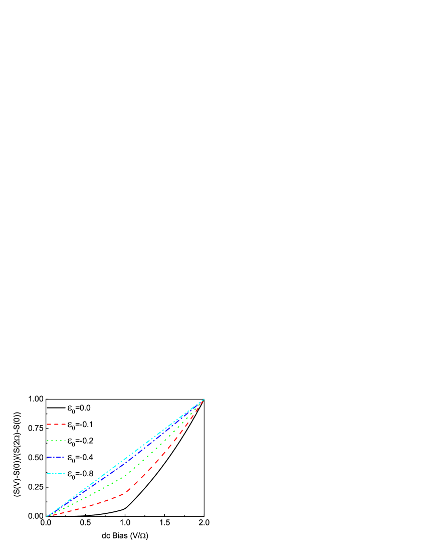
Figure 2: Noise of noninteracting quantum dot with ac gate field as a function of the applied dc bias for different values of energy level.

For a non-interacting quantum dot, analysis based on the scattering approach has shown that the photo-assisted noise as a function of the dc bias displays cusps at integer $\Omega/V$PRL72538 . The derivation of the noise then gives staircase behavior. Such singularities can be attributed to the change of the distribution of the transmitted charge by ac field. Here, we calculate the photon-assisted noise through a noninteracting quantum dot with ac gate by the Floquet-Green’s function method and noise formula Eq. (II.3). Identical numerical results are also obtained by the noise formula presented in Ref. PRL90210602 which is valid for ac transport in the absence of Coulomb interaction. In Fig. 2, we present the time-averaged noise power (in unit $\frac{e^{2}\Gamma_{0}}{h}$) as a function of dc bias voltage $V$ of ac gate modulated noninteracting dots for different dot energy levels. In the calculation, the temperature is fixed at $T=0.002$. The ac frequency is chosen as $\Omega=0.2$ and the ac strength is $V_{ac}=\Omega$. Since the magnitude of noise varies a lot with the energy level position, we have rescaled the $y$ axis to make the time-averaged noise $S(V)$ behavior at $V/\Omega=1$ more clearly. We can see from Fig. 2 that the appearance of cusp in the photon-assisted noise depends on the position of the energy level of the quantum dot. When $\epsilon_{d}=0$, i.e. the dot is in resonance, the noise shows an obvious cusp at $V=\Omega$. The cusp is ascribed to the non-adiabatic photon-assisted tunnelingPRL72538 . Since we have chosen a nonzero temperature, the sharpness of this cusp has been smoothed. When we lower the energy level and tune the dot out of resonance, the noise curves become smooth around $eV_{dc}=\hbar\Omega_{ac}$. These results indicate that the singularity of $dS/dV$ for noninteracting dot in the presence of ac gate modulation is most pronounce when the dot is situated at resonance. However, when the dot is far from resonance, the noise behaviors become smooth and it is hard for experiments to detect the noise singularity behavior.

We have shown that the non-interacting resonant dot can display noise singularity when the dot is modulated by ac gate. An intuitive analogous between the noninteracting resonant dot and the Kondo resonance, where both resonances can reach the conductance quanta ($2e^{2}/h$ with spin degeneracy), may lead to the naive conclusion that the noise of Kondo dot will show singularity in the presence of ac gate since there is Kondo resonance at Fermi energy. However, this statement is not correct, at least in the strongly correlated infinite-$U$ regime, as shown in our numerical results Fig. 3. In Fig. 3, we show the noise properties of the Kondo dot with different ac frequency as a function of the applied dc voltage. Since we are interested in the noise behavior at $V/\Omega=1$, the $x$ axis is rescaled by the ac frequency to have a better view at $V/\Omega=1$ (note different values of $\Omega$ in different curves). In Fig. 3, no singularity is observed at $V/\Omega=1$ for all the ac parameters. For lowest ac frequency ($\Omega=1\ T_{K}$), this is in agree with our previous results obtained by slave-boson mean-field approximationPRB77233307 . The noise at weak ac field is almost identical to the numerical results without ac field. It is interesting to see that both the slave-boson mean-field approximation and noncrossing approximation, which are valid in their respective parameter space, show that the noise of Kondo dot remains almost unaffected by the ac gate. The Kondo dot behaves as if the ac gate is effectively screened to induce singularity in the noise behavior. Comparing with the noninteracting resonance tunneling, the disappear of singularity behavior in noise of Kondo dot may be ascribed to the fact that the electrons through the Kondo resonance are not directly modulated by the ac field. Although the energy level of the quantum dot $\epsilon_{d}^{0}$ is periodically modulated by the ac gate, the Kondo peak is not directly driven by the ac field. For weak ac field where the ac frequency or ac strength are not in the order of the coupling strength or the energy level, the ac gate voltage is too small to drive the dot out of the Kondo regime. Strong correlation can still give rise to the sharp Kondo peak at Fermi energy. From the numerical results of LDOS, we can see that ac modulation of Kondo peak is much smaller than the applied ac gate which modulated the energy level of the dot. When the electrons are tunneling though the dot via the Kondo resonance, their transport behavior is not significantly modulated by the ac field. The influence of the time-periodicity of the Kondo peak to the electrons transport through the dot is negligibly small to show any singularities in the noise behavior. However, when the ac strength is strong enough to be comparable to $\epsilon_{d}^{0}$ or $\Gamma$, for example $\Omega=20\ T_{K}$ in Fig. 1 and 3, the quantum dot can sometimes be driven out of the Kondo regime by the ac field. The magnitude of the Kondo peak can then be significantly suppressed due to the strong ac field. As a consequence, the conductance declines drastically and deviates from the unitary limit. In these situations, the Kondo peak is then significantly suppressed and electron transmission probability becomes too small to show significant noise singularity.

Since the cusp of noise behavior can be smoothed by finite temperature, it is important to exclude the possibility that the smooth noise behavior shown in Fig. 3 is due to the finite temperature ($T=0.01<T_{K}$) in our numerical simulation. In Fig. 4, we plot the noise behavior as a function of dc bias voltage for the dot with different temperature. The ac frequency and ac strength is fixed at $\Omega=V_{ac}=1\ T_{K}$. The temperatures are chosen to be 0.01, 0.005 and 0.001, respectively. From Fig. 4, we can see that even for the lowest temperature $(T=0.001)$ which is much lower than $T_{K}$, no cusp is observed at $V/\Omega=1$ in the noise behavior. Together with the numerical results presented in Ref. PRB77233307, where no singularity is observed at zero temperature, the disappearance of cups in noise behavior can not be ascribed to the finite temperature. It is a generic feature of the strongly-correlated nature of Kondo peak.

Our numerical results together with those of Ref. PRB77233307 which are obtained with the help of the slave-boson technique have clearly shown that the strongly-correlated Kondo resonance can display different noise behavior as compared with the noninteracting dot. Usually, both the noninteracting resonant tunneling and Kondo resonance will lead to similar results in conductance measurement. Therefore, it is possible to make use of the distinct photon-assisted noise behavior to tell apart whether the resonant transport is via noninteracting resonance or strongly-correlated Kondo resonance. Such measurement has been in the reach of present technology. The recent experiment workPRL802437 ; PRL100026601 has shown the possibility to conduct the noise measurement of nanostructures with ac field. The ability to distinguish the origin of the resonant transport may be helpful to answer the controversy about origin of the 0.7 anomaly in quantum point contacts, where the zero bias anomaly is due to whether the formation of strongly correlated Kondo peakPRL89196802 or single-particle resonant peakPRB75045346 ; PRB79153303 is still under debating. We wish the experiment of the photon-assisted noise measurement can be used to reveal the underlying physics of 0.7 anomaly.

IV Conclusions

In conclusion, we have presented a Floquet-Green’s function formalism to investigate the noise properties of quantum dots in the ac-Kondo regime. The Coulomb correlation is taken into account by the infinite-$U$ NCA. In principle, the ac effect can be considered non-perturbatively via the infinite Floquet states. Our results show that the Kondo peak is robust against weak ac gate modulation. Significant suppression of the Kondo peak can be observed when the ac gate field becomes strong. The photon-assisted noise of Kondo dots as a function of dc voltage does not show singularities which are expected for noninteracting resonant quantum dot at integer $eV/\hbar\Omega$, where $V$ is the dc bias voltage and $\Omega$ is the ac frequency. These results suggest that we can tell resonant transport apart from the Kondo resonance by photon-assisted noise measurement, which can not be distinguished via the conductance measurement.

Appendix

In this appendix, we outline the derivation to reach the resolvent form of the Floquet-Green’s function. It resembles much to the resolvent form of the Green’s function at steady state. The starting point is the definition of Green’s function in time domain

$$(i\hbar\frac{\partial}{\partial t}-H(t))G(t,t^{\prime})=\delta(t-t^{\prime})$$ (57)

Make Fourier transform to the two side of Eq. [57]

$$\int e^{i\omega(t-t^{\prime})}dt^{\prime}(i\hbar\frac{\partial}{\partial t}-H(t))G(t,t^{\prime})=1$$ (58)

The Fourier transform of the Green’s function is defined as

$$G(t,t^{\prime})=\int\frac{d\omega^{\prime}}{2\pi}e^{-\omega^{\prime}(t-t^{\prime})}G(t,\omega^{\prime}).$$ (59)

Inserting Eq. (59) into (58), we have

$$\int e^{i\omega(t-t^{\prime})}dt^{\prime}(i\hbar\frac{\partial}{\partial t}-H(t))\int\frac{d\omega^{\prime}}{2\pi}e^{-\omega^{\prime}(t-t^{\prime})}G(t,\omega^{\prime})$$ (60)

$$= \int\int e^{i(\omega-\omega^{\prime})(t-t^{\prime})}(\hbar\omega^{\prime}+i\hbar\frac{\partial}{\partial t}-H(t))G(t,\omega^{\prime})dt^{\prime}\frac{d\omega^{\prime}}{2\pi}$$

$$= \int\delta(\omega-\omega^{\prime})d\omega^{\prime}(\hbar\omega^{\prime}-\mathcal{H}_{F}(t))G(t,\omega^{\prime})$$

$$= [\hbar\omega-\mathcal{H}_{F}(t)]G(t,\omega)=\bm{1}$$

where we have introduced the Floquet Hamiltonian $\mathcal{H}_{F}(t)=H(t)-i\hbar\frac{\partial}{\partial t}$.

Therefore, we arrive at the resolvent form of the Green’s function

$$G(t,\omega)=\frac{1}{\hbar\omega-\mathcal{H}_{F}(t)}$$ (61)

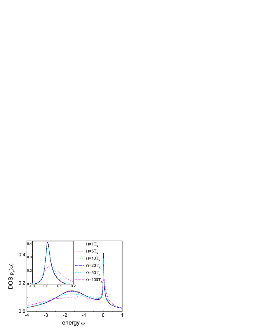
Figure 1: LDOS of Kondo quantum dots in the presence of ac gate modulation for different ac frequencies. The ac strength is fixed at $eV_{ac}/\hbar\Omega=1$.

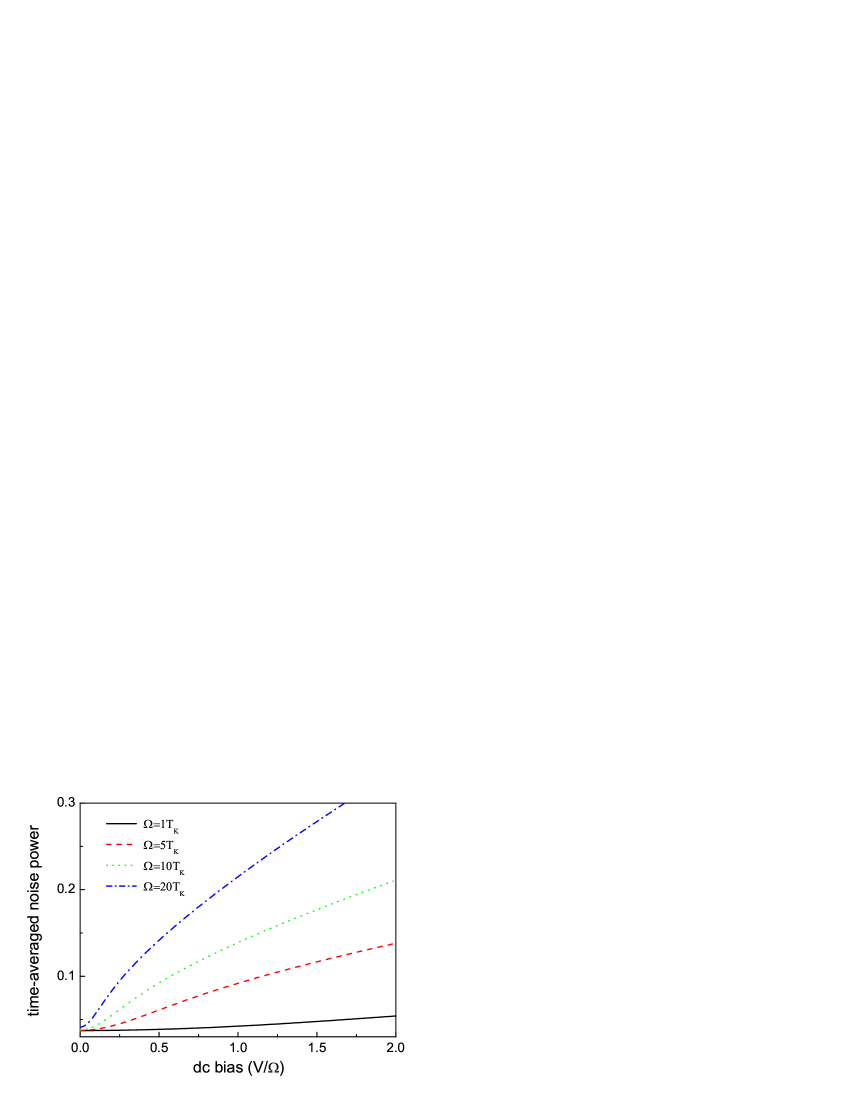
Figure 3: Noise of Kondo dot as a function of applied dc bias at fixed $eV_{ac}/\hbar\Omega=1$ and for four different values of frequency (in unit of the Kondo temperature). No singularities are observed at $eV_{dc}/\hbar\Omega=1$ for the different ac field parameters.

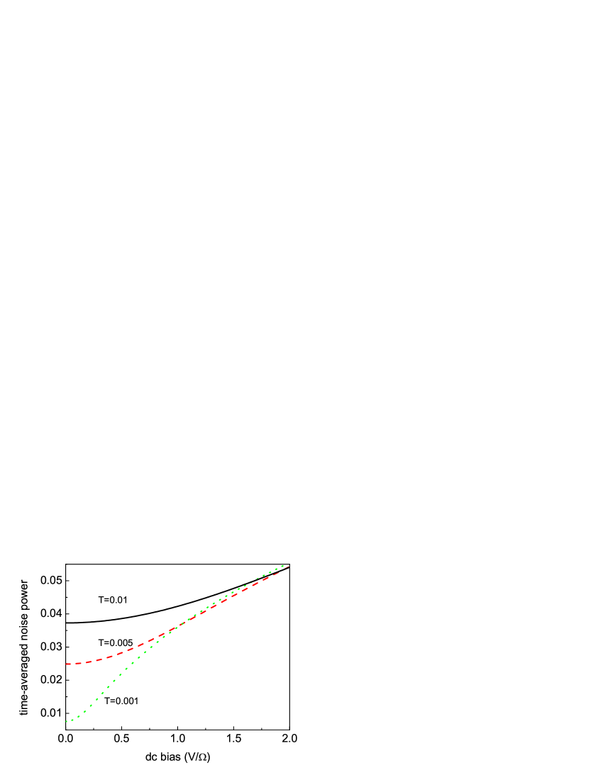
Figure 4: Noise of Kondo dot as a function of applied dc bias for different temperatures. The ac frequency and ac strength are fixed at $1\ T_{K}$.

References

- (1) A. C. Hewson, The Kondo Problem to Heavy Fermions (Cambridge University Press, Cambridge, 1993);
- (2) T. K. Ng and P. A. Lee, Phys. Rev. Lett. 61, 1768 (1988);
- (3) L. I. Glazman and M. E. Raikh, Pis’ma Zh. Éksp. Teor. Fiz. 47, 378 (1988) [JETP Lett. 47, 452 (1988)];
- (4) D. Goldhaber-Gordon, H. Shtrikman, D. Mahalu, D. Abusch-Magder, U. Meirav, and M. A. Kastner, Nature 391, 1569 (1998);
- (5) S. . Cronenwett, T. H. Oosterkamp, and L. P. Kouwenhoven, Sience 281, 540 (1998);
- (6) J. Nygard, D. H. Cobden, and P. E. Lindelof, Nature 408, 342 (2000);
- (7) J. Park, A. N. Pasupathy, J. I. Goldsmith, C. Chang, Y. Yaish, J. R. Petta, M. Rinkoski, J. P. Sethna, H. D. Abruna, P. L. McEuen, and D. C. Ralph, Nature 417, 722 (2002);
- (8) W. Liang, M. P. Shores, J. R. Long, and H. Park, Nature 417, 725 (2002);
- (9) V. Kashcheyevs, A. Aharony, and O. Entin-Wohlman, Phys. Rev. B 73, 125338 (2006);
- (10) N. E. Bickers, D. L. Cox, and J. W. Wilkins, Phys. Rev. B 36, 2036 (1987);
- (11) N. E. Bickers, Rev. Mod. Phys. 59, 845 (1987);
- (12) N. S. Wingreen, and Y. Meir, Phys. Rev. B 49, 11040 (1994);
- (13) for a review, see R. Bulla, T. A. Costi, and T. Pruschke, Rev. Mod. Phys. 80, 395 (2008);
- (14) Ya. M. Blantter and M. Büttiker, Phys. Rep. 336, 1 (2000);
- (15) Y. Meir and A. Golub, Phys. Rev. Lett. 88, 116802 (2002);
- (16) M. Sindel, W. Hofstetter, J. von Delft, and M. Kindermann, Phys, Rev. Lett., 94, 196602 (2005);
- (17) E. Sela, Y. Oreg, F. von Oppen, and J. Koch, Phys. Rev. Lett. 97, 086601 (2006);
- (18) A. Golub, Phys. Rev. B 75, 155313 (2007);
- (19) O. Zarchin, M. Zaffalon, M. Heiblum, D. Mahalu, and V. Umansky, Phys. Rev. B 77, 241303(R) (2008);
- (20) T. Delattre, C. Feuillet-Palma, L. G. Herrmann, P. Morfin, J.-M. Berroir, G. Fève, B. Plaçais, D. C. Glattli, M.-S. Choi, C. Mora and T. Kontos, Nature Physics 5, 208 (2009);
- (21) G. B. Lesovik, and L. S. Levitov, Phys. Rev. Lett. 72, 538 (1994);
- (22) R. J. Schoelkopf, A. A. Kozhevnikov, D. E. Prober, and M. J. Rooks, Phys. Rev. Lett. 80, 2437 (1998);
- (23) A. Lamacraft, Phys. Rev. Lett. 91, 036804 (2003);
- (24) M. Guigou, A. Popoff, T. Martin, and A. Crépieux, Phys. Rev. B 76, 045104 (2007);
- (25) M. H. Hettler and H. Schoeller, Phys. Rev. Lett. 74, 4907 (1995);
- (26) T. K. Ng, Phys. Rev. Lett. 76, 487 (1996);
- (27) G.-H. Ding and T. K. Ng, Phys. Rev. B 56, 15521(R) (1997);
- (28) P. Nordlander, M. Pustilnik, Y. Meir, N. S. Wingreen, and D. C. Langreth, Phys. Rev. Lett. 83, 808 (1999);
- (29) P. Nordlander, N. S. Wingreen, Y. Meir, and D. C. Langreth, Phys. Rev. B 61, 2146 (2000);
- (30) R. López, R. Aguado, G. Platero, and C. Tejedor, Phys. Rev. Lett. 81, 4688 (1998);
- (31) Y. Goldin, and Y. Avishai, Phys. Rev. Lett. 81, 5394 (1998);
- (32) Q. Chen and H. K. Zhao, Europhys. Lett. 82, 68004 (2008);
- (33) B. H. Wu, and J. C. Cao, Phys. Rev. B 77, 233307 (2008);
- (34) H. Shao, D. C. Langreth, and P. Nordlander, Phys. Rev. B 49, 13929 (1994);
- (35) R. Aguado, and D. C. Langreth, Phys. Rev. B 67, 245307 (2003);
- (36) J. Kroha, and P. Wölfle, J. Phys. Soc. Jpn. 74, 16 (2005);
- (37) J. Kroha, P. Wölfle, and T. A. Costi, Phys. Rev. Lett. 79, 261 (1997);
- (38) G. Platero and R. Aguado, Phys. Rep. 395, 1 (2004);
- (39) S. Kohler, J. Lehmann, and P. Hänggi, Phys. Rep. 406, 379 (2005);
- (40) A. Kaminski, Y. V. Nazarov, and L. I. Glazman, Phys. Rev. Lett. 83, 384 (1999);
- (41) H. Haug and A.-P. Jauho, Quantum Kinetics in Transport and Optics of Semiconductors (Springer-Verlag, Berlin, 1998).
- (42) J. H. Shirley, Phys. Rev. 138, B979, (1965).
- (43) M. Grifoni and P. Hänggi, Phys. Rep. 304, 229 (1998).
- (44) S. Camalet, J. Lehmann, S. Kohler, and P. Hänggi, Phys. Rev. Lett. 90, 210602 (2003);
- (45) L. E. F. Foa Torres, Phys. Rev. B 72, 245339 (2005);
- (46) L. Arrachea, Phys. Rev. B 72, 125349 (2005);
- (47) L. Arrachea, A. L. Yeyati, and A. Martin-Rodero, Phys. Rev. B 77, 165326 (2008);
- (48) B. H. Wu and J. C. Cao, J. Phys.:Condens. Matter 20, 085224 (2008);
- (49) A.-P. Jauho, N. S. Wingree, and Y. Meir, Phys. Rev. B 50, 5528 (1994);
- (50) J. Gabelli, and B. Reulet, Phys. Rev. Lett. 100, 026601 (2008);
- (51) Y. Meir, K. Hirose, and N. S. Wingreen, Phys. Rev. Lett. 89, 196802 (2002);
- (52) A. Lassl, P. Schlagheck, and K. Richter, Phys. Rev. B 75, 045346 (2007);
- (53) T.-M. Chen, A. C. Graham, M. Pepper, I. Farrer, and D. A. Ritchie, Phys. Rev. B 79, 153303 (2009);