Screened QED corrections in lithiumlike heavy ions in the presence of magnetic fields

Abstract

A rigorous evaluation of the complete gauge-invariant set of the screened one-loop QED corrections to the hyperfine structure and g factor in lithiumlike heavy ions is presented. The calculations are performed in both Feynman and Coulomb gauges for the virtual photon mediating the interelectronic interaction. As a result, the most accurate theoretical predictions for the specific difference between the hyperfine splitting values of H- and Li-like Bi ions as well as for the g factor of Li-like Pb ion are obtained.

Investigations of the hyperfine splitting and the g factor in highly charged ions give an access to a test of bound-state QED in strongest electromagnetic fields available at present for experimental study. To date, accurate measurements of the ground-state hyperfine structure and of the g factor were performed in H-like ²⁰⁹Bi, ¹⁶⁵Ho, ¹⁸⁵Re, ¹⁸⁷Re, ²⁰⁷Pb, ²⁰³Tl, and ²⁰⁵Tl Klaft et al. (1994); Crespo López-Urrutia et al. (1996, 1998); Seelig et al. (1998); Beiersdorfer et al. (2001) and in H-like ¹²C Häffner et al. (2000) and ¹⁶O Verdú et al. (2004), respectively. In particular, the 2002 CODATA value for the electron mass is derived mainly from the experimental and theoretical g factor values for hydrogenlike carbon and oxygen with an accuracy 4 times better than that of the 1998 CODATA value. An extension of such kind of experiments to highly charged Li-like ions presently being prepared Winters et al. (2007); Vogel et al. (2008) will provide the possibility to investigate a specific difference between the corresponding values of H- and Li-like ions, where the uncertainty due to the nuclear effects can be substantially reduced Shabaev et al. (2001); Glazov et al. (2004); Shabaev et al. (2006). Achievement of the required theoretical accuracy for the hyperfine structure and for the g factor in the case of Li-like ions is a very interesting and demanding challenge for theory.

At present, the theoretical accuracy of the specific difference of the hyperfine splitting values of H- and Li-like ions and of the g factor of Li-like heavy ions is mainly limited by uncertainties of the screened QED and higher-order interelectronic-interaction corrections. In the present Letter we focus on one of the most difficult correction, namely, the screened QED correction in the presence of a magnetic field perturbation. State-of-the-art evaluations of the screened QED correction were performed with local screening potentials Sapirstein and Cheng (2001); Glazov et al. (2006); Volotka et al. (2008). These calculations are based on the well-established technique developed for the evaluation of the one-loop QED corrections in the presence of an external potential Persson et al. (1996). However, the employment of a local screening potential does not allow one to take into account consistently all the contributing diagrams and to provide a reliable estimation of the uncertainty of the result. Therefore, a systematic description in the framework of QED requires the use of perturbation theory. This crucial step has been made now and in this Letter we report on our results of the rigorous evaluation of the complete gauge-invariant set of the screened one-loop QED corrections. As the most interesting application of these results towards tests of the magnetic sector of bound-state QED we present improved theoretical predictions for the specific difference between the ground-state hyperfine splitting values of H- and Li-like Bi ions and for the g factor of Li-like Pb ion.

The screened radiative correction in the presence of an external potential corresponds to the third-order perturbation theory terms. Nowadays, several approaches are used for derivation of the formal expressions from the first principles of QED: the two-time Green-function method Shabaev (2002), the covariant-evolution-operator method Lindgren et al. (2004), and the line profile approach O. Yu. Andreev et al. (2008). Here, we employ the two-time Green-function method. To simplify the derivation of formal expressions, we specify the formalism regarding the closed shell electrons as belonging to a redefined vacuum. It implies a modification of the $i0$-prescription in the electron propagator incorporating the closed-shell electrons. The corresponding shift of the Fermi-level does not affect the hyperfine structure and the g factor. In this way we have to consider all two-loop diagrams for the valence electron in the presence of magnetic perturbation, this is 27 nonequivalent diagrams. These diagrams merge the second-order interelectronic-interaction correction, the two-loop, and the screened one-loop radiative corrections. The generic types of the resulting screened self-energy diagrams are depicted in Fig. 1.

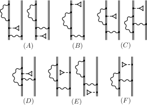
Figure 1: Feynman diagrams representing the screened self-energy correction in the presence of an external potential. The wavy line indicates the photon propagator and the double line indicates the electron propagators in the Coulomb field. The dashed line terminated with the triangle denotes the interaction with magnetic field.

The radiative correction to the hyperfine splitting $x_{\rm rad}$ can be written as the sum $x_{\rm rad}=x_{\rm QED}+x_{\rm SQED}$, where $x_{\rm QED}$ corresponds to the one-electron QED correction, and $x_{\rm SQED}$ stands for the screened radiative correction. The latter can be divided into self-energy (SE) and vacuum-polarization (VP) parts, $x_{\rm SQED}=x^{\rm SE}_{\rm SQED}+x^{\rm VP}_{\rm SQED}$. The screened SE correction can be distinguished according to so-called irreducible (irr) and reducible (red) parts. It appears as the sum of the following terms:

$$x^{\rm A,irr}_{\rm SQED}=2G_{a}\sum_{b}\sum_{P}(-1)^{P}\Biggl{\{}\sum_{n}^{\varepsilon_{n}\neq\varepsilon_{a}}\langle a|\Sigma(\varepsilon_{a})|n\rangle\hskip 28.45274pt$$

$$\times\frac{\langle nb|I(\Delta)|\xi_{Pa}Pb\rangle+\langle n|T_{0}|\zeta_{b|PaPb}\rangle}{\varepsilon_{a}-\varepsilon_{n}}+(a\leftrightarrow b)\Biggr{\}}\,,$$ (1)

$$x^{\rm B,irr}_{\rm SQED} = 2G_{a}\sum_{b}\sum_{P}(-1)^{P}\Bigl{\{}\langle\xi_{a}|\Sigma(\varepsilon_{a})|\zeta_{b|PaPb}\rangle$$ (2)

$$+ (a\leftrightarrow b)\Bigr{\}}\,,$$

$$x^{\rm C,irr}_{\rm SQED}=2G_{a}\sum_{b}\sum_{P}(-1)^{P}\frac{i}{2\pi}\int_{-\infty}^{\infty}{\rm d}\omega\sum_{n_{1},\,n_{2}}\hskip 28.45274pt$$

$$\times\Biggl{\{}\frac{\langle an_{1}|I(\omega)|n_{2}\xi_{Pa}\rangle\langle n_{2}b|I(\Delta)|n_{1}Pb\rangle}{(\varepsilon_{Pa}-\omega-u\varepsilon_{n_{1}})(\varepsilon_{a}-\omega-u\varepsilon_{n_{2}})}\hskip 39.83368pt$$

$$+\frac{\langle an_{1}|I(\omega)|n_{2}\zeta_{b|PaPb}\rangle\langle n_{2}|T_{0}|n_{1}\rangle}{(\varepsilon_{a}-\omega-u\varepsilon_{n_{1}})(\varepsilon_{a}-\omega-u\varepsilon_{n_{2}})}+(a\leftrightarrow b)\Biggr{\}}\,,$$ (3)

$$x^{\rm D,irr}_{\rm SQED} = 2G_{a}\sum_{b}\sum_{P}(-1)^{P}\frac{i}{2\pi}\int_{-\infty}^{\infty}{\rm d}\omega\sum_{n_{1},\,n_{2},\,n_{3}}\hskip 28.45274pt$$ (4)

$$\times \Biggl{\{}\frac{\langle an_{1}|I(\omega)|n_{3}Pa\rangle\langle n_{3}b|I(\Delta)|n_{2}Pb\rangle}{(\varepsilon_{Pa}-\omega-u\varepsilon_{n_{1}})(\varepsilon_{Pa}-\omega-u\varepsilon_{n_{2}})}$$

$$\times \frac{\langle n_{2}|T_{0}|n_{1}\rangle}{(\varepsilon_{a}-\omega-u\varepsilon_{n_{3}})}+(a\leftrightarrow b)\Biggr{\}}\,,$$

$$x^{\rm E,irr}_{\rm SQED}=2G_{a}\sum_{b}\sum_{P}(-1)^{P}\Biggl{\{}\sum_{n}^{\varepsilon_{n}\neq\varepsilon_{a}}\langle a|\Sigma(\varepsilon_{a})|n\rangle\hskip 28.45274pt$$

$$\times\frac{\langle n\xi_{b}|I(\Delta)|PaPb\rangle+\langle nb|I(\Delta)|Pa\xi_{Pb}\rangle}{\varepsilon_{a}-\varepsilon_{n}}+(a\leftrightarrow b)\Biggr{\}}\,,$$ (5)

$$x^{\rm F,irr}_{\rm SQED}=2G_{a}\sum_{b}\sum_{P}(-1)^{P}\frac{i}{2\pi}\int_{-\infty}^{\infty}{\rm d}\omega\sum_{n_{1},\,n_{2}}\hskip 34.14322pt$$

$$\times\Biggl{\{}\frac{\langle an_{1}|I(\omega)|n_{2}Pa\rangle\langle n_{2}\xi_{b}|I(\Delta)|n_{1}Pb\rangle}{(\varepsilon_{Pa}-\omega-u\varepsilon_{n_{1}})(\varepsilon_{a}-\omega-u\varepsilon_{n_{2}})}+(a\leftrightarrow b)\Biggr{\}}\,,$$ (6)

$$x^{\rm G,red}_{\rm SQED}=2\,G_{a}\sum_{b}\sum_{P}(-1)^{P}\Biggl{\{}\langle a|\Sigma(\varepsilon_{a})\Biggl{[}|\zeta^{\prime}_{b|PaPb}\rangle\hskip 17.07182pt$$

$$\times\langle a|T_{0}|a\rangle+|\xi^{\prime}_{a}\rangle\langle ab|I(\Delta)|PaPb\rangle+|a\rangle\langle\zeta^{\prime}_{b|PaPb}|T_{0}|a\rangle$$

$$+|a\rangle\Bigl{(}\langle a|T_{0}|a\rangle-\langle b|T_{0}|b\rangle\Bigr{)}\frac{\langle ab|I^{\prime\prime}(\Delta)|PaPb\rangle}{2}\delta_{bPa}\hskip 18.49411pt$$

$$+|\xi_{a}\rangle\langle ab|I^{\prime}(\Delta)|PaPb\rangle+|a\rangle\langle ab|I^{\prime}(\Delta)|\xi_{Pa}Pb\rangle\hskip 31.2982pt$$

$$-\sum_{n}^{\varepsilon_{n}\neq\varepsilon_{a}}\frac{\langle nb|I^{\prime}(\Delta)|PaPb\rangle\langle b|T_{0}|b\rangle}{\varepsilon_{a}-\varepsilon_{n}}\,|n\rangle\Biggr{]}+(a\leftrightarrow b)\Biggr{\}}\,,\hskip 5.69046pt$$ (7)

$$x^{\rm H,red}_{\rm SQED}=G_{a}\sum_{b}\sum_{P}(-1)^{P}\Biggl{\{}\frac{i}{2\pi}\int_{-\infty}^{\infty}{\rm d}\omega\sum_{n_{1},\,n_{2}}\hskip 31.2982pt$$

$$\times\Biggl{[}\frac{\langle an_{1}|I(\omega)|n_{2}a\rangle\langle n_{2}|T_{0}|n_{1}\rangle\langle ab|I^{\prime}(\Delta)|PaPb\rangle}{(\varepsilon_{a}-\omega-u\varepsilon_{n_{1}})(\varepsilon_{a}-\omega-u\varepsilon_{n_{2}})}\hskip 29.87547pt$$

$$+2\frac{\langle an_{1}|I(\omega)|n_{2}Pa\rangle\langle n_{2}b|I^{\prime}(\Delta)|n_{1}Pb\rangle\langle a|T_{0}|a\rangle}{(\varepsilon_{Pa}-\omega-u\varepsilon_{n_{1}})(\varepsilon_{a}-\omega-u\varepsilon_{n_{2}})}\Biggr{]}\hskip 24.18501pt$$

$$+2\langle a|\Sigma^{\prime}(\varepsilon_{a})\Biggl{[}|\xi_{a}\rangle\langle ab|I(\Delta)|PaPb\rangle+|\zeta_{b|PaPb}\rangle\langle a|T_{0}|a\rangle$$

$$+|a\rangle\Bigl{(}\langle a|T_{0}|a\rangle-\frac{\langle b|T_{0}|b\rangle}{2}\Bigr{)}\langle ab|I^{\prime}(\Delta)|PaPb\rangle\hskip 42.67912pt$$

$$+|a\rangle\Bigl{(}\langle\zeta_{b|PaPb}|T_{0}|a\rangle+\langle\zeta_{a|PbPa}|T_{0}|b\rangle\Bigr{)}\Biggr{]}+(a\leftrightarrow b)\Biggr{\}}\,,$$ (8)

$$x^{\rm I,red}_{\rm SQED}=-G_{a}\sum_{b}\sum_{P}(-1)^{P}\Biggl{\{}\frac{i}{2\pi}\int_{-\infty}^{\infty}{\rm d}\omega\sum_{n_{1},\,n_{2}}\hskip 31.2982pt$$

$$\times\Biggl{[}\frac{\langle an_{1}|I(\omega)|n_{2}a\rangle\langle ab|I(\Delta)|PaPb\rangle}{(\varepsilon_{a}-\omega-u\varepsilon_{n_{1}})(\varepsilon_{a}-\omega-u\varepsilon_{n_{2}})}\Biggl{(}\frac{\langle n_{2}|T_{0}|n_{1}\rangle}{\varepsilon_{a}-\omega-u\varepsilon_{n_{1}}}\hskip 14.22636pt$$

$$+\frac{\langle n_{2}|T_{0}|n_{1}\rangle}{\varepsilon_{a}-\omega-u\varepsilon_{n_{2}}}\Biggr{)}+\frac{\langle an_{1}|I(\omega)|n_{2}Pa\rangle\langle n_{2}b|I(\Delta)|n_{1}Pb\rangle}{(\varepsilon_{Pa}-\omega-u\varepsilon_{n_{1}})(\varepsilon_{a}-\omega-u\varepsilon_{n_{2}})}$$

$$\times\Biggl{(}\frac{\langle Pa|T_{0}|Pa\rangle}{\varepsilon_{Pa}-\omega-u\varepsilon_{n_{1}}}+\frac{\langle a|T_{0}|a\rangle}{\varepsilon_{a}-\omega-u\varepsilon_{n_{2}}}\Biggr{)}\Biggl{]}\hskip 64.01869pt$$

$$-\langle a|\Sigma^{\prime\prime}(\varepsilon_{a})|a\rangle\langle a|T_{0}|a\rangle\langle ab|I(\Delta)|PaPb\rangle+(a\leftrightarrow b)\Biggr{\}}\,.\hskip 14.22636pt$$ (9)

Here, $a$ and $b$ denotes the valence and core electron states, respectively, the sum over $b$ runs over all closed-shell states, $P$ is the permutation operator, giving rise to the sign $(-1)^{P}$ of the permutation, and the notation $(a\leftrightarrow b)$ stands for the contribution with interchanged labels $a$ and $b$. The SE operator $\Sigma(\varepsilon)$, the interelectronic-interaction operator $I(\omega)$, and their derivatives (indicated by primes) are defined similar as in Ref. Shabaev (2002), $u=1-i0$ preserves the proper treatment of poles of the electron propagators. The energy difference $\Delta$ is defined as $\Delta=\varepsilon_{a}-\varepsilon_{Pa}$ and, accordingly, $\Delta=\varepsilon_{b}-\varepsilon_{Pb}$ in terms $(a\leftrightarrow b)$. $T_{0}$ is the electronic part of the hyperfine-interaction operator and $G_{a}$ is the multiplicative factor depending on the quantum numbers of the valence electron (see for details Ref. Volotka et al. (2008)). The wavefunctions $|\xi\rangle$, $|\zeta\rangle$, and $|\xi^{\prime}\rangle$, $|\zeta^{\prime}\rangle$ are defined as follows

$$|\xi_{a}\rangle=\sum_{n}^{\varepsilon_{n}\neq\varepsilon_{a}}\frac{|n\rangle\langle n|T_{0}|a\rangle}{\varepsilon_{a}-\varepsilon_{n}}\,,$$ (10)

$$|\zeta_{b|PaPb}\rangle=\sum_{n}^{\varepsilon_{n}\neq\varepsilon_{a}}\frac{|n\rangle\langle nb|I(\Delta)|PaPb\rangle}{\varepsilon_{a}-\varepsilon_{n}}\,,$$ (11)

and $|\xi^{\prime}_{a}\rangle=\frac{\partial}{\partial\varepsilon_{a}}|\xi_{a}\rangle$, $|\zeta^{\prime}_{b|PaPb}\rangle=\frac{\partial}{\partial\varepsilon_{a}}|\zeta_{b|PaPb}\rangle$.

The expressions compiled in Eqs. (Screened QED corrections in lithiumlike heavy ions in the presence of magnetic fields)-(Screened QED corrections in lithiumlike heavy ions in the presence of magnetic fields), and (Screened QED corrections in lithiumlike heavy ions in the presence of magnetic fields)-(Screened QED corrections in lithiumlike heavy ions in the presence of magnetic fields) contain ultraviolet divergences. We separate out the divergent zero- and one-potential terms in Eqs. (Screened QED corrections in lithiumlike heavy ions in the presence of magnetic fields), (2), (Screened QED corrections in lithiumlike heavy ions in the presence of magnetic fields), (Screened QED corrections in lithiumlike heavy ions in the presence of magnetic fields) and zero-potential terms in Eqs. (Screened QED corrections in lithiumlike heavy ions in the presence of magnetic fields), (Screened QED corrections in lithiumlike heavy ions in the presence of magnetic fields), (Screened QED corrections in lithiumlike heavy ions in the presence of magnetic fields) and evaluate these terms in the momentum space, where the divergences can be removed analytically (see, e.g., Ref. Yerokhin and Shabaev (1999)). The remaining many-potential terms are ultraviolet finite and calculated in coordinate space. The infrared divergences which occur in the terms of the Eqs. (Screened QED corrections in lithiumlike heavy ions in the presence of magnetic fields), (4), (Screened QED corrections in lithiumlike heavy ions in the presence of magnetic fields), (Screened QED corrections in lithiumlike heavy ions in the presence of magnetic fields), (Screened QED corrections in lithiumlike heavy ions in the presence of magnetic fields) are regularized by introducing a nonzero photon mass and canceled analytically.

The numerical evaluation is based on employing the dual-kinetic-balance finite basis set method Shabaev et al. (2004) with basis functions constructed from B-splines Sapirstein and Johnson (1996). The Fermi model for the nuclear charge density and the sphere model for the magnetic moment distribution have been employed. In what follows we present our result for the case of Li-like Bi utilizing the corresponding values for the nuclear properties: $\langle r^{2}\rangle^{1/2}=5.5211$ fm Angeli (2004), $I^{\pi}=9/2-$, and $\mu=4.1106(2)\mu_{N}$ Stone (2005). The calculations have been performed in Feynman and Coulomb gauges for the photon propagator describing the electron-electron interaction, thus providing an accurate check of the numerical procedure. The obtained results for the screened SE correction for the hyperfine splitting of the Li-like Bi are presented in Table 1 in both gauges, respectively.

Table 1: Individual contributions to the screened SE correction $x^{\rm SE}_{\rm SQED}$ for the ground-state hyperfine structure of the Li-like ²⁰⁹Bi⁸⁰⁺.

Contr.	Feynman	Coulomb	Contr.	Feynman	Coulomb
A, irr	0.001544	0.001555	F, irr	$-$0.000174	$-$0.000172
B, irr	$-$0.000380	$-$0.000398	G, red	$-$0.001298	$-$0.001307
C, irr	0.001928	0.001952	H, red	0.000331	0.000331
D, irr	$-$0.000936	$-$0.000945	I, red	0.000066	0.000066
E, irr	0.000028	0.000028
			Total	0.001109	0.001109

Finally, we have calculated the screened SE correction within local screening potentials: Kohn-Sham $0.0012$ and core-Hartree $0.0013$. The results are in reasonable agreement with the rigorous evaluation $x^{\rm SE}_{\rm SQED}=0.00111$.

We have also calculated the screened VP correction in the presence of a magnetic field employing the Uehling approximation for the VP loop. The results have been checked utilizing the Feynman and Coulomb gauges for the photon propagator mediating the interelectronic interaction. The electric-loop part of the screened Wichmann-Kroll (WK) contribution has been calculated by means of the approximate formulas for the WK potential from Ref. Fainshtein et al. (1990). As concerns the screened WK magnetic-loop part we have employed the hydrogenic $2s$ value from Ref. Artemyev et al. (2001), assuming that it enters with the same screening ratio as the Uehling terms. Accordingly, our value for the screened VP correction is $x^{\rm VP}_{\rm SQED}=-0.00054(2)$. Finally, the total value for the screened QED correction to the ground-state hyperfine structure in Li-like Bi results as $x_{\rm SQED}=0.00057(2)$.

Probing the influence of QED effects on the hyperfine splitting of highly charged ions is impeded by the uncertainty of the nuclear magnetization distribution correction [the Bohr-Weisskopf (BW) effect]. In this context, it was proposed to consider a specific difference of the ground state hyperfine splitting in H-like and Li-like ions Shabaev et al. (2001): $\Delta^{\prime}E=\Delta E^{(2s)}-\xi\Delta E^{(1s)}$, where $\Delta E^{(1s)}$ and $\Delta E^{(2s)}$ are the hyperfine splittings of H- and Li-like ions, respectively, the parameter $\xi$ is chosen to cancel the BW correction. In this specific difference the nuclear corrections almost vanish completely. We have recalculated the energy shift $\Delta^{\prime}E$ employing the most accurate result obtained for the screened QED correction. The interelectronic-interaction corrections have been evaluated to first-order in $1/Z$ within the QED perturbation theory and to higher-orders within the large-scale configuration-interaction Dirac-Fock-Sturm method. Extracting numerically the contribution of the BW effect in different terms we found that the cancellation appears with $\xi$ chosen to be $\xi=0.16886$ for the case of Bi. In Table 2 we present obtained result for the specific difference between the hyperfine structure values of H- and Li-like Bi ions. The Dirac value incorporates also the finite nuclear size correction.

Table 2: Individual contributions to the specific difference $\Delta^{\prime}E$ for ²⁰⁹Bi in meV.

	$\Delta E^{(2s)}$	$\xi\Delta E^{(1s)}$	$\Delta^{\prime}E$
Dirac value	844.829(4)	876.638	$-$31.809(4)
Interel. inter.,$\sim 1/Z$	$-$29.995(4)		$-$29.995(4)
Interel. inter.,$\sim 1/Z^{2}$ and h.o.	0.25(4)		0.25(4)
QED	$-$5.052(4)	$-$5.088	0.036(4)
Screened QED	0.194(6)		0.194(6)
Total			$-$61.32(4)

The nuclear-polarization correction to the $1s$ hyperfine splitting calculated in Ref. Nefiodov et al. (2003) yields $\xi\Delta E^{(1s)}_{\rm NP}=0.009$ meV. However, since all nuclear corrections have the similar scaling dependence upon the principal quantum numbers, we expect the strong cancellation between $1s$ and $2s$ nuclear-polarization corrections in the specific difference. The same is valid for the second-order one-electron QED contributions. Comparing with the results for the specific difference $\Delta^{\prime}E$ presented in Ref. Shabaev et al. (2001) we have increased the accuracy for the screened QED part and performed more elaborate calculations for the higher-order interelectronic-interaction correction. Further rigorous evaluation of the higher-order electron-electron interaction corrections will provide a test of bound-state QED at strongest electric and magnetic fields.

Similar calculations have been performed for the g factor of Li-like heavy ions. Here, we present our results for the case of ²⁰⁸Pb⁷⁹⁺ with the following value for the nuclear charge radius $\langle r^{2}\rangle^{1/2}=5.5010$ fm Angeli (2004). The rigorous evaluation of the screened SE correction gives $\Delta{\rm g}^{\rm SE}_{\rm SQED}=-3.1(1)\times 10^{-6}$. The previous value obtained with local screening potentials was $-3.5(1.2)\times 10^{-6}$ Glazov et al. (2006). Thus, the uncertainty of the screened SE correction has been reduced by an order of magnitude. The screened VP contribution has been calculated within the Uehling approximation. As to the WK part, we have employed the approximate formulas for the electric-loop potential Fainshtein et al. (1990), while the magnetic-loop value has been taken from Ref. Lee et al. (2005), assuming the same screening ratio as for the Uehling term. Accordingly, we have obtained $\Delta{\rm g}^{\rm VP}_{\rm SQED}=1.5\times 10^{-6}$. In Table 3 we have updated the value for the g factor of Li-like ²⁰⁸Pb⁷⁹⁺ previously reported in Ref. Glazov et al. (2006) employing the result obtained for the screened QED correction.

Table 3: Individual contributions to the ground-state g factor of Li-like ²⁰⁸Pb⁷⁹⁺.

Dirac value (point nucleus)	1.932 002 904
Finite nuclear size	0.000 078 58(13)
Interel. inter.	0.002 140 7(27)
QED, $\sim\alpha$	0.002 411 7(1)
QED, $\sim\alpha^{2}$	$-$ 0.000 003 6(5)
Screened QED	$-$ 0.000 001 6(1)
Nuclear recoil	0.000 000 25(35)
Nuclear polarization	$-$ 0.000 000 04(2)
Total	1.936 628 9(28)

Further extensions of these calculations to the g factor of B-like heavy ions may serve for an independent determination of the fine structure constant from QED at strong fields Shabaev et al. (2006).

In summary, we have rigorously calculated the screened QED correction to the hyperfine splitting and g factor of heavy Li-like ions. We have increased the theoretical accuracy for the specific difference between the hyperfine splitting values of H- and Li-like bismuth as well as for the g factor of Li-like lead. The rigorous calculation of the higher-order interelectronic-interaction correction will be the next step towards the unprecedented accuracy for the stringent test of the bound-state QED in the presence of magnetic fields.

The authors acknowledge financial support from DFG, GSI, RFBR (Grant No. 07-02-00126a), and Ministry of Education and Science of Russian Federation (Program for Development of Scientific Potential of High School, Grant No. 2.1.1/1136). The work of D.A.G. was also supported by the grant of President of Russian Federation (Grant No. MK-3957.2008.2) and by the FAIR - Russia Research Center.

References

- Klaft et al. (1994) I. Klaft et al., Phys. Rev. Lett. 73, 2425 (1994).
- Crespo López-Urrutia et al. (1996) J. R. Crespo López-Urrutia et al., Phys. Rev. Lett. 77, 826 (1996).
- Crespo López-Urrutia et al. (1998) J. R. Crespo López-Urrutia et al., Phys. Rev. A 57, 879 (1998).
- Seelig et al. (1998) P. Seelig et al., Phys. Rev. Lett. 81, 4824 (1998).
- Beiersdorfer et al. (2001) P. Beiersdorfer et al., Phys. Rev. A 64, 032506 (2001).
- Häffner et al. (2000) H. Häffner et al., Phys. Rev. Lett. 85, 5308 (2000).
- Verdú et al. (2004) J. Verdú et al., Phys. Rev. Lett. 92, 093002 (2004).
- Winters et al. (2007) D. F. A. Winters et al., Can. J. Phys. 85, 403 (2007).
- Vogel et al. (2008) M. Vogel et al., Eur. Phys. J. Special Topics 163, 113 (2008).
- Shabaev et al. (2001) V. M. Shabaev et al., Phys. Rev. Lett. 86, 3959 (2001).
- Glazov et al. (2004) D. A. Glazov et al., Phys. Rev. A 70, 062104 (2004).
- Shabaev et al. (2006) V. M. Shabaev et al., Phys. Rev. Lett. 96, 253002 (2006).
- Sapirstein and Cheng (2001) J. Sapirstein and K. T. Cheng, Phys. Rev. A 63, 032506 (2001).
- Glazov et al. (2006) D. A. Glazov et al., Phys. Lett. A 357, 330 (2006).
- Volotka et al. (2008) A. V. Volotka et al., Phys. Rev. A 78, 062507 (2008).
- Persson et al. (1996) H. Persson et al., Phys. Rev. Lett. 76, 1433 (1996); S. A. Blundell, K. T. Cheng, and J. Sapirstein, Phys. Rev. Lett. 78, 4914 (1997); V. M. Shabaev et al., Phys. Rev. A 56, 252 (1997); V. A. Yerokhin and V. M. Shabaev, Phys. Rev. A 64, 012506 (2001).
- Shabaev (2002) V. M. Shabaev, Phys. Rep. 356, 119 (2002).
- Lindgren et al. (2004) I. Lindgren, S. Salomonson, and B. Åsén, Phys. Rep. 389, 161 (2004).
- O. Yu. Andreev et al. (2008) O. Yu. Andreev et al., Phys. Rep. 455, 135 (2008).
- Yerokhin and Shabaev (1999) V. A. Yerokhin and V. M. Shabaev, Phys. Rev. A 60, 800 (1999).
- Shabaev et al. (2004) V. M. Shabaev et al., Phys. Rev. Lett. 93, 130405 (2004).
- Sapirstein and Johnson (1996) J. Sapirstein and W. R. Johnson, J. Phys. B 29, 5213 (1996).
- Angeli (2004) I. Angeli, At. Data Nucl. Data Tables 87, 185 (2004).
- Stone (2005) N. J. Stone, At. Data Nucl. Data Tables 90, 75 (2005).
- Fainshtein et al. (1990) A. G. Fainshtein, N. L. Manakov, and A. A. Nekipelov, J. Phys. B 23, 559 (1990).
- Artemyev et al. (2001) A. N. Artemyev et al., Phys. Rev. A 63, 062504 (2001).
- Nefiodov et al. (2003) A. V. Nefiodov, G. Plunien, and G. Soff, Phys. Lett. B 552, 35 (2003).
- Lee et al. (2005) R. N. Lee et al., Phys. Rev. A 71, 052501 (2005).