Signature of electronic excitations in the Raman spectrum of graphene.

Abstract

Inelastic light scattering from Dirac-type electrons in graphene is shown to be dominated by the generation of the inter-band electronic modes which are odd in terms of time-inversion symmetry and belong to the irreducible representation A₂ of the point group C_6v of the honeycomb crystal. At high magnetic fields, these electron-hole excitations appear as peculiar $n^{-}\rightarrow n^{+}$ inter-Landau-level modes with energies $\omega_{n}=2\sqrt{2n}\,\hbar v/\lambda_{B}$ and characteristically crossed polarisation of in/out photons.

Inelastic (Raman) scattering of light is a powerful tool to study excitations in solids Book-R . Recently, Raman spectroscopy has been used to study phonons in graphene Ferrari , where it has become the method of choice for determining the number of atomic layers in graphitic flakes Ferrari ; Graf ; CastroNeto1 ; Jiang ; Potemski1 ; Berciaud ; BalandinCalizo . In particular, single- and multiple-phonon-emission lines in the Raman spectrum of graphene and the influence of the electron-phonon coupling on the phonon spectrum have been investigated in great detail GeimNovoselov ; CastroNeto2 ; Basko1 ; Ando ; Kechedzhi ; Pinczuk1 ; Pinczuk2 ; FerrariBasko . However, no experimental observation or comprehensive theoretical analysis has been reported on the Raman spectroscopy of electronic excitations in graphene, despite extensive studies of optical absorption in this material Potemski2 ; Kim ; Kuzmenko ; Basov ; AbergelFalko ; Geim ; AbergelRussellFalko .

In this Letter, we present a theory of inelastic light scattering in the visible range of photon energies accompanied by electronic excitations in graphene. We classify the relevant modes according to their symmetry and predict peculiar selection rules for the Raman-active excitations of electrons between Landau levels in graphene at quantizing magnetic fields. Graphene is a gapless semiconductor Wallace ; RMPgraphene , with an almost linear Dirac-type spectrum, $\varepsilon=\alpha vp$ in the conduction ($\alpha=+$) and valence ($\alpha=-$) band, which touch each other in the corners of the hexagonal Brillouin zone, usually called valleys. The band structure of graphene is prescribed by the hexagonal symmetry C_6v of its honeycomb lattice, and it is natural to relate Raman-active modes to the irreducible representations of the point group C_6v. We argue that the dominant electronic modes generated by inelastic scattering of photons with energy $\Omega$ less than the bandwidth of graphene are superpositions of the interband electron-hole pairs which have symmetry of the representation A₂ of the group C_6v and are odd with respect to the inversion of time. Their excitation process consists of two steps: the absorption (emission) of a photon with energy $\Omega$ ($\tilde{\Omega}=\Omega-\omega$) transfering an electron from an occupied state in the valence band into a virtual state in the conduction band, followed by emission (absorption) of the second photon with energy $\tilde{\Omega}$ ($\Omega$). Its amplitude is determined by the sum of partial amplitudes distinguished by the order of absorption and emission of photons, and by which carrier in the intermediate state (an electron above the Fermi level or hole below it) undergoes the second optical transition. The dominance of such process over the process involving the contact interaction Platzmann-Wolff ; Chinese of an electron with two photons is a peculiarity of the Dirac-type electrons in graphene. Filling the conduction band or depleting the valence band, up to the Fermi level $\alpha\mu$, forbids the excitation of inter-band electron-hole pairs with energies $\omega<2\mu$ leading to the linear Raman spectrum with a $2\mu$ threshold [dashed line in Fig. 1]. The quantization of the electronic spectrum into Landau levels McClure (LL) $\varepsilon[n^{\alpha}]=\alpha\sqrt{2n}\,\hbar v/\lambda_{B}$ in a strong magnetic field ($\lambda_{B}=\sqrt{\hbar c/eB}$ is the magnetic length, $n=0,1,2,...$) makes Raman spectrum discrete at low energies $\omega_{n}=2\sqrt{2n}\,\hbar v/\lambda_{B}$, with peculiar for the Dirac-type electrons selection rules, $n^{-}\rightarrow n^{+}$ of the dominant Raman-active transitions [solid line in Fig. 1].

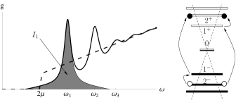
Figure 1: Spectral density $g(\omega)$ of light inelastically scatterred from electronic excitations in graphene at quantising magnetic fields (solid line) and at $B=0$ (dashed line). Here $\omega\ll\Omega$ is the Raman shift. Sketch illustrates intermediate and final states of the dominant Raman process.

The following theory is based upon the tight-binding model of electron states in graphene expanded into the Dirac-type Hamiltonian Dresselhaus ,

$$\mathcal{H}=v\boldsymbol{\Sigma}\cdot\mathbf{P}-\frac{v^{2}}{6\gamma_{0}}\Lambda^{z}\Sigma^{x}(\boldsymbol{\Sigma}\mathbf{P})\Sigma^{x}(\boldsymbol{\Sigma}\mathbf{P})\Sigma^{x}.$$ (1)

The latter describes electrons in the conduction and valence bands around the Brillouin zone (BZ) corners $K$ and $K^{\prime}$. We use notations McCann such that $\boldsymbol{\Sigma}=(\Pi_{KK^{\prime}}^{z}\otimes\sigma_{AB}^{x},\Pi_{KK^{\prime}}^{z}\otimes\sigma_{AB}^{y})$, $\Sigma^{z}=$ $\hat{1}_{KK^{\prime}}\otimes\sigma_{AB}^{z}$ and $\Lambda^{z}=\Pi_{KK^{\prime}}^{z}\otimes\hat{1}_{AB}$, where $\sigma_{AB}^{x/y/z}$ and $\Pi_{KK^{\prime}}^{x/y/z}$ are Pauli matrices acting on $A$-$B$ (sublattice) and $K$-$K^{\prime}$ (valley) indices of the four-component wave function $\{\psi_{K},\psi_{K^{\prime}}\}$, where $\psi_{K}=[\varphi_{A},\varphi_{B}]$ and $\psi_{K^{\prime}}=[\varphi_{B},\varphi_{A}]$. While 4-spinors $\{\psi_{K},\psi_{K^{\prime}}\}$ realise 4D irreducible representation of the full symmetry group of the crystal, the valley-diagonal operators $\Sigma^{i}$ and $\Lambda^{z}\Sigma^{i}$ can be combined into irreducible representations KechedzhiEPJ ; Basko1 of the group C_6v, Table 1, and $\Lambda^{z}$ is used to describe valley-asymmetry of Dirac electrons. The first term in $\mathcal{H}$ determines the linear spectrum $\alpha vp$ with $v\approx 10^{8}$cm/s  and $\mathbf{p}$ being the in-plane momentum counted from the BZ corner. The second term takes into account weak trigonal warping [hopping parameter $\gamma_{0}\approx 3$eV determines the bandwidth, $\sim 6\gamma_{0}$], which has an inverted shape in the opposite corners of the BZ Dresselhaus . The vector potential of light $\mathbf{A}=\sum_{\mathbf{l},\mathbf{q},q_{z}}\frac{\hbar c}{\sqrt{2\Omega}}\left(\mathbf{l}e^{i(\mathbf{q}\mathbf{r}-\Omega t)/\hbar}b_{\mathbf{q},q_{z},\mathbf{l}}+h.c.\right)$ is included in $\mathbf{P}=\mathbf{p}-\frac{e}{c}\mathbf{A}$, where $b_{\mathbf{q},q_{z},\mathbf{l}}$ annihilates a photon characterised by the polarisation [$\mathbf{l}$ for incident and $\mathbf{\tilde{l}}$ for scattered light], in-plane momentum $\mathbf{q}$, energy $\Omega$, and $q_{z}=\sqrt{\Omega^{2}/c^{2}-\mathbf{q}^{2}}$.

C6v rep.	A1	B1	A2	B2	E1	E2
matrix	$1$	$\Lambda^{z}$	$\Sigma^{z}$	$\Lambda^{z}\Sigma^{z}$	$\boldsymbol{\Sigma}$	$\Lambda^{z}\boldsymbol{e}_{z}\times\boldsymbol{\Sigma}$
$t\rightarrow-t$	$+$	$-$	$-$	$+$	$-$	$+$

Table 1: C_6v irreducible representations by the valley-diagonal operators $\Sigma^{i}$ and $\Lambda^{z}\Sigma^{i}$.

The amplitude $R=R_{D}+R_{w}+\mathcal{T}\widetilde{V}$ of the Raman process with the excitation of an electron-hole (e-h) pair in the final state corresponds to the Feynman diagrams shown in Fig. 2. Here, we call an ‘electron’ an excited quasiparticle above the Fermi level $\alpha\mu$, and a ‘hole’ an empty state at $\varepsilon<\alpha\mu$. The building blocks of the diagrams include Green’s functions for the electrons and the electron-photon interaction vertices:

$$= G_{\varepsilon,\mathbf{p}}^{R/A}=\frac{1}{2}\sum_{\alpha=\pm}\frac{1+\alpha\boldsymbol{\Sigma}\cdot\mathbf{n_{p}}}{\varepsilon-\alpha vp\pm i0},\qquad\mathbf{n_{p}=}\frac{\mathbf{p}}{p},$$

$$= \frac{ev\hbar}{\sqrt{2|\Omega|}}\boldsymbol{\Sigma}\cdot\mathbf{l},\qquad\raisebox{-12.0pt}{\begin{picture}(28.0,28.0)(-14.0,-14.0)\put(-8.0,-12.0){\oval(8.0,8.0)[tl]} \put(-8.0,-4.0){\oval(8.0,8.0)[br]} \put(0.0,-4.0){\oval(8.0,8.0)[tl]} \put(-4.0,-5.0){\vector(-1,-1){4.0}} \put(0.0,0.0){\line(1,1){12.0}} \put(8.0,8.0){\vector(-1,-1){4.0}} \put(0.0,0.0){\line(1,-1){12.0}} \put(5.0,-5.0){\vector(1,-1){4.0}} \put(0.0,0.0){\circle*{4.0}} \end{picture}}=\frac{ev\hbar}{\sqrt{2|\Omega|}}\boldsymbol{\Sigma}\cdot\mathbf{\tilde{l}}^{\ast},$$

$$R_{D} \approx \frac{(e\hbar v)^{2}}{2|\Omega|}\frac{i(\mathbf{l}\times\mathbf{\tilde{l}}^{\ast})_{z}}{\Omega}\Sigma^{z},$$ (2)

$$R_{w} = \frac{e^{2}v^{2}\hbar^{2}}{3\sqrt{2}|\Omega|\gamma_{0}}(\Lambda^{z}\mathbf{e}_{z}\times\boldsymbol{\Sigma})\cdot\mathbf{d},$$

$$\mathbf{d} = (l_{x}\tilde{l}_{y}^{\ast}+l_{y}\tilde{l}_{x}^{\ast},l_{x}\tilde{l}_{x}^{\ast}-l_{y}\tilde{l}_{y}^{\ast}).$$

In the amplitude $R$, the term $R_{D}$ represents the contribution of the first two diagrams in Fig. 2. They describe a photon-assisted transition of an electron with momentum $\mathbf{p}$ from under the Fermi level into a strongly off-resonant virtual intermediate state (note that $v|\mathbf{p}+\mathbf{k}|\approx vp\approx\frac{1}{2}\omega\ll\Omega$), followed by another transition (of either electron or a hole) which returns the system onto the energy shell. The two diagrams in $R_{D}$ differ by the order of absorption/emission of the photons with $\Omega,\tilde{\Omega}\gg vp$, and, therefore, by the sign of the energy denominator in $G^{R/A}$. A partial cancellation between them determines the effective 2-photon coupling to the electrons characterised by the matrix form in the representation A₂, Table 1. As a result, such process excites a ’valley-symmetric’ electronic mode corresponding to the representation A₂ of C_6v and odd in terms of time-inversion symmetry. The term $R_{w}$ in Eq. (2) describes the contact interaction between an electron and two photons characterised by $\partial^{2}\mathcal{H}/\partial p_{i}\partial p_{j}$. Although for free non-relativistic electrons contact interaction is important Platzmann-Wolff , for Dirac-type electrons it is absent. It reappears only after deviations from the Dirac spectrum are taken into account, i.e., the ’valley-antisymmetric’ warping term in Eq. (1), and $R_{w}$ generates excitations with the symmetry of the representation E₂ of C_6v. For scattering of photons with $\Omega<\gamma_{0}$, $R_{w}\ll$ $R_{D}$ Chinese . Finally, $\mathcal{T}\widetilde{V}$ stands for the contribution of the diagrams containing a ‘triangular’ loop $\mathcal{T}$  and the RPA-screened electron-electron interaction $\widetilde{V}$. It accounts for the generation of a virtual e-h pair which recombines creating a real e-h excitation through the electron-electron interaction, and its effect is negligibly small T .

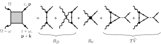
Figure 2: Feynman diagrams describing Raman scattering with the excitations of electron-hole pairs in the final state.

The probability for a photon to undergo inelastic scattering from the state $(\mathbf{q},q_{z})$ with energy $\Omega$ into a state $\mathbf{(\tilde{q}=q-k},\tilde{q}_{z})$ with energy $\tilde{\Omega}=\Omega-\omega$, by exciting an e-h pair in graphene with Fermi energy $\alpha\mu$ at low temperature $T<\omega$, is

$$w = \int\frac{d^{2}\mathbf{p}}{4\pi\hbar^{3}}f_{\mathbf{p}^{\eta\alpha}}(1-f_{(\mathbf{p+k)}^{\alpha}})\delta(\varepsilon_{\mathbf{p}^{\eta\alpha}}-\varepsilon_{(\mathbf{p+k)}^{\alpha}}+\omega)$$ (3)

$$\times\sum_{\xi}\mathrm{tr}\left\{R(1+\eta\alpha\boldsymbol{\Sigma}\mathbf{n}_{\mathbf{p}})R^{+}(1+\alpha\boldsymbol{\Sigma}\mathbf{n}_{\mathbf{p+k}})\right\}.$$

Here, $\alpha=\pm$  distinguishes between n- and p-doping of graphene, $\eta=-$/$+$ stands for the excitation of the inter/intra-band electron-hole pairs, and spin-degeneracy is taken into account. The probability $w$ describes the angle-resolved Raman spectrum, as opposed to the angle-integrated spectral density,

$$g(\omega)\equiv\frac{\Omega}{(2\pi\hbar)^{3}c^{2}}\int_{c|\mathbf{k}|<\Omega}\frac{w(\mathbf{k,}\omega)d^{2}\mathbf{k}}{\sqrt{\Omega^{2}-c^{2}\mathbf{k}^{2}}}.$$ (4)

In undoped graphene the inter-band e-h pairs are the only allowed electronic excitations. The probability,

$$w_{0}\approx\Xi_{s}\hbar e^{4}v^{2}\frac{\omega}{\Omega^{4}}+\frac{1}{2}\Xi_{o}\hbar e^{4}v^{2}\frac{\omega}{(6\gamma_{0}\Omega)^{2}},$$ (5)

$$\Xi_{s}=\left|\mathbf{l}\times\mathbf{\tilde{l}}^{\ast}\right|^{2},\qquad\Xi_{o}=1+(\mathbf{l}\times\mathbf{l}^{\ast})(\mathbf{\tilde{l}}\times\mathbf{\tilde{l}}^{\ast}),$$

of their excitation by photons with $\Omega<\gamma_{0}$ is dominated by the contribution, $R_{D}$ of the first two diagrams in Fig. 2. This determines typically crossed linear polarisation of in/out photons described by the polarisation factor $\Xi_{s}$, which is equivalent to saying that they have the same circular polarisation, in contrast to a weak contribution of the process enabled by the warping term (second term in Eq. (5)), with the opposite circular polarisation of in and out photons described by the factor $\Xi_{o}$.

In doped graphene, with $\mu\gg\Omega v/c$, inter-band electronic excitations with $\omega<2\mu$ are blocked, so that

$$w=w_{0}\times\begin{cases}\theta(\omega-2\mu),&\text{$|\omega-2\mu|>vk$;}\\ \frac{1}{\pi}\arccos\frac{2\mu-\omega}{vk},&\text{$|\omega-2\mu|<vk$.}\end{cases}$$ (6)

After integrating over all directions of the propagation of scattered photons, we find the spectral density of the angle-integrated Raman signal,

$$g(\omega)\approx\frac{1}{4}\Xi_{s}\left(\frac{e^{2}}{\pi\hbar c}\,\frac{v}{c}\right)^{2}\frac{\omega}{\Omega^{2}}F\left(\frac{\omega-2\mu}{\Omega v/c}\right).$$ (7)

Here $F(|x|<1)=\frac{1}{2}(1+x)$ and $F(|x|>1)=\theta(x)$, step function. In undoped graphene ($\mu=0$), spectral density $g(\omega)$ corresponds to the yield $I_{0}=\int_{0}^{\varpi}g(\omega)d\omega\sim\left(\frac{e^{2}}{hc}\,\frac{v}{c}\frac{\varpi}{\Omega}\right)^{2}$ such that $I_{0}(\varpi\sim\frac{1}{2}\Omega)\sim 10^{-10}$.

In doped graphene one may also expect to see some manifestation of the intra-band e-h excitations in the vicinity of the Fermi level, with a small energy transfer $\omega<\Omega v/c$. Their analysis requires taking into account all diagrams in Fig. 2, in particular, due to an additional asymmetry between the conduction and valence bands caused by the difference of their filling which increases the value of the triangular loop T ,

$$\mathcal{T}(\mu) = -(ev\hbar)^{2}\,(\mathbf{l}\cdot\mathbf{\tilde{l}}^{\ast})\,\frac{\mu\Pi}{\Omega^{3}};\quad\widetilde{V}=\frac{2\pi\hbar e^{2}}{k-2\pi\hbar e^{2}\Pi};$$

$$\Pi = \frac{2\mu}{\pi\hbar^{2}v^{2}}\frac{\omega-\sqrt{(\omega-i0)^{2}-v^{2}k^{2}}}{\sqrt{(\omega-i0)^{2}-v^{2}k^{2}}}.$$

Then, we find that, for $\omega\leqslant(v/c)\Omega\ll\Omega<\gamma_{0}$,

$$\delta g=\frac{1}{2}\left(\frac{e^{2}}{\pi\hbar c}\right)^{2}\frac{v}{c}\frac{\mu^{3}\omega}{\Omega^{5}}\Biggl{[}\left(\frac{v^{2}}{c^{2}}\Omega^{2}-\omega^{2}\right)\frac{\Omega^{2}}{8\mu^{4}}\Xi_{s}+\\ +\Xi_{o}\left(1+\frac{\Omega^{4}}{(6\gamma_{0}\mu)^{2}}\right)\Biggr{]}.$$

The yield of this low-energy feature is $\delta I=\int\delta g(\omega)d\omega\sim 10^{-15}$ for $\Omega\sim 1$eV Plasmon .

Electronic spectrum of graphene in a strong magnetic field can be described as a sequence $n^{\alpha}$ of Landau levels (LLs), $\varepsilon[n^{\alpha}]=\alpha\varepsilon_{n}$ with $\varepsilon_{n}=\sqrt{2n}\,\hbar v/\lambda_{B}$, corresponding to McClure ; AbergelFalko the states $|n^{\alpha}\rangle=\frac{1}{\sqrt{2}}(\Phi_{n},i\alpha\Phi_{n-1})$ for $n\geq 1$ and $|0\rangle=(\Phi_{0},0)$ (where $\lambda_{B}=\sqrt{\hbar c/eB}$ and $\Phi_{n}$ are the normalised LL wave functions in the Landau gauge). Then, electron’s Green functions and interaction vertices leading to optically active inter-LL excitations in monolayer graphene summarised in Table 2 take the form

$$\raisebox{-12.0pt}{\begin{picture}(28.0,28.0)(-14.0,-14.0)\put(-10.0,0.0){\line(1,0){20.0}} \put(0.0,0.0){\vector(1,0){4.0}} \end{picture}}= G^{R/A}=\frac{\delta_{nn^{\prime}}\delta_{\alpha\alpha^{\prime}}}{\varepsilon-\alpha\varepsilon_{n}\pm i0},$$

$$\raisebox{-12.0pt}{\begin{picture}(28.0,28.0)(-14.0,-14.0)\put(-8.0,12.0){\oval(8.0,8.0)[bl]} \put(-8.0,4.0){\oval(8.0,8.0)[tr]} \put(0.0,4.0){\oval(8.0,8.0)[bl]} \put(-8.0,8.0){\vector(1,-1){4.0}} \put(0.0,0.0){\line(1,1){12.0}} \put(8.0,8.0){\vector(-1,-1){4.0}} \put(0.0,0.0){\line(1,-1){12.0}} \put(5.0,-5.0){\vector(1,-1){4.0}} \put(0.0,0.0){\circle*{4.0}} \end{picture}}= \frac{ev\hbar}{2\sqrt{\Omega}}\mathbf{J}\cdot\mathbf{l},\quad\raisebox{-12.0pt}{\begin{picture}(28.0,28.0)(-14.0,-14.0)\put(-8.0,-12.0){\oval(8.0,8.0)[tl]} \put(-8.0,-4.0){\oval(8.0,8.0)[br]} \put(0.0,-4.0){\oval(8.0,8.0)[tl]} \put(-4.0,-5.0){\vector(-1,-1){4.0}} \put(0.0,0.0){\line(1,1){12.0}} \put(8.0,8.0){\vector(-1,-1){4.0}} \put(0.0,0.0){\line(1,-1){12.0}} \put(5.0,-5.0){\vector(1,-1){4.0}} \put(0.0,0.0){\circle*{4.0}} \end{picture}}=\frac{ev\hbar}{2\sqrt{\Omega}}\mathbf{J}\cdot\mathbf{\tilde{l}}^{\ast},$$

$$\mathbf{J}_{n^{\alpha}\,n^{\prime\alpha^{\prime}}} =\alpha i\delta_{n^{\prime},n-1}\mathbf{e}_{-}-\alpha^{\prime}i\delta_{n^{\prime}-1,n}\mathbf{e}_{+},$$

$$R_{w} =\frac{e^{2}v^{2}\hbar^{2}}{6\gamma_{0}\Omega}\Lambda^{z}\mathbf{J}\cdot\sum_{\pm}\mathbf{e}_{\pm}(\mathbf{le}_{\mp})(\mathbf{\tilde{l}}^{\ast}\mathbf{e}_{\mp}).$$

Here $\mathbf{e}_{\pm}=\frac{1}{\sqrt{2}}\left(\mathbf{e}_{x}\pm i\mathbf{e}_{y}\right)$ is used to stress that a circularly polarised photon carries angular momentum $m=\pm 1$.

The excitation of the e-h pairs by Raman scattering in graphene at strong magnetic fields characterised by the first two Feynmann diagrams in Fig. 2 produces the electronic transition $n^{-}\rightarrow n^{+}$ between LLs, with angular momentum transfer $\Delta m=0$ and excitation energy $\omega=2\varepsilon_{n}$ [Fig. 1], and transitions $(n-1)^{-}\rightarrow(n+1)^{+}$ and $(n+1)^{-}\rightarrow(n-1)^{+}$, with $\Delta m=\pm 2$ and $\omega=\varepsilon_{n-1}+\varepsilon_{n+1}$. The amplitudes of these two processes,

$$R_{n^{-}\rightarrow n^{+}}=\frac{1}{4}\frac{(ev\hbar)^{2}}{c^{2}\Omega}\times\\ \times\sum_{\alpha=\pm}\Biggl{[}\frac{(\mathbf{le}_{+})(\mathbf{\tilde{l}}^{\ast}\mathbf{e}_{-})}{\Omega-\varepsilon_{n}-\alpha\varepsilon_{n+1}}-\frac{(\mathbf{le}_{+})(\mathbf{\tilde{l}}^{\ast}\mathbf{e}_{-})}{\varepsilon_{n}-\Omega-\alpha\varepsilon_{n-1}}-\\ -\frac{(\mathbf{le}_{-})(\mathbf{\tilde{l}}^{\ast}\mathbf{e}_{+})}{\Omega\varepsilon_{n}-\alpha\varepsilon_{n+1}}+\frac{(\mathbf{le}_{-})(\mathbf{\tilde{l}}^{\ast}\mathbf{e}_{+})}{\varepsilon_{n}-\Omega-\alpha\varepsilon_{n-1}}\Biggr{]},$$

$$R_{(n\mp 1)^{-}\rightarrow(n\pm 1)^{+}}=\mp\frac{1}{4}\frac{(ev\hbar)^{2}}{c^{2}\Omega}(\mathbf{le}_{\pm})(\mathbf{\tilde{l}}^{\ast}\mathbf{e}_{\pm})\times\\ \times\sum_{\alpha=\pm}\Biggl{[}\frac{\alpha}{\Omega-\varepsilon_{n+1}-\alpha\varepsilon_{n}}+\frac{\alpha}{\varepsilon_{n-1}-\Omega-\alpha\varepsilon_{n}}\Biggr{]},$$

are such that $R_{n^{-}\rightarrow n^{+}}\gg R_{(n\mp 1)^{-}\rightarrow(n\pm 1)^{+}}$ for $\omega\ll\Omega$, due to a partial cancellation of the two diagrams constituting $R_{D}$. Notice that these inter-LL modes $n^{-}\rightarrow n^{+}$ have the symmetry of the representation A₂ in Table 1 and the same circular polarisation of in and out photons involved in its excitation. Finally, the contact term $R_{w}$ in Fig. 2 allows for a weak transition $n^{-}\rightarrow(n\pm 1)^{+}$, with the amplitude $R_{w}\ll R_{n^{-}\rightarrow n^{+}}$ NN1 . Superficially, such a transition, with $\Delta m=\pm 1$ resembles the inter-LL transition involved in the far-infrared (FIR) absorption Potemski2 ; AbergelFalko . However, the FIR-active excitation is ’valley-symmetric’ AbergelFalko and corresponds to the representation E₁, whereas the Raman-active $n^{-}\rightarrow(n\pm 1)^{+}$ mode corresponds to E₂, allowing the latter to couple to the $\Gamma$-point optical phonon and, thus, leading to the magneto-phonon resonance feature in the Raman spectrum Kechedzhi . Also, $R_{w}$ originates from the trigonal warping term in $\mathcal{H}$ which violates the rotational symmetry of the Dirac Hamiltonian by transferring angular momentum $\pm 3$ from electrons to the lattice, so that initial and final state photons in it have opposite circular polarisations.

C6v rep	transition	intensity	polarisation
E2	$\genfrac{}{}{0.0pt}{}{n^{-}\rightarrow(n+1)^{+}}{(n+1)^{-}\rightarrow n^{+}}$	weak in Raman, strong in magneto- phonon resonance	$\sigma^{\pm}\rightarrow\sigma^{\mp}$
E1	$\genfrac{}{}{0.0pt}{}{(n-1)^{-}\rightarrow(n+1)^{+}}{(n+1)^{-}\rightarrow(n-1)^{+}}$	weak in Raman	$\sigma^{\pm}\rightarrow\sigma^{\mp}$
A2	$n^{-}\rightarrow n^{+}$	dominant in Raman	$\sigma^{\pm}\rightarrow\sigma^{\pm}$

Table 2: Raman-active inter-LL excitations in graphene.

The dominant inter-LL transitions $n^{-}\rightarrow n^{+}$ determines the spectral density of light scattered from electronic excitations in graphene at high magnetic fields:

$$g_{n^{-}\rightarrow n^{+}}(\omega)\approx\Xi_{s}\left(\frac{v^{2}}{c^{2}}\frac{e^{2}/\lambda_{B}}{\pi\Omega}\right)^{2}\sum_{n\geq 1}\gamma_{n}(\omega-\omega_{n}).$$ (8)

Here $\gamma_{n}(x)=\pi^{-1}\Gamma_{n}/[x^{2}+\Gamma_{n}^{2}]$, and $\Gamma_{n}$ is inelastic LL broadening which increases with the LL number, $\omega_{n}=2\varepsilon_{n}=2\sqrt{2n}\hbar v/\lambda_{B}$, and the factor $\Xi_{s}=|\mathbf{l}\times\mathbf{\tilde{l}}^{\ast}|^{2}$ in Eq. (8) indicates that in and out photons have the same circular polarisation.

The $n^{-}\rightarrow n^{+}$ inter-LL transitions are specific for Dirac-type electrons in graphene and represent the most pronounced signature of its electronic excitations in the Raman spectrum. The quantum efficiency of the lowest, $\omega_{1}=2\sqrt{2}\hbar v/\lambda_{B}$ peak in the spectrum in Fig. 1 is $I_{1}\sim\left(\frac{v^{2}}{c^{2}}\,\frac{e^{2}/\lambda_{B}}{\pi\Omega}\right)^{2}$ per incoming photon. For $B=20$T, we estimate $I_{1}$ $\sim 10^{-12}$ for photons with energies in the visible range, which is feasible to detect in the inelastic light scattering experiments.

We thank I. Aleiner, D. Basko, A. Ferrari, A. Geim, A. Pinczuk, and M. Potemski for useful discussions. We acknowledge financial support from EPSRC grants EP/G014787, EP/G035954 and EP/G041954.

References

(1) W. Weber and R. Merlin (Eds.), Raman Scattering in
Materials Science, Springer Series in Materials Science, Vol. 42, Springer
2000.
(2) A.C. Ferrari, et al, Phys. Rev. Lett. 97, 187401 (2006).
(3) D. Graf, et al, Nano Lett. 7, 238 (2007).
(4) L.M. Malard, et al, Phys. Rev. B 76,
201401(R) (2007).
(5) J.W. Jiang, et al, Phys. Rev. B 77, 235421
(2008).
(6) C. Faugeras, et al, Appl. Phys. Lett. 92, 011914 (2008).
(7) S. Berciaud, et al, NanoLett. 9, 346
(2009).
(8) I. Calizo, et al, arXiv:0903.1922
(9) D.M. Basko, Phys. Rev. B 78, 125418 (2008); Phys.
Rev. B 76, 081405 (2007)
(10) S. Pisana, et al, Nature Mat. 6,
198 (2007).
(11) A.H. Castro Neto and F. Guinea, Phys. Rev. B 75, 045404 (2007).
(12) T. Ando, J. Phys. Soc. Jpn. 76, 024712 (2007).
(13) M.O. Goerbig, et al, Phys. Rev. Lett. 99, 087402 (2007).
(14) J. Yan, et al, Phys. Rev. Lett. 98,
166802 (2007).
(15) J. Yan, et al, Phys. Rev. Lett. 101,
136804 (2008).
(16) D.M. Basko, S. Piscanec, A.C. Ferrari, arXiv:0906.0975
(17) M.L. Sadowski, et al, Phys. Rev. Lett. 97, 266405 (2006).
(18) Z. Jiang, et al, Phys. Rev. Lett. 98, 197403
(2007).
(19) A.B. Kuzmenko, et al, Phys. Rev. B 79,
115441 (2009).
(20) L.M. Zhang, et al, Phys. Rev. B 78, 235408
(2008).
(21) D.S.L. Abergel and V.I. Fal’ko, Phys. Rev. B 75, 155430 (2007).
(22) P. Blake, et al, Appl. Phys. Lett. 91,
063124 (2007).
(23) D.S.L. Abergel, A. Russell, and V.I. Fal’ko,
Appl. Phys. Lett. 91, 063125 (2007).
(26) P.M. Platzmann and P.A. Wolff, Waves and
interactions in solid state plasmas, Academic Press, New York 1973.
(27) Contact interaction has been considered in
Ref. Chinese1 as the dominant Raman scattering mechanism in graphene.
Such an assumption is justified for scattering of soft X-rays with
energies eV larger than the bandwidth in
this material. However, as shown here, for photons
in the visible range (with energies eV)
such an assumption would lead to incorrect
symmetry of the excitations, polarisation properties of the Raman signal,
and selection rules for the dominant inter-LL excitations.
Although for a zero magnetic field the spectral density of inelastically
scattered light found in Ref. Chinese1 and in the present study may
look similar, which is because it coincides with the density of state of
zero-momentum electron-hole excitations in graphene, the use of contact interaction
alone underestimates the intensity of Raman scattering of visible
light by two orders of magnitude.However, such term is important to take into account
(among many others Basko2 ) in the analysis of the quantum efficiency of the excitation
of the -point optical phonon.
(28) H.-Y. Lu and Q.-H. Wang, Chinese Physics Letters 25, 3746 (2008).
(31) R. Saito, G. Dresselhaus, M.S. Dresselhaus, Physical Properties of Carbon Nanotubes, Imperial College Press, London
1998.
(32) E. McCann et al, Phys. Rev. Lett. 97,
146805 (2006).
(33) K. Kechedzhi et al, Eur. Phys. J. ST 148, 39
(2007).
(34) The value of is sensitive to the
conduction-valence band asymmetry. For a symmetric spectrum
since two ‘triangles’ with the opposite direction cancel each other. Using
the two-band tight-binding model Dresselhaus with asymmetry in the
spectrum is taken into account through is the nearest-neighbor overlap
integral , we estimate ( is lattice constant). Using , we find that . Note that no
resonantly enhanced contribution towards comes from virtual
states with , since, after the integration over
intermediate states, the contributions of pairs of poles in the products of
Green’s functions in cancel each other.
(35) E.H. Hwang and S. Das Sarma, Phys. Rev. B 75,
205418 (2007).
(36) Doped graphene also has collective low-energy modes:
plasmons DasSarma with . Taking into account the plasma pole of the propagator in , we estimated the
probability of the plasmon emission as and quantum efficiency .