Universal Correlations and Power-Law Tails
in Financial Covariance Matrices

Abstract

Signatures of universality are detected by comparing individual eigenvalue distributions and level spacings from financial covariance matrices to random matrix predictions. A chopping procedure is devised in order to produce a statistical ensemble of asset-price covariances from a single instance of financial data sets. Local results for the smallest eigenvalue and individual spacings are very stable upon reshuffling the time windows and assets. They are in good agreement with the universal Tracy-Widom distribution and Wigner surmise, respectively. This suggests a strong degree of robustness especially in the low-lying sector of the spectra, most relevant for portfolio selections. Conversely, the global spectral density of a single covariance matrix as well as the average over all unfolded nearest-neighbour spacing distributions deviate from standard Gaussian random matrix predictions. The data are in fair agreement with a recently introduced generalised random matrix model, with correlations showing a power-law decay.

1 Introduction

’Econophysics’, a hybrid of ’economy’ and ’physics’, has become a very active field of research in the past decade. In this paper we will focus on aspects of portfolio selection and market modelling. In particular we will analyse cross-correlations in financial time-series and compare to the predictions of Random Matrix Theory (RMT). We refer to the reviews [1, 2] on this subject, as well as for other methods e.g. from field theory to [3].

A still debated issue in the community is to what extent the ’historical’ determination of covariance estimators (i.e. based on past time-series over a finite temporal window $T$) can be trusted when forecasting the financial risk of a certain portfolio; put it differently, how reliably is the past going to shape the future? In a pioneering paper, Laloux et al. [4] used a comparison with RMT to cast serious doubts on the usefulness of historical covariance spectra in estimating the variance (and thus the future risk) of a given portfolio, questioning the widely applied procedure of Markowitz’s theory based on Gaussian mean-field approximations. The ’measurement noise’ due to the finiteness of the historical time series $T$ was claimed in [4] to bury most of the relevant information encoded in the historical covariance matrices, thus impairing ab ovo much of the consequent predictions. In subsequent papers the work of [4] was repeated and refined to other quantities, using Gaussian RMT [5, 6, 7, 8], non-Gaussian heavy tailed distributions [9, 10, 11, 12, 13, 14, 15], or RMT with complex eigenvalues using lagged time series [16, 17]. In addition clever methods were devised to detect meaningful correlations buried under the ’noise-dressed’ regions of the spectra [18, 19], thus trying to mitigate the pessimistic forecast of [4].

A central tool for our comparison with empirical financial data is the so-called Wishart-Laguerre (WL) ensemble of random matrices. The WL ensemble contains random matrices of the form [20] $\mathbf{W}=(1/T)\mathbf{X}^{\dagger}\mathbf{X}$, where $\mathbf{X}$ is a rectangular matrix of size $T\times N~{}$($T>N$), whose entries are independent Gaussian variables in the simplest case, and $\mathbf{X^{\dagger}}$ is the Hermitian conjugate of $\mathbf{X}$. As such, the WL ensemble contains (positive definite) covariance matrices $\mathbf{W}$ of maximally random data sets. They have since appeared in many different contexts apart from quantitative finance, ranging from mathematical statistics [21] and statistical physics [22] to gauge theories [23], quantum gravity [24] and telecommunications [25].

By definition, the WL ensemble constitutes a ’null hypothesis’, with the highest degree of randomness and lowest degree of built-in information in the data-set, and therefore is an ideal benchmark for comparison with the a priori much richer correlations in the financial time series.

Within the large-$N$ predictions of WL one has to distinguish between global spectral properties, taking into account correlations over a scale of $O(1)$ much larger than the mean level spacing, and local properties, probing correlations on the scale of the mean spacing (typically of $O(1/N)$). It is well known that the latter are much more robust under small deformations of the Gaussian probability distribution of the matrix elements. Typical examples include the distribution of individual eigenvalues and individual spacings among eigenvalues in the bulk.

While the global spectral density has received a good deal of attention in the works quoted above, the spacing distribution has so far only been investigated in [5, 6], histogramming the spacings between all consecutive eigenvalues after unfolding. One of the aims of this paper is to further investigate the local statistics (individual distributions), taking also into account the presence of non-Gaussian heavy tails in the spectral density.

In order to test e.g. if the smallest eigenvalue follows the universal Tracy-Widom distribution [26], as was proven only very recently for WL with real matrix elements [27], we immediately face the following problem: a single covariance matrix clearly does not allow for testing individual eigenvalue distributions. We are therefore led to define a meaningful way of generating ensembles of covariance matrices from a single data set. These are then tested against WL and its generalisation with power-law tails that was proposed in [28] and further developed for local statistics in [13] as well as in this paper.

This article is organised as follows. In section 2 we summarise the relevant predictions from RMT, both for the standard WL ensemble and its non-Gaussian generalisation with power-law tails. In section 3 we compare these to data from financial covariance matrices. This section is divided into two parts. In 3.1 we compare to the data from a single covariance matrix partly repeating previous analysis. In the second subsection 3.2 we define ensembles of matrices by chopping the covariance matrix, and compare to the distribution of individual eigenvalues and spacings. In section 4 we offer some conclusions, followed by 3 appendices containing technical details and consistency checks.

2 Random Matrix Predictions

In this section we summarise the analytical predictions from RMT, both for the standard Gaussian model and its generalisation. We do not give derivations here but rather illustrate these predictions by comparing to numerically generated random matrices for both models.

2.1 Global density and level spacing

We first introduce the standard Wishart-Laguerre (WL) ensemble of Gaussian random matrices (also called chiral Gaussian ensemble). In view of our application to time series, in particular stock price fluctuations, we restrict ourselves to real matrix elements denoted by the Dyson index $\beta=1$. Its probability density distribution of matrix elements is given by

$${\cal P}_{{W\!L}}\left(\mathbf{X}\right)\sim\exp\left[-\sigma^{2}{\mbox{Tr}}(\mathbf{X}^{T}\mathbf{X})\right],$$ (2.1)

where X is a matrix of size $T\times N~{}$ ($T>N$) with real elements. The integration measure $d\mathbf{X}$ is defined by integrating over all independent matrix elements of X with a flat measure. The joint probability distribution of the positive definite eigenvalues of $\mathbf{W}=(1/T)\mathbf{X^{\dagger}}\mathbf{X}$ (the so-called Wishart matrix), or equivalently the singular values of the matrix $\mathbf{X}$ is obtained by integrating over the angular degrees of freedom. Since we are only interested in two specific correlation functions in the large-$N$ limit we give the results without derivation.

The global spectral density defined as $\rho(\lambda)=\langle{\mbox{Tr}}~{}\delta(\lambda-\mathbf{W})\rangle$, averaged with respect to (2.1). In the large-$N$ limit it is given by [29]

$$\rho_{M\!P}(x)=\ \frac{1}{2\pi cx}\sqrt{(x-cX_{-})(cX_{+}-x)}\ ,\ \ \mbox{with}\ \ x\in[cX_{-},cX_{+}]\ .$$ (2.2)

This is called Marčenko-Pastur law, and we have normalised it to have integral and first moment equal to unity (see e.g. fig 4). The endpoints of support are

$$X_{\pm}\ \equiv\ (c^{-\frac{1}{2}}\pm 1)^{2}\ ,$$ (2.3)

where both the large-$N$ and large-$T$ limit is taken with $N=cT$, keeping $0<c\leq 1$. Indeed, the applications to times series analysis require $T$ to be much larger than the number of stocks $N\ll T$.

A second quantity of interest is the spacing distribution between consecutive levels in the bulk of the spectrum, probing correlations on a local level of order $O(1/N)$. We make a distinction between global and individual nearest-neighbour distributions. The former is obtained by averaging over spacings in the bulk after unfolding (see appendix C) and is commonly used in comparisons to RMT. The latter is defined as the distribution of the spacing $s_{k}$ between the $k$th and $(k-1)$st eigenvalue, for fixed $k$ and $N$ (see e.g. [30]):

$$s_{k}=\frac{\lambda_{k}-\lambda_{k-1}}{\langle\lambda_{k}-\lambda_{k-1}\rangle}\ ,$$ (2.4)

and it provides information about local correlations at a given point in the bulk, without making any further assumptions.

Within RMT the global and individual spacing in the bulk agree, and an excellent approximation for both distributions can be obtained by applying the so-called Wigner surmise (WS), based on a $2\times 2$ matrix calculation. As was explained and checked numerically in [14], the correct surmise for WL is obtained from the Wigner-Dyson (or Gaussian) ensembles (see also [5, 6])

$$p_{W\!D}(s)=\frac{\pi}{2}s\ \exp\left(-\frac{\pi}{4}s^{2}\right)\ ,$$ (2.5)

here for $\beta=1$. It has norm and first moment of unity. Eqs. (2.2) and (2.5) are very well known and have been compared to financial data in previous works (see e.g. [4, 7, 8, 31] and [5, 6] respectively).

We now turn to the recent generalisation of WL introduced in [28, 13]. It can be derived from a superstatistical or generalised entropy approach, representing an interpolation between the fully chaotic or random statistics of the Gaussian WL, and a regular or integrable behaviour. The generalisation of the probability distribution of matrix elements eq. (2.1) reads

$${\cal P}_{\alpha}\left(\mathbf{X}\right)\sim\left(1+\frac{1}{\alpha+\frac{1}{2}NT+1}{\mbox{Tr}}(\mathbf{X}^{T}\mathbf{X})\right)^{-(\alpha+\frac{1}{2}NT+1)},\ \ \alpha>0\ ,$$ (2.6)

where the $N$-dependence is required by convergence. The resulting global density that generalises the Marčenko-Pastur density eq. (2.2) is reading [28]

$$\rho_{\alpha}(x)\ =\ \frac{1}{2\pi c\alpha\Gamma(\alpha+1)}\left(\frac{c\alpha}{x}\right)^{\alpha+2}\int_{X_{-}}^{X_{+}}dt\,t^{\alpha}\exp\left[-\frac{c\alpha}{x}\,t\right]\sqrt{(t-X_{-})(X_{+}-t)}\ ,$$ (2.7)

and it displays a power law tail [13]. The density is normalised to unity and has first moment equal to one (see fig. 4 for illustration). The integral can be computed in terms of a confluent hypergeometric series [13]. For large arguments the density decays algebraically as $\rho_{\alpha}(x\gg 1)\sim x^{-\alpha-2}$. For small arguments the density is suppressed exponentially, and for a more detailed discussion we refer to [13]. The standard WL quantities are recovered when $\alpha\to\infty$.

In complete analogy with the standard WL ensemble, we can define the spacing distribution for the generalised ensemble eq. (2.6) that generalises eq. (2.5). It is based on a Wigner surmise for the corresponding generalised WD ensemble (see also [32]). Although this quantity was not derived in [13], it follows in analogy to the corresponding quantity in [14] where generalisations of (2.5) with (stretched) exponential tails were considered. We shall therefore be brief and only quote the answer for $\beta=1$ relevant here:

$$p_{\alpha}(s)=\frac{\pi s}{2\alpha^{2}\Gamma(\alpha+1)}\int_{0}^{\infty}dt\,t^{\alpha+2}\exp\left[-t-\frac{\pi t^{2}}{4\alpha^{2}}\,s^{2}\right]\ .$$ (2.8)

The norm and first moment are again chosen to be unity. Exploiting the solution of the integral in terms of Hypergeometric functions it is easy to see that the local spacing distribution decays with the same power as the global density eq. (2.7), $p_{\alpha}(s\gg 1)\sim s^{-\alpha-2}$. A saddle point evaluation confirms that (2.8) reproduces (2.5) as expected when $\alpha\to\infty$.

We have verified numerically that the generalised spacing distribution (2.8) indeed agrees with individual spacings (eq. (2.4)) from random matrices from eq. (2.6). This is shown in fig. 1.

In both ensembles the results given so far, the global density and the global spacing, can be tested on a single realization of a random or data matrix. For individual spacings as well as for the distribution of individual eigenvalues we need an ensemble of matrices, and the predictions for the latter are given in the next subsection.

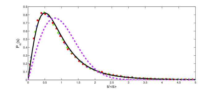
Figure 1: Test of the large-$N$ individual spacing distribution in the generalised WL model eq. (2.8) (full line) vs. the individual spacing distributions (2.4) for $k=4,6,8$ at $N=8$, $T=16$ and $\alpha=3$, from numerically generated random matrices with distribution (2.6). The spacing distribution for the standard WL Eq. (2.5) is added for comparison (pink dashed line).

2.2 Smallest and largest eigenvalues

For the Gaussian WL ensemble with real matrix entries, both the distributions of the largest and smallest eigenvalue have been rigorously studied by Johnstone [21], and very recently by Feldheim and Sodin [27], respectively. In a well defined scaling limit both cases follow a Tracy-Widom (TW) [26] distribution $F_{1}(s)$. More precisely, there exist $N$-dependent constants $a_{N}^{(L)},b_{N}^{(L)},a_{N}^{(S)},b_{N}^{(S)}$ such that

$$\mbox{Prob}[\chi_{{\rm min}({\rm max})}<x]=F_{1}(x)$$ (2.9)

where we have introduced the following scaled random variables:

$$\chi_{{\rm min}} =\ \frac{a_{N}^{(S)}-\lambda_{{\rm min}}}{b_{N}^{(S)}}\ ,$$ (2.10)

$$\chi_{{\rm max}} =\ \frac{\lambda_{{\rm max}}-a_{N}^{(L)}}{b_{N}^{(L)}}\ .$$ (2.11)

The Tracy-Widom distribution $F_{1}(x)$ defined in eq. (2.9) is given by

$$F_{1}(x)\equiv\exp\left[-\int_{x}^{\infty}ds\Big{(}q(s)+(s-x)q(s)^{2}\Big{)}\right]$$ (2.12)

where $q(s)$ is the solution to the second Painlevé equation (PII)

$$q(s)^{\prime\prime}=sq(s)+2q(s)^{3}$$ (2.13)

subject to the boundary condition of approaching the Airy function asymptotically, $q(s)\sim\mbox{Ai}(s)$ for $s\to\infty$. This is also called the Hastings-McLeod solution of PII.

As an independent check we have generated real WL matrices and compared the numerical distribution for the smallest and largest eigenvalues to $F_{1}(x)$, see figure 2.

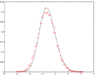
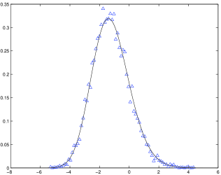
Figure 2: The distribution of the smallest (left) and largest (right) eigenvalues for $\beta=1$ WL, after centring and the rescalings eqs. (2.10) and (2.11). The full line corresponds to the theoretical curve eq. (2.12), the points originate from 60000 numerically generated WL matrices of size $N=80$ and $T=320$. To generate efficiently TW densities, see [33].

The result for the largest and smallest eigenvalues given so far is valid for the standard, Gaussian WL ensemble. Because of the implicit nature of the TW distribution, we have not managed to analytically derive the corresponding distribution valid for the generalised ensemble (2.6) with power law tails. In related models about the generalised WD class it was argued [34, 35] that a transition between TW and the Fréchet or normal distribution takes place for the largest eigenvalue.

Here, instead we have numerically produced the distribution of the smallest and largest eigenvalue in the generalised ensemble and observed the expected convergence to the WL distribution when $\alpha$ gets large, see fig. 3. Because we do not know the modification of the scaling relation in the generalised WL ensembles we show the unscaled data.

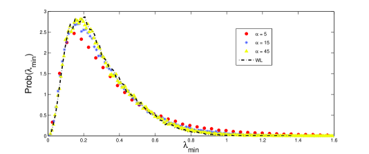
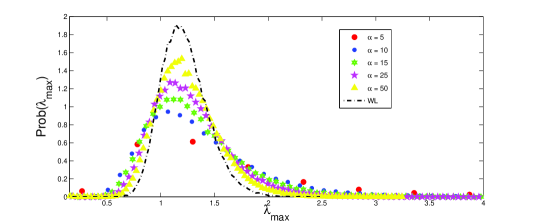
Figure 3: Distribution of the unscaled smallest (left) and largest (right) eigenvalues for the generalised ensemble eq. (2.6) for the case $N=8$, $T=15$ and different values of $\alpha$. For comparison the corresponding distribution for the WL ensemble (dash-dotted black line) is given, which after a proper rescaling (eqs. (2.10) and (2.11)) maps to fig. 2.

An important observation we make is that the distribution of the largest eigenvalue is strongly modified due to the power law tail of the spectrum. In contrast the smallest eigenvalue undergoes only a mild modification. This is probably because the exponential suppression of the spectral density at the lower “pseudo” edge is not dramatically different from the square root edge in WL. This will be important when comparing to data in the next section.

3 Comparison to Financial Correlation Matrices

In this section, we compare the RMT predictions from the previous section to data from financial covariance matrices. Our motivation with respect to previous works has been two-fold.

First, can we improve the fit of financial spectra to the global MP density of eigenvalues following the null-hypothesis of Gaussian random variable by introducing correlations among matrix elements that lead to power-law tails? A similar route has been followed previously in [12] albeit with a different model; our model and a first comparison was given in [13].

Second, can we test RMT predictions that are more robust under deformations of the Gaussian measure of WL than the MP density? The quantities we have looked at are the individual and global spacing distribution for standard WL, and the individual distribution of the smallest eigenvalue. The individual distributions of course require the definition of a suitable ensemble of homogeneous matrix objects to average over. The global spacing distribution was previously compared to data in [5, 6].

In the first subsection 3.1, we focus on quantities that can be inferred from a single financial covariance matrix, whereas in the second subsection 3.2 we define a new chopping procedure to generate ensembles of covariance matrices from one single instance in order to analyse the individual eigenvalue statistics.

3.1 Power-law decay in the global density and the global spacing

In this subsection we have analysed a single set of data given by $N=401$ stocks and a time series of daily prices $T=970$. The data were obtained from the S&P 500 Equity Index. It is representative of the U.S. equity market and hence of their economy including the 500 largest companies. We extracted the daily opening prices for the 4-year period 2002-2006. Stocks that did not survive in the index during that period were deleted from the analysis, hence the reduced number of 401 stocks. Henceforth we will refer to this dataset as set SP.

The financial covariance matrix is obtained in the standard way [4] which we briefly recall. First the normalised return $G_{i}(t)$ of the $i$-th stock at time $t$ is computed as the following function of its stock price $S_{i}(t)$

$$G_{i}(t)=\log[S_{i}(t+\Delta t)]-\log[S_{i}(t)]\ ,$$ (3.1)

where the time step $\Delta t$ is 1 day for our set SP. Then the temporal mean $\langle G_{i}(t)\rangle$ and variance $\sigma_{i}$ are computed for each stock independently to give the normalised data matrix elements

$$X_{it}=\frac{G_{i}(t)\ -\ \langle G_{i}(t)\rangle}{\sigma_{i}}\ .$$ (3.2)

Clearly the $X_{it}$ over the period $t=1,\ldots,T$ have variance one and vanishing mean. Then the eigenvalues of the covariance matrix $\mathbf{C}=(1/T)\mathbf{X}^{T}\mathbf{X}$ of these data are computed and histogrammed in fig 4. The spectral density obtained in this fashion is normalised to unity and rescaled to have a first moment equal to $1$. It can then be compared to the MP density (2.2) which is parameter free under the same rescaling, and to the generalised density in (2.7). In previous works using the standard Gaussian WL ensemble a one-parameter fit was performed using a variance dependent MP density, arguing that the outlying eigenvalues with respect to RMT would effectively reduce the inverse variance $\sigma$ in eq. (2.1) [4]. No such freedom is left in our approach as the first moment has been already normalised to $1$.

The resulting agreement between the generalised density (2.7) and the data is very good after fitting the only free parameter $\alpha\approx 0.95...$ in the generalised model. This leads to a power-law decay with exponent $\alpha+2\approx 2.95$. It has been observed independently in the framework of a similar model [12] that the global spectral histogram is better fitted by a density with power-law tails rather than MP. Despite many differences between the two models, the exponent $2.93$ found in [12] is similar to ours, using a very similar set of data (daily returns of from S&P 500 Equity Index from 2003-2007).

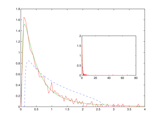
Figure 4: Comparison between part of the rescaled eigenvalue distribution from financial data set SP, and the macroscopic density $\rho_{\alpha}(x)$ from RMT for the generalised model eq. (2.7), in red and green respectively. The best fit gives a value of $\alpha\approx 0.95$, which corresponds to a power-law decay as $\rho_{\alpha}(x)\sim x^{-2.95}$. For comparison we have added the parameter free MP density eq. (2.2). The inset shows all eigenvalues on a different scale.

A second quantity we analyse is the nearest-neighbour spacing distribution which resolves local information of the order $O(1/N)$ and is much more universal, being the Fredholm determinant of the universal sine-kernel [36]. For a detailed discussion of universality issues we refer to [13].

In this subsection we specifically look at the global level spacing distribution, obtained from a single sequence of sorted eigenvalues (one matrix sample).

After unfolding the spectrum, a standard procedure in RMT [37] where we use a polynomial fitting of the cumulative eigenvalue distribution (see appendix C for details), the normalised histogram of all spacings between consecutive eigenvalues is plotted in fig. 5. Note that we have made an important assumption here: we assumed that averaging over the spacings between different consecutive eigenvalues of a single covariance matrix converges to a single distribution function after unfolding. Whereas in RMT this is known to hold due to the self-averaging property (or ergodicity) this is by no means guaranteed for financial covariance matrices.

The result in fig. 5 shows that the spacing distribution seems to deviate from the WS of standard WL, although our statistics is not extremely good. This is in contrast with previous analysis [5, 6] where a good agreement with WS was found . For comparison we give our generalised spacing distribution eq. (2.8): from the value $\alpha=0.95$ as determined in fig. 4 we get a worse fit than from the WS. However, using $\alpha$ as a free fitting parameter the apparently best fit is given by the generalised spacing for $\alpha\approx 8$, thus parametrising the deviation from WL. This can be interpreted as the system not being fully random, as we have seen from the global spectrum.

Because our statistics is not very good we will come back to this question at the end of the next subsection 3.2. The ensembles from a chopped covariance matrix show the same effect more clearly.

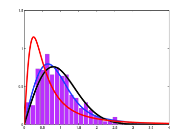
Figure 5: The unfolded global spacing distribution from financial data set SP vs the RMT prediction eq. (2.5) for WL (black right curve), and eq. (2.8) for our generalised ensemble: $\alpha=0.95$ (red left curve) and the best fit with $\alpha=8$ (blue middle curve).

3.2 Universal individual eigenvalue distributions

In this section we analyse the distribution of individual eigenvalues and spacings and compare them to the universal TW and WS distributions respectively (and their generalisation). In order to generate ensembles of covariance matrices we use two different methods here:

Method 1: We take a long time series $T$ of a small number $N$ of stocks, and then chop $T$ into $\ell$ smaller time windows of equal length $t$, $T=\ell t$. This creates an ensemble of $\ell$ covariance matrices of size $t\times N$ of the same $N$ stocks, with $c=N/t\in(0,1]$.

Method 2: We take a time series $T$ of $N$ stocks, and chop both $N$ into $k$ sets of $n$ stocks, with $N=kn$, as well as chopping $T$ into $\ell$ smaller time windows of equal length $t$, $T=\ell t$, as before. This creates an ensemble of $k\ell$ covariance matrices of size $t\times n$, thus mixing different sets of $n$ stocks, with $c=n/t\in(0,1]$.

While the chopping in smaller time windows in method 1 (and 2) is unambiguous - apart from choosing the length of the time window $t$ - the chopping into smaller subsets of stocks may seem at first quite hazardous, mixing in an arbitrary way fairly heterogeneous data. Surprisingly, we find the same universal properties from both methods.

To test the consistency of method 2 we have produced ensembles of the same size using several choppings and including different subsets of stocks (see appendix B), and we detected a substantial robustness of ensemble properties with respect to random reshuffling. A clear advantage of method 2 is that we can produce a much better statistics. Furthermore we have varied the length on the time window $t$ in both method 1 and 2. Here we have taken care to choose $t$ (and $n$) such that the resulting value $1/c$ remains bounded of the order $O(10)$, in order to avoid the problems discussed in [31] for large ratios.

We begin by using ensembles generated from method 1. This is done with our second data set DJ based on the Dow-Jones Index obtained as follows. Daily returns for $N=27$ stocks were used in the time interval from June 1997 to October 2005, leading to a $T=17109$. From this we have created an ensemble of 179 (356) correlation matrices of size $96\times 20$ ($48\times 20$). Our choice was motivated by having some data with the same $c$-value as from method 2 below.

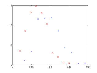
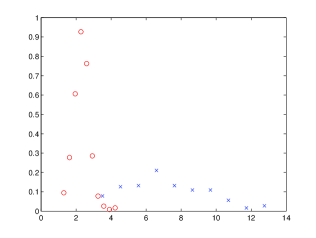
Figure 6: Method 1 using data set DJ and the ensemble $48\times 20$. Left plot: superposition of the smallest (red circles) and second smallest eigenvalue (blue crosses). Right plot: superposition of the second largest (red circles) and largest eigenvalues (blue crosses).

The full spectrum is given in fig. 11 in appendix A, but we shall focus on the local properties here. The result for the unscaled first and second eigenvalue is given in fig. 6 left. The spacing between the two (as well as their individual widths) are of the order of the mean level spacing $1/N\approx 0.05$. This indicates that a comparison to the TW prediction from RMT (and its generalisation) is meaningful.

For comparison we also give the distribution of the largest and second largest eigenvalue from method 1 in fig. 6 right. Obviously the shape and width are very different, and the spacing is much larger than $1/N$. Already the second largest eigenvalue is within the support of both the MP and generalised density, see fig. 11 of the full spectrum in appendix A. From previous considerations [4] as well as our previous section 3 one could speculate whether or not the largest eigenvalues are non-random, containing information.

Because in the WL ensembles TW describes both the smallest and the largest eigenvalues we could try to compare these predictions with the data. However, there are some hints that such a program is essentially ill-defined, due to the absence of a clear-cut separation between eigenvalues following RMT statistics and those carrying genuine information. The fact that we find a fit better fit to our generalised RMT with power law tails makes this even more difficult. On the other hand it has been argued in [18] that information could be extracted from underneath the density close to the right edge, using a power mapping method.

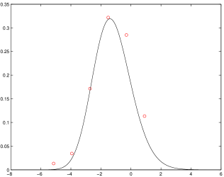
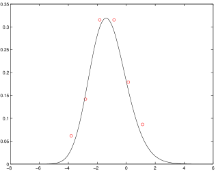
Figure 7: The rescaled smallest eigenvalue from method 1 using data set DJ. Left: ensemble of size $48\times 20$. Right: ensemble of size $96\times 20$.

For these difficulties we have fitted only the smallest eigenvalue with the TW distribution, with the result given in fig. 7. As was discussed in the previous subsection 3.1 we only expect minor deviations for the smallest eigenvalue in our generalised ensemble eq. (2.6). Although we only have a few points in the plot, we can at least conclude that the data are consistent with at fit to TW (as well as our generalised model). Note that this finding is invariant under doubling the size of the temporal windows, fig. 7 left vs right.

The TW distribution is well know to be strongly universal within RMT, being invariant under non-Gaussian deformations of the probability distribution eq. (2.1), by adding higher order terms in the exponent. We have therefore established that a trace of this universality is also seen in ensembles of financial covariance matrices.

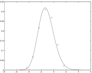
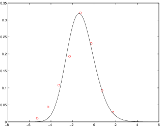
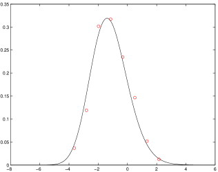
Figure 8: The rescaled smallest eigenvalue from method 2 using data set SP. Left: ensemble of size $48\times 10$, middle $48\times 20$, right: $96\times 20$.

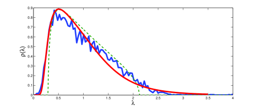
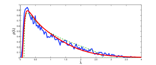
Figure 12: Comparison between part of the global spectral density from ensembles using method 2 on data set SP: the $48\times 10$ chopped ensemble (left) and $48\times 20$ (right) vs the generalised density eq. (2.7) (full red line) for $\alpha=7,8$ respectively. The MP distribution eq. (2.2) (dashed line) gives a worse fit.

We can now repeat the same analysis using method 2. Here we reuse the data set SP from the previous subsection 3.1, and chop the $970\times 401$ matrix into ensembles of submatrices of various sizes. The full densities for submatrix size $48\times 10$ and $48\times 20$ of respective ensemble sizes 800 and 400, are shown in appendix A fig. 12. The situation for the distribution of the first vs second, as well as largest vs second largest eigenvalue is similar as in method 1 described above, and we refer to appendix B for details. The fit to the universal TW distribution using method 2 is shown in fig. 8, with the same conclusion as above. Here we have halved the chopping size in $n$ (stock) direction, as well as doubled the time window $t$, which all lead to consistent fits.

In appendix B we also compared the distribution of the smallest eigenvalues for a fixed sub-matrix size $48\times 20$, choosing different subsets of 20 stocks out of 400. Because the unscaled first eigenvalues lie on top of each other we do not repeat the rescaled fit to TW for these permutations. We have also analysed other sub-matrix sizes, and we have subpartitioned the data set DJ using method 2 as well. In all cases we obtained approximately the same level of consistency.

We now move to the second local quantity, the individual spacing distributions for our ensembles as described in eq. (2.4). Because of better statistics we restrict ourselves to ensembles generated from method 2. Since we are dealing with individual spacings, no unfolding is necessary here. All distributions are consistent with the WS eq. (2.5) relevant for the unperturbed WL ensembles. We do not find any trace here from our generalised ensemble, in spite of its better fit of the full density, see fig. 12.

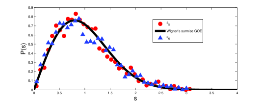
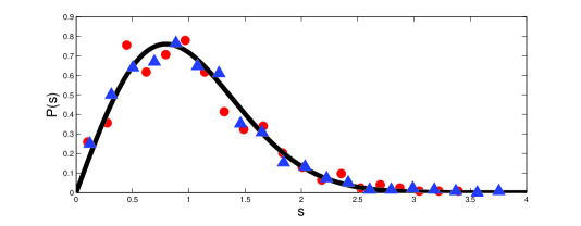
Figure 9: The WS eq. (2.5) vs the distribution of two individual spacings in the middle of the spectrum: 5th and 6th spacing of 10 eigenvalues, for ensembles of size $24\times 10$ (left) and $48\times 10$ (right) from method 2.

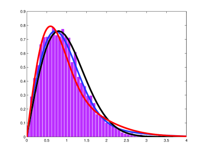
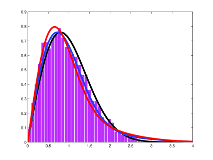
Figure 10: The WS eq. (2.5) vs the global spacings distribution, for ensembles of size $48\times 10$ (left) and $48\times 20$ (right) from method 2. The generalised surmise is displayed with the values $\alpha=7,8$ extracted from the global density in fig. 12 respectively, and with the best fitted value of $\alpha=9$ in both cases.

Let us return to the question of a deviation from the WS for the global spacing distribution from the previous subsection 3.1. Repeating the same analysis by unfolding the chopped data from method 2 and then averaging over all consecutive spacings we again find a deviation from the WS in the global spacing distribution, but with a much clearer signal compared to fig. 5.

As in fig. 5 we compare the WS and the generalised spacing eq. (2.8). Like before the $\alpha$-value determined from the global spectral density, see fig. 12, does not give the best fit (although it is not as bad as in fig. 5). Using $\alpha$ as a free fit parameter we can clearly give a much better fit than the WS. This may again be seen as an indication that the data are not fully random.

4 Conclusions

We have studied the spectral properties of empirical covariance matrices from financial data, by comparing to the predictions of two different Random Matrix ensembles with uncorrelated and power-law correlated random variables. While previous works have mainly focused on global properties of the spectrum we were interested in local properties such as the distribution of individual eigenvalues or the individual spacings between eigenvalues. The reason for investigating this matter was the strong degree of universality of these quantities within RMT. These individual quantities can be looked at without assuming self-averaging or ergodicity, which is apriori true only within RMT.

This question automatically drove us to define ensembles of empirical covariance matrices starting from a fixed set of time series of different stock prices. Two methods were devised to generate such ensembles, either by averaging over just different time windows, or also over different sets of stocks. Within both approaches we found that our results for individual quantities are compatible with the standard Wishart-Laguerre (WL) ensembles of RMT, starting from the null-hypothesis of Gaussian random variables for the matrix elements; the distribution of the smallest eigenvalue in our ensembles upon centring and rescaling agrees with the universal Tracy-Widom distribution, and the spacing between the $k$th and $(k+1)$st eigenvalue for a fixed $k$ in the bulk of the spectrum follows the Wigner Surmise (WS).

The reason for comparing with two different ensembles was motivated by previous findings for the global spectrum; its fit to the Marčenko-Pastur (MP) density from Gaussian WL, which is known to be only weakly universal, could be improved introducing correlations among matrix elements that lead to a power-law decay. Such a deformed RMT was introduced by several authors and can be based on a deformed entropy or superstatistical approach, tailored to describe non-equilibrium or not fully random problems.

The question was whether or not this power-law determined from an excellent one-parameter fit to the global density would also show up in the local statistics of the data. While we failed to detect this in the individual distributions - we expected only a small deformation for the smallest eigenvalue - we did see such a deviation in the global spacing distribution, where the average is taken over all consecutive spacings after unfolding. This was at least qualitatively the case for both a single covariance matrix and the ensemble of such matrices produced from method 2. The corresponding generalised WS was derived and numerically tested within the generalised RMT ensemble with power-law tails.

The appearance of power-laws in the global spectrum on one hand, and more robust universal local RMT correlations on the other hand are quite reminiscent of findings in complex networks. Also here first investigations gave an agreement with the WS and spectral rigidity [38], whereas recent results for the latter follow a generalised RMT [39].

We conclude by mentioning some open problems. The distribution of individual eigenvalues in the bulk is also known in principle. However, its implicit, almost Gaussian form together with our limited statistics makes it harder to detect than the skewed TW distribution.

Finally we could ask ourselves how much the chopping procedures introduced to study individual properties wash out of the relevant information. Clearly the small matrix size that comes with it does not allow for many outlying eigenvalues. At least our method 1 seems to be safe, being merely a time average over correlations of the same set of stocks. Another potential drawback is that the chopping procedure is clearly not suitable for abrupt changes in the market, which would be diluted in averaging over time windows. Overall it is very interesting to see how well a simple one-parameter power-law RMT can describe deviations from the standard null-hypothesis of no correlations, both for the global density and global spacing distribution.

Acknowledgements: Financial support by European Community Network ENRAGE MRTN-CT-2004-005616 (G.A.) is gratefully acknowledged. We would like to thank Richard Hawkes for sharing his data with us.

Appendix A Global Densities of Ensembles of Covariance Matrices vs RMT

In this section we display the global density of three different ensembles of covariance matrices generated with method 1 and 2. The purpose is twofold. First we confirm that the generalised model eq. (2.6) gives a better fit to the global density than the standard WL eq. (2.1). In this way we can determine the power $\alpha$ for the decay, that could be used in a comparison to local statistics.

Second, we can see a qualitative difference from the global density of a single covariance matrix, fig. 4 in section 3, and fig. 11 here: there are far fewer outliers here than there. In fact all points outside the (crude) MP fit in fig. 11 are due to the single largest eigenvalue of various ensemble members, see fig. 6 right. What could be reason for this? Of course the matrix sizes differ considerably, $N=401$ in the unchopped set SP vs $N=20$ eigenvalues in set DJ using method 1. We cannot exclude the possibility that the chopping method reduces or washes out relevant information about correlations. In fact using method 2 we could somewhat expect that averaging over submatrices from different stocks will reduce the information content.

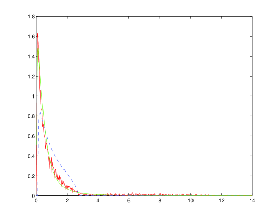
Figure 11: Comparison between the full spectral density from an ensemble generated using method 1 on set DJ ($48\times 20$ chopped ensemble). The generalised density eq. (2.7) fitted with $\alpha=1$, and the MP distribution eq. (2.2) are given by the full green line and dashed blue line, respectively.

Appendix B Consistency of Chopping in Method 2: Permutations

In this appendix we check the effect of taking different choppings in method 2 by comparing different ensembles when randomly permuting the rows (stocks) into different groups. We have created 10 different ensembles of the same size $48\times 20$ from data set SP. For each ensemble the 400 stocks were put into a different partition of 20 blocks of size 20.

The superposition of the smallest and second smallest eigenvalues from these 10 different ensembles generated by method 2 is shown in fig. 13. We find that both eigenvalues superimpose well to give a smoothed curve. For illustration we display the curves of the two eigenvalues averaged over these 10 ensembles in fig. 13 right, to illustrate their width and separation (compared to a single ensemble in fig. 6).

For curiosity we have done the same analysis for the largest and second largest eigenvalues within the same 10 ensembles as shown in fig. 14.

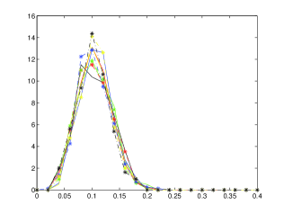
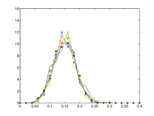
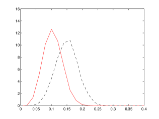
Figure 13: Consistency of the 2 smallest eigenvalues in method 2: 10 different choppings of the same size $48\times 20$ are obtained by using different partitions of the 400 stocks into 20 blocks of size 20: the overlapping of the smallest (left) and second smallest eigenvalue (middle) for these 10 different ensembles. Right plot: after taking the average over the 10 ensembles the averaged smallest (red left curve) and averaged second smallest eigenvalue (right dashed curve) are superimposed.

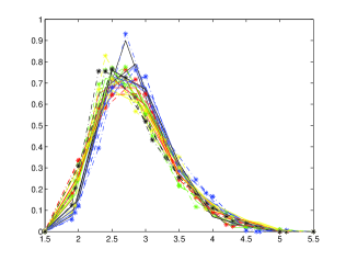
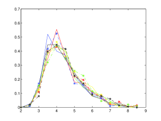
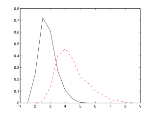
Figure 14: Consistency of the 2 largest eigenvalues in method 2 using the same method as in fig. 13: the overlapping the second largest (left) and largest eigenvalue (middle) from 10 different ensembles. Right plot: after taking the average over the 10 ensembles the averaged second largest (black left curve) and averaged largest eigenvalue (right dashed curve) are superimposed.

As we can see in fig. 14 the largest eigenvalues from the 10 different ensembles overlap smoothly. This fact makes its unlikely that in these ensembles the largest eigenvalues still represents the market movement as in [5, 6]. It would be very interesting to try to identify the largest eigenvalues in fig. 14 as a largest generalised TW eigenvalue from RMT as shown in fig 3 right. However, due to the lack of an analytic formula within our generalised RMT, and in particular because of the (possibly $\alpha$-dependent) scaling with $N$ this is a difficult task.

Appendix C Unfolding Routine

Consider the cumulative distribution of eigenvalues:

$$P(x)=N\int_{0}^{x}dx^{\prime}\rho(x^{\prime})$$ (C.1)

where $\rho(\lambda)$ is the smooth density of eigenvalues (normalised to $1$).

Given a set of $m$ samples of $N$ bare eigenvalues $\{\lambda_{1}^{(k)},\ldots,\lambda_{N}^{(k)}\}$ (with $k=1,\ldots,m$), we first define a set of unfolded eigenvalues $\{E_{1}^{(k)},\ldots,E_{N}^{(k)}\}$ as:

$$E_{j}^{(k)}=P(\lambda_{j}^{(k)})$$ (C.2)

Then the set of spacings $\{s\}$ to be histogrammed is computed by the nearest-neighbour difference among the $E$’s within each sample. Clearly, for empirical data the main problem is to estimate reliably the cumulative distribution $P(x)$. Given a regular grid of $K$ points $\{0\leq y_{1}\leq\ldots\leq y_{K}\}$ on the positive semi-axis, one can simply define an estimator $\tilde{P}(y_{r})$ for $P(x)$ as the number of bare eigenvalues (in total $mN$) falling below $y_{r}$, divided by $m$. This estimator approaches $N$ for large argument $y$. Then, in order to get a continuous distribution, one simply performs a polynomial fit of degree $d$ on the $\{y_{r},\tilde{P}(y_{r})\}$ pairs and approximates the true cumulative distribution with the fitting polynomial $p_{d}(x)\approx P(x)$.

The MATLAB code that performs the unfolding procedure as stated above and returns the positions $X$ of the bins and the normalised histogram $Y$ of the nearest neighbour spacings can be retrieved from the public domain web site [40].

References

- [1] M. Potters, J.P. Bouchaud, and L. Laloux, [arXiv:physics/0507111v1] (2005).
- [2] Z. Burda, J. Jurkiewicz and M.A. Nowak, Acta Physica Polonica B 34, 87 (2003).
- [3] D. Sornette, P. Simonetti, and J.V. Andersen, Physics Reports 335, 19 (2000).
- [4] L. Laloux, P. Cizeau, J.-P. Bouchaud, and M. Potters, Phys. Rev. Lett. 83, 1467 (1999).
- [5] V. Plerou, P. Gopikrishnan, B. Rosenow, L.A.N. Amaral, and H.E. Stanley, Phys. Rev. Lett. 83, 1471 (1999).
- [6] V. Plerou, P. Gopikrishnan, B. Rosenow, L.A.N. Amaral, T. Guhr, and H.E. Stanley, Phys. Rev. E 65, 066126 (2002).
- [7] F. Lillo and R.N. Mantegna, [cond-mat/0305546] (2003).
- [8] A. Utsugi, K. Ino, and M. Oshikawa, Phys. Rev. E 70, 026110 (2004); Y. Malevergne and D. Sornette, Physica A 331, 660 (2004).
- [9] S. Galluccio, J.-P. Bouchaud, and M. Potters, Physica A 259, 449 (1998).
- [10] Z. Burda, J. Jurkiewicz, M.A. Nowak, G. Papp, and I. Zahed, Acta Physica Polonica B 34, 4747 (2003).
- [11] Z. Burda, A. Jarosz, J. Jurkiewicz, M.A. Nowak, G. Papp, and I. Zahed, [arXiv:physics/0603024v1] (2006).
- [12] G. Biroli, J.-P. Bouchaud, and M. Potters, Acta Physica Polonica B 38, 4009 (2007).
- [13] G. Akemann and P. Vivo, J. Stat. Mech. P09002 (2008).
- [14] A.Y. Abul-Magd, G. Akemann, and P. Vivo, J. Phys. A: Math. Theor. 42, 175207 (2009).
- [15] M. Politi, E. Scalas, D. Fulger, and G. Germano, [arXiv:0903.1629] (2009).
- [16] J. Kwapień, S. Drożdż, A.Z. Gorski, and F. Oswiȩcimka, Acta Physica Polonica B 37, 3039 (2006).
- [17] C. Biely and S. Thurner, Quant. Fin. 8, 705 (2008); Acta Physica Polonica B 38, 4111 (2007).
- [18] T. Guhr and B. Kälber, J. Phys. A 36, 3009 (2003).
- [19] Z. Burda and J. Jurkiewicz, Physica A 344, 67 (2004).
- [20] J. Wishart, Biometrika 20, 32 (1928).
- [21] I.M. Johnstone, The Annals of Statistics 29, 295 (2001).
- [22] K. Johansson, Comm. Math. Phys. 209, 437 (2000); P. Vivo, S.N. Majumdar, and O. Bohigas, J. Phys. A: Math. Theor. 40, 4317 (2007); S.N. Majumdar, O. Bohigas, and A. Lakshminarayan, J. Stat. Phys. 131, 33 (2008).
- [23] E.V. Shuryak and J.J.M. Verbaarschot, Nucl. Phys. A 560, 306 (1993); J.J.M. Verbaarschot, Phys. Rev. Lett. 72, 2531 (1994); G. Akemann, P.H. Damgaard, U. Magnea and S. Nishigaki, Nucl. Phys. B 487, 721 (1997).
- [24] J. Ambjørn, C.F. Kristjansen, and Yu. Makeenko, Mod. Phys. Lett. A 7, 3187 (1992); G. Akemann, Nucl. Phys. B 507, 475 (1997); J. Ambjørn, Yu. Makeenko, and C.F. Kristjansen, Phys. Rev. D 50, 5193 (1994).
- [25] E. Telatar, Eur. Trans. Telecomm. 10, 585 (1999).
- [26] C.A. Tracy and H. Widom, Commun. Math. Phys. 159, 151 (1994); ibid. 177, 727 (1996).
- [27] O.N. Feldheim and S. Sodin, [arXiv:0812.1961v3] (2008).
- [28] Z. Burda, A. Görlich, and B. Wacław, Phys. Rev. E 74, 041129 (2006).
- [29] V.A. Marčenko and L.A. Pastur, Math. USSR-Sb 1, 457 (1967).
- [30] M. Müller, Y. López Jiménez, C. Rummel, G. Baier, A. Galka, U. Stephani, and H. Muhle, Phys. Rev. E 74, 041119 (2006).
- [31] S. Drożdż, J. Kwapień, and P. Oswiȩcimka, Acta Physica Polonica B 38, 4027 (2007).
- [32] F. Toscano, R.O. Vallejos, and C. Tsallis, Phys. Rev. E 69, 066131 (2004); A.C. Bertuola, O. Bohigas, and M.P. Pato, Phys. Rev. E 70, R065102 (2004); A.Y. Abul-Magd, Phys. Lett. A 333, 16 (2004).
- [33] A. Edelman and P.-O. Persson, [arXiv:math-ph/0501068v1] (2005).
- [34] G. Biroli, J.-P. Bouchaud, and M. Potters, [arXiv:cond-mat/0609070v1] (2006).
- [35] O. Bohigas, J.X. de Carvalho, and M.P. Pato Phys. Rev. E 79, 031117 (2009).
- [36] M.L. Mehta, Random Matrices, Academic Press, Third Edition, London (2004).
- [37] T. Guhr, A. Müller-Groeling, and H.A. Weidenmüller, Phys. Rep. 299, 190 (1998).
- [38] S. Jalan and J.N. Bandyopadhyay, Phys. Rev. E 76, 046107 (2007).
- [39] J.X. de Carvalho, S. Jalan, and M.S. Hussein, Phys. Rev. E 79, 056222 (2009).
- [40] http://www.mathworks.com/matlabcentral/fileexchange/24122 (2009).