Measurement of nonlinear frequency shift coefficient in spin-torque oscillators based on MgO tunnel junctions

Abstract

The nonlinear frequency shift coefficient, which represents the strength of the transformation of amplitude fluctuations into phase fluctuations of an oscillator, is measured for MgO-based spin-torque oscillators by analyzing the current dependence of the power spectrum. We have observed that linewidth against inverse normalized power plots show linear behavior below and above the oscillation threshold as predicted by the analytical theories for spin-torque oscillators. The magnitude of the coefficient is determined from the ratio of the linear slopes. Small magnitude of the coefficient ($\sim 3$) has been obtained for the device exhibiting narrow linewidth ($\sim 10~{}\mathrm{MHz}$) at high bias current.

Spin-torque oscillators (STOs) emit a microwave signal. The signal originates in magnetization oscillations excited by bias dc current in a magnetoresistive (MR) deviceKiselev ; Rippard . In recent years, extensive studies have been carried out on STOs because they are a promising candidate for an on-chip microwave oscillatorKatine ; Silva . One of the important properties of an STO is its frequency nonlinearity, i.e., a frequency depends on an oscillation amplitudeSlavin ; Rezende . Due to the property, the frequency of STO is tunable only by changing bias dc current, which is generally considered to be an advantage for applications. The nonlinearity is, however, a disadvantage of STO when thermal fluctuations are taken into account. According to the analytical theory of Kim et al.Kim , amplitude fluctuations are transformed into phase fluctuations because of the nonlinearity, resulting in spectrum linewidth broadening. The linewidth is a measure of the phase stability of oscillation and it is preferable that it be narrow. Estimating quantitatively the nonlinearity, which determines the device performances, is therefore a key subject for further developments of STOs. According to the recent theoriesKim ; Tiberkevich ; Kim2 ; Tiberkevich3 ; Kudo ; Slavin2 , the quantity representing the degree of the nonlinearity is the normalized dimensionless nonlinear frequency shift coefficient $\nu$ (regarding the definition of the coefficient, see, e.g., Eq. (7) of Ref. Tiberkevich3, or Eq. (9) of Ref. Kudo, ). In this letter, we report experimental estimations of the coefficient $\nu$ in MgO-based STOs near threshold, which have not been directly addressed by previous experiments. Following some theoretical remarks, experimental results are shown.

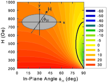
Figure 1: (Color online) Dependence of $\nu$ in the planar device with uniaxial anisotropy ($x$-direction) on the magnitude $H$ and the in-plane angle $\phi_{H}$ of in-plane external magnetic field. The parameters chosen are an uniaxial anisotropy field $H_{k}=200~{}\mathrm{Oe}$, a demagnetizing field $4\pi M_{\mathrm{s}}=8000~{}\mathrm{Oe}$, the Gilbert damping $\alpha_{\mathrm{G}}=0.01$, and the nonlinearity of dampingTiberkevich2 $q_{1}=3$. In the notation used here, positive and negative $\nu$ denotes the red and blue frequency shift, respectively.

It is theoretically known that the coefficient $\nu$ has various values depending on magnetic environments and dampingTiberkevich3 ; Kudo ; Slavin2 . In general, the coefficient $\nu$ also depends on bias current Tiberkevich3 ; Slavin2 . Considering that the variation of $\nu$ with bias current is small in the range near threshold, we treat $\nu$ as a constant independent of bias current.

First, we demonstrate numerically how large the coefficient $\nu$ is in typical STOs. A calculation example of $\nu$ at the threshold in a planar device with uniaxial anisotropy is shown in Fig. 1, representing the dependence on the magnitude and the angle of an in-plane external magnetic field. The calculation is performed by the method described in Ref. Kudo, which is based on the macrospin model. We have used the typical STO parameters shown in the figure caption. In the wide external field region, $|\nu|$ is much larger than unity ($|\nu|\sim 5$-$50$). On the black line shown in Fig. 1, the frequency nonlinearity vanishes (the nonlinearity due to the demagnetizing effect cancels out that due to the in-plane anisotropy), where remarkable reduction of linewidth is expectedSlavin2 ; Thadani ; Mizushima .

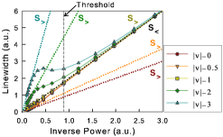
Figure 2: (Color online) Linewidth and inverse power near threshold for several values of $|\nu|$. The units of linewidth and power are appropriately scaled.

To estimate the value of $\nu$ from experiment, we have used the spectrum analysis method based on the theories of spectrum linewidth of STO under thermal fluctuations Kim ; Tiberkevich ; Kim2 ; Tiberkevich3 ; Kudo ; Slavin2 . The method is similar to the one often used to measure the linewidth enhancement factor ($\alpha$-factor) in lasersToffano97 . According to the theories, the linewidth shows asymptotic behavior below and above threshold. In the region below threshold (the thermal activated oscillation region), the linewidth is given by

$$\Delta f^{<}=\Delta f_{0}\times(k_{\mathrm{B}}T/E_{\mathrm{osci}}).$$ (1)

In the region above threshold (the current-induced oscillation region), the linewidth is given by

$$\Delta f^{>}=\Delta f_{0}\times(k_{\mathrm{B}}T/E_{\mathrm{osci}})\times(1+\nu^{2})/2,$$ (2)

in which the additional phase diffusion due to amplitude fluctuations is expressed by the factor of $\nu^{2}$. In Eqs. (1) and (2), $\Delta f_{0}$ is the damping at thermal equilibrium expressed in linewidth, $k_{\mathrm{B}}T$ is the thermal energy, and $E_{\mathrm{osci}}$ is the average magnetization oscillating energy of a certain oscillation mode. The energy $E_{\mathrm{osci}}$ becomes large as the bias current $I$ increases. Since the voltage oscillation signal from STO originates in the MR effect, $E_{\mathrm{osci}}$ is proportional to a ‘normalized’ power $P/I^{2}$, where $P$ is the power of voltage oscillation signal from STO. Therefore, Eqs. (1) and (2) both indicate that the linewidth is proportional to the inverse normalized power in the two asymptotic regions, i.e., $\Delta f^{<,>}\propto(P/I^{2})^{-1}$. Accordingly, drawing a linewidth versus inverse normalized power plot, we can extract $\nu$ from the following relation;

$$s_{>}/s_{<}=(1+\nu^{2})/2,$$ (3)

where $s_{<}$ and $s_{>}$ are the slopes of asymptotes below and above threshold, respectively. To visualize Eq. (3), we show the linewidth and inverse power calculated numerically in Fig. 2. The calculation is based on the Fokker-Planck equation (FPE) corresponding to a noisy nonlinear auto-oscillatorKim2 ; Seybold . We have used the single-Lorentzian approximation for a power spectrum. In the approximation, the linewidth is given by the real part of the first eigenvalue in the eigenmode expansion method for FPE ($\mathrm{Re}\Lambda_{1,1}$ in the notation of Ref. Kim2, ). In Fig. 2, linewidths show asymptotic behavior (dotted lines) represented by Eqs. (1) and (2) in the region below and above threshold, and the relation between the slopes of asymptotes (Eq. (3)) holds.

Measurements are performed on MgO-based planar magnetic tunnel junction devices at room temperature. Tunnel junctions are composed of IrMn(10)/PL/MgO(1.05)/FL, in which the free layer (FL) is a CoFeB(3) layer and the pinned layer (PL) is a CoFe(4)/Ru(0.95)/CoFeB(4) synthetic antiferromagnet trilayer. The junctions have been fabricated by sputter deposition with annealing for one hour in a high magnetic field and at the temperature of $300^{\circ}\mathrm{C}$. Nanopillar devices are patterned using electron-beam lithography and ion milling. On the same wafer, we find samples with various TMR ratio in the range $10$-$90\%$. We have observed that lower TMR ratio samples tend to show narrower spectral linewidth oscillations. This tendency in MgO-based samples is similar to that reported in Ref. Houssameddine08, . We consider that the difference of TMR ratio among samples may result from localized defects in the MgO barrier as speculated by the authors of Ref. Houssameddine08, . In this letter, we show the results of one typical low TMR ratio sample with a $200\times 120~{}\mathrm{nm}^{2}$ elliptical shape. From $R$-$H$ (resistance-field) characteristic measurements of the sample for several field angles, we find that the resistance is $235~{}\mathrm{\Omega}$ ($5.6~{}\mathrm{\Omega}\cdot\mathrm{\mu m}^{2}$) for parallel configuration, TMR ratio is $15.6~{}\%$, and an in-plane anisotropy field $H_{k}$ is about $200~{}\mathrm{Oe}$. The pinned layer magnetization is along the long axis of the ellipse without an applied field.

Oscillation properties are measured by a spectrum analyzer. We apply dc current $I$ to the sample with antiparallel magnetization configuration. Positive $I$ corresponds to electrons flowing from the pinned layer to the free layer. Oscillation properties vary sensitively with the field applied in the sample plane: the magnitude $H$ of $200$-$700~{}\mathrm{Oe}$ and the angle $\phi_{H}$ of $0$-$90^{\circ}$. When the angle $\phi_{H}\simeq 40^{\circ}\pm 5^{\circ}$ and the magnitude $H\simeq 500\pm 50~{}\mathrm{Oe}$, distinct oscillation peaks are observed. In the other applied fields, distinct peaks are not observed at any bias current ($I\leq 0.7~{}\mathrm{mA}$). Below, we show the results for the two setups of the applied fields in which narrow linewidths of $\sim 10~{}\mathrm{MHz}$ are observed: (I) $H=490~{}\mathrm{Oe}$ and $\phi_{H}=42.4^{\circ}$, and (II) $H=516~{}\mathrm{Oe}$ and $\phi_{H}=39.7^{\circ}$.

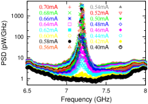
Figure 3: (Color online) PSD of the voltage oscillation signal in the setup (I) for bias currents from $0.4$ to $0.7~{}\mathrm{mA}$.

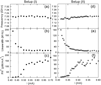
Figure 4: Frequency ((a) and (d)), FWHM linewidth $\Delta f$ ((b) and (e)), and normalized power $P/I^{2}$ ((c) and (f)) vs. bias current $I$ for the setups (I) and (II). In (b), $\Delta f\simeq 14~{}\mathrm{MHz}$ at $0.58~{}\mathrm{mA}$. In (e), $\Delta f\simeq 8.6~{}\mathrm{MHz}$ at $0.56~{}\mathrm{mA}$.

Power spectral density (PSD) of the voltage oscillation signal in the setup (I) is shown in Fig. 3. The characteristic oscillation mode is observed around $7.2~{}\mathrm{GHz}$ for the bias current $I\geq 0.42~{}\mathrm{mA}$. This mode grows steeply as the bias current increases and exhibits narrow linewidth in the high-current region. The PSD in the setup (II) is similar to that in the setup (I). The dependence of the frequency, the full width at half maximum (FWHM) linewidth, and the normalized power of the mode on the bias current for the setups (I) and (II) is shown in Fig. 4. The data are obtained by Lorentzian fits to the spectral peaks of the characteristic oscillation modes. The broken lines in Fig. 4 denote the threshold currents $I_{\mathrm{th}}$. The normalized power below threshold depends on the bias current in the way that $(P/I^{2})^{-1}\propto(I_{\mathrm{th}}-I)$.Tiberkevich By using the expression, we find that $I_{\mathrm{th}}\simeq 0.46~{}\mathrm{mA}$ for the setup (I) and $I_{\mathrm{th}}\simeq 0.44~{}\mathrm{mA}$ for the setup (II). In Figs. 4 (a) and (d), the frequency shift with the bias current is much smaller than that observed in previous experiments for MgO-based STOsHoussameddine08 ; Georges , and we cannot judge whether the shift is red or blue. In Figs. 4 (c) and (f), the normalized power grows steeply up to the current $I\simeq 0.52~{}\mathrm{mA}$ from the threshold current. For $I>0.52~{}\mathrm{mA}$, the normalized power is being saturated.

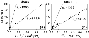
Figure 5: (a) and (b) $\Delta f$ vs. $(P/I^{2})^{-1}$-plots for the setups (I) and (II).

From the data for linewidth $\Delta f$ and normalized power $P/I^{2}$ shown in Figs. 4, we have obtained the $\Delta f$ vs. $(P/I^{2})^{-1}$-plots shown in Figs. 5. We have used the data for the current $I\leq 0.52~{}\mathrm{mA}$. As predicted by the theories, we observe that linewidth against inverse normalized power plots show linear behavior below and above the threshold. The appearance of the linear behavior above the threshold supports the consideration that the variation of $\nu$ with bias current is small in the range near threshold. By estimating the values of linear slopes $s_{<,>}$ and using Eq. (3), we find the coefficient $|\nu|\simeq 2.9$ for the setup (I) and $|\nu|\simeq 2.6$ for the setup (II). Considering the range of values expected by the calculation as shown in Fig. 1, these values of the coefficient ($|\nu|\sim 3$) are comparatively small. The smallness is consistent with the flatness of frequency (Figs. 4 (a) and (d)) and the exhibition of narrow linewidths of $\sim 10~{}\mathrm{MHz}$ in the high-current region (Figs. 4 (b) and (e)). According to Fig. 1, the coefficient $|\nu|$ is expected to have small values when an in-plane field is applied to the hard axis, i.e., $\phi_{H}\sim 80$-$90^{\circ}$. Our results measured in the angle of $\phi_{H}\sim 40^{\circ}$ are inconsistent with the expectation. We consider that the mode with $7.2~{}\mathrm{GHz}$ peak may be a non-uniform mode and so the effective directions and structures of in-plane anisotropy for the magnetization composing the mode are complicated. Micromagnetic study to clarify the oscillation mode is now in progress.

In summary, we estimated the coefficient $\nu$ in MgO-based STOs which is a measure of the transformation of amplitude fluctuations into phase fluctuations of an oscillator. For the device exhibiting narrow linewidth ($\Delta f\sim 10~{}\mathrm{MHz}$) in a high-current region, small value of the coefficient ($|\nu|\sim 3$) was obtained.

References

- (1) S. I. Kiselev, J. C. Sankey, I. N. Krivorotov, N. C. Emley, A. G. F. Garcia, R. J. Schoelkopt, R. A. Buhrman, and D. C. Ralph, Nature 425, 380 (2003).
- (2) W. H. Rippard, M. R. Pufall, S. Kaka, T. J. Silva, and S. E. Russek, Phys. Rev. Lett. 92, 027201 (2004).
- (3) J. A. Katine and E. E. Fullerton, J. Magn. Magn. Mater. 320, 1217 (2008).
- (4) T. J. Silva and W. H. Rippard, J. Magn. Magn. Mater. 320, 1260 (2008).
- (5) A. N. Slavin and P. Kabos, IEEE Trans. Magn. 41, 1264 (2005).
- (6) S. M. Rezende, F. M. de Aguiar, and A. Azevedo, Phys. Rev. Lett. 94, 037202 (2005).
- (7) J.-V. Kim, V. Tiberkevich, and A. N. Slavin, Phys. Rev. Lett. 100, 017207 (2008).
- (8) V. Tiberkevich, A. N. Slavin, and J.-V. Kim, Appl. Phys. Lett. 91, 192506 (2007).
- (9) J.-V. Kim, Q. Mistral, C. Chappert, V. S. Tiberkevich, and A. N. Slavin, Phys. Rev. Lett. 100, 167201 (2008).
- (10) V. Tiberkevich, A. N. Slavin, and J.-V. Kim, Phys. Rev. B 78, 092401 (2008).
- (11) K. Kudo, T. Nagasawa, R. Sato, and K. Mizushima, J. Appl. Phys. 105, 07D105 (2009).
- (12) A. N. Slavin and V. Tiberkevich, IEEE Trans. Magn. 45, 1875 (2009).
- (13) V. Tiberkevich and A. Slavin, Phys. Rev. B 75, 014440 (2007).
- (14) K. V. Thadani, G. Finocchio, Z.-P. Li, O. Ozatay, J. C. Sankey, I. N. Krivorotov, Y.-T. Cui, R. A. Buhrman, and D. C. Ralph, Phys. Rev. B 78, 024409 (2008).
- (15) K. Mizushima, T. Nagasawa, K. Kudo, Y. Saito, and R. Sato, Appl. Phys. Lett. 94, 152501 (2009).
- (16) Z. Toffano, IEEE J. Sel. Topics Quantum Electron. 3, 485 (1997).
- (17) K. Seybold and H. Risken, Z. Physik 267, 323 (1974).
- (18) D. Houssameddine, S. H. Florez, J. A. Katine, J.-P. Michel, U. Ebels, D. Mauri, O. Ozatay, B. Delaet, B. Viala, L. Folks, B. D. Terris, and M.-C. Cyrille, Appl. Phys. Lett. 93, 022505 (2008).
- (19) B. Georges, J. Grollier, V. Cros, A. Fert, A. Fukushima, H. Kubota, K. Yakushijin, S. Yuasa, and K. Ando, arXiv:0904.0880v1.