$\alpha_{s}$ from $\tau$ decays: contour-improved versus fixed-order summation in a new QCD perturbation expansion

Abstract

We consider the determination of $\alpha_{s}$ from $\tau$ hadronic decays, by investigating the contour-improved (CI) and the fixed-order (FO) renormalization group summations in the frame of a new perturbation expansion of QCD, which incorporates in a systematic way the available information about the divergent character of the series. The new expansion functions, which replace the powers of the coupling, are defined by the analytic continuation in the Borel complex plane, achieved through an optimal conformal mapping. Using a physical model recently discussed by Beneke and Jamin, we show that the new CIPT approaches the true results with great precision when the perturbative order is increased, while the new FOPT gives a less accurate description in the regions where the imaginary logarithms present in the expansion of the running coupling are large. With the new expansions, the discrepancy of 0.024 in $\alpha_{s}(m_{\tau}^{2})$ between the standard CI and FO summations is reduced to only 0.009. From the new CIPT we predict $\alpha_{s}(m_{\tau}^{2})=0.320\,\,^{+0.011}_{-0.009}$, which practically coincides with the result of the standard FOPT, but has a more solid theoretical basis.

1 Introduction

The precise determination of $\alpha_{s}$ from $\tau$ hadronic decays is one of the most important results in perturbative QCD PDG2008 . The subject has been treated by many authors (see Bra88 -Maltman08 and references therein). Among the most important improvements we mention the so-called ”contour-improved renormalization-group summation” Pivo , DiPi , which avoids the large logarithms of the usual ”fixed-order” expansion along the integration contour relevant for $\alpha_{s}$ extraction. The higher orders of perturbation theory, expressed by the so-called renormalons, were also investigated, especially as concerns their effect on the precision of the theoretical determinations BBB , Neub .

The problem was revisited recently, after the calculation of the Adler function up to fourth order BCK08 , the same at which the $\beta$ function describing the running of the coupling is known LaRi , Czakon . The determination of $\alpha_{s}$ from the ALEPH spectral function data was reconsidered in Davier2008 , where the prediction based on CIPT $\alpha_{s}(m_{\tau}^{2})=0.344\pm 0.009$ was made. On the other hand, an updated version of FOPT BeJa led to the prediction $\alpha_{s}(m_{\tau}^{2})=0.320^{+0.012}_{-0.007}$. As remarked in BeJa , the discrepancy of 0.024 between CIPT and FOPT appears to be the largest systematic theoretical uncertainty in the $\alpha_{s}$ determination, and it does not go away by adding the presently known higher-order terms.

The two summation methods were analyzed in detail in BeJa by means of a ”physical” model for the Borel transform of the Adler function. The conclusion of this study was that, somewhat surprisingly, FOPT is preferable, CIPT failing to approach the true result, although it is a priori more consistent.

The purpose of the present work is to understand better the relation between the CI and FO summation methods and their consequences on the extraction of $\alpha_{s}$. To this end we investigate these two methods using a new perturbation expansion advocated by us some time ago CaFi . The new expansion separates the intrinsic ambiguity of the perturbation theory due to the infrared regions of the Feynman diagrams, from the divergent character of the series. This is achieved if the usual perturbative expansion is replaced by a series with better convergence properties (each new term improving the accuracy of the approximation instead of spoiling it). As shown in CaFi -CaFi2 , the new expansion is defined by using the analytic continuation in the Borel complex plane by an optimal conformal mapping. The properties of the novel expansion functions were analyzed in detail in CaFi1 ,CaFi2 and some applications were discussed in CaFi , ChFi .

The paper is organized as follows: in Section 2 we briefly review the CI and FO summations of the Adler function relevant for $\tau$ decays. In Section 3 we discuss the Borel transform and in Section 4 we present the CI and FO versions of the new perturbation theory for the Adler function. In Section 5 we apply these two methods to calculate $\alpha_{s}(m_{\tau}^{2})$, and show that the difference between the two predictions is significantly smaller than in the standard case. In order to understand these results, in Section 6 we investigate the new expansions using as an example the physical model proposed in BeJa . More comments on the method of conformal mapping and its relevance for the physical case are made in Section 7. We summarize our results in Section 8, where we emphasize that the CI summation combined with the new perturbation expansion leads to a precise determination of $\alpha_{s}(m_{\tau}^{2})$.

2 Standard CIPT and FOPT

The relevant quantity for the extraction of $\alpha_{s}(m_{\tau}^{2})$ is the integral

$$\delta^{(0)}=\frac{1}{2\pi i}\,\oint\limits_{|s|=s_{0}}\,\frac{ds}{s}\,\omega(s)\,\hat{D}(s)\,,$$ (1)

where $s_{0}=m_{\tau}^{2}$, $\omega(s)=1-2s/s_{0}+2(s/s_{0})^{3}-(s/s_{0})^{4}$ and $\hat{D}(s)=D(s)-1$ is the reduced Adler function in massless QCD. It is written formally as the renormalization-group improved series

$$\hat{D}(s)=\sum_{n=1}^{\infty}K_{n}\,(a_{s}(s))^{n}\,,$$ (2)

where $a_{s}(s)\equiv\alpha_{s}(s)/\pi$. In the $\overline{MS}$ scheme, for $n_{f}=3$, the coefficients $K_{n}$ calculated up to now have the values:

$$K_{1}=1,~{}~{}K_{2}=1.6398,~{}~{}K_{3}=6.3712,~{}~{}K_{4}=49.076.$$ (3)

Several methods were proposed for estimating the higher-order perturbative coefficients from the low-order ones KaSt , BCK03 . In particular, in BeJa the authors adopt the value

$$K_{5}=283.$$ (4)

We mention that at large $n$ the coefficients display a factorial increase, $K_{n}\sim n!$, so that the series in (2) is divergent. In writing (2) we follow the convention often adopted in physical papers, writing the sign of equality even if the series on the right hand side is divergent and the equality is impossible. According to Dyson’s proposal Dyson from 1952, the series is then regarded as asymptotic to $\hat{D}(s)$ standing on the left hand side. If the series is convergent, the relation (2) is understood as equality. Analogous series in the text below (see (16), (20), (27), (30), etc.) are understood in a similar sense.

The contour-improved (CI) summation amounts to introducing (2) in (1), and performing the integral with $a_{s}(s)$ calculated locally from the solution of the renormalization group equation. The solution is known at present up to four loops LaRi , the first coefficients $\beta_{j}$ of the $\beta$ function, calculated in the $\overline{MS}$ scheme and $n_{f}=3$ being

$$\beta_{0}=9/4,~{}~{}\beta_{1}=4,~{}~{}\beta_{2}=10.0599,~{}~{}\beta_{3}=47.228.$$ (5)

The Taylor expansion of $a_{s}(s)$ in terms of a reference point $s_{1}$ reads

$$a_{s}(s)=\sum\limits_{j\geq 1}\,\xi_{j}\,(a_{s}(s_{1}))^{j},$$ (6)

where the coefficients $\xi_{j}$ depend on $\eta_{1}=\ln(s/s_{1})$ and on the coefficients $\beta_{j}$. By inserting this expansion with $s_{1}=s_{0}$ in (2) and rearranging the expansion in powers of $a_{s}(s_{0})$, one obtains the FO summation, which can be written as

$$\hat{D}(s)=\sum_{n=1}^{\infty}[K_{n}+\kappa_{n}(s)]\,(a_{s}(s_{0}))^{n}\,,$$ (7)

where $\kappa_{n}(s)$ are polynomials of $\eta_{0}=\ln(s/s_{0})$, and depend on the coefficients $\beta_{j}$ and $K_{j}$ for $j\leq n$.

3 Borel transform

The series (2) can be formally written as the Borel-Laplace transform

$$\hat{D}(s)=\frac{1}{\beta_{0}}\,\int\limits_{0}^{\infty}\!{\rm e}^{-u/(\beta_{0}a_{s}(s))}\,B(u)\,{\rm d}u\,,$$ (8)

where $B(u)$ is the Borel transform of the Adler function, defined by the power series

$$B(u)=\sum\limits_{n=0}^{\infty}b_{n}u^{n}\,,$$ (9)

with $b_{n}$ related to the original perturbative coefficients appearing in (2) by

$$b_{n}=\frac{K_{n+1}}{\beta_{0}^{n}\,n!}\,,\quad n\geq 0.$$ (10)

According to present knowledge, the function $B(u)$ has branch point singularities in the $u$-plane, along the negative axis - the ultraviolet (UV) renormalons - and the positive axis - the infrared (IR) renormalons Beneke . Specifically, the branch cuts are situated along the rays $u\leq-1$ and $u\geq 2$. The nature of the first branch points was established in Muel and in BBK (see also BeJa ). Thus, near the first branch points, i.e. for $u\sim-1$ and $u\sim 2$, respectively, $B(u)$ behaves as

$$B(u)\sim\frac{r_{1}}{(1+u)^{\gamma_{1}}},\quad B(u)\sim\frac{r_{2}}{(1-u/2)^{\gamma_{2}}},$$ (11)

where the residues $r_{1}$ and $r_{2}$ are not known, but the exponents $\gamma_{1}$ and $\gamma_{2}$ are known Muel , BBK .

Due to the singularities along the positive axis, the integral (8) does not exist. The ambiguity in the choice of prescription is often used as a measure of the uncertainty of the calculations in perturbative QCD. It is convenient to define the integral by the Principal Value (PV) prescription:

$$\hat{D}(s)\equiv\frac{1}{\beta_{0}}\,{\rm PV}\int\limits_{0}^{\infty}\!{\rm e}^{-u/(\beta_{0}a_{s}(s))}\,B(u)\,{\rm d}u\,,$$ (12)

where

$${\rm PV}\int\limits_{0}^{\infty}f(u){\rm d}u\equiv\frac{1}{2}\int\limits_{0}^{\infty}\left[f(u+i\epsilon){\rm d}u+f(u-i\epsilon){\rm d}u\right],~{}~{}\epsilon\to 0.$$

As discussed in CaNe , CaFi3 , the PV prescription is the best choice if one wants to preserve as much as possible the analyticity properties of the correlators in the $s$-plane, which are connected with causality and unitarity.

4 New CIPT and FOPT

In order to define a new perturbative expansion of the Adler function we shall apply the method of conformal mapping CiFi . This method is not applicable to the series (2), because ${\hat{D}}(s)$ (regarded as a function of $a_{s}(s)$) is singular at the point of expansion $a_{s}(s)=0$. The method can, on the other hand, be applied to (9), because $B(u)$ is holomorphic at $u=0$.

We note that the expansion (9) converges only in the disk $|u|<1$. A series with a larger domain of convergence can be obtained by expanding $B(u)$ in powers of a new variable. As shown in CiFi , the optimal variable coincides with the function that performs the conformal mapping of the whole analyticity domain of the expanded function onto a disk in the new complex plane.

To find the explicit form of the optimal conformal mapping, one should know the location of all the singularities of the Borel transform $B(u)$ in the complex Borel plane. Unfortunately, present evidence of these singularities is scarce: the known singularities (IR and UV renormalons and instanton-antiinstanton pairs) are produced only by a subclass of Feynman diagrams, while the effect of all the diagrams on the nature and location the singularities is not known. In the lack of rigorous results, additional assumptions are made or special models are built. As for additional assumptions, we point out that universally adopted has been to assume that $B(u)$ has only the above-mentioned singularities on the real axis with a gap, being holomorphic elsewhere.

Under this assumption, the optimal variable defined in CiFi reads CaFi :

$$w(u)=\frac{\sqrt{1+u}-\sqrt{1-u/2}}{\sqrt{1+u}+\sqrt{1-u/2}}.$$ (13)

This function maps the $u$-plane cut for $u\geq 2$ and $u\leq-1$ onto the unit disk $|w|<1$ in the complex plane $w=w(u)$, such that $w(0)=0$, $w(2)=1$ and $w(-1)=-1$. It is useful to give also the inverse $u=u(w)$ of (13):

$$u(w)=\frac{8w}{3-2w+3w^{2}}.$$ (14)

According to general arguments CiFi , the expansion

$$B(u)=\sum_{n\geq 0}d_{n}\,w^{n}$$ (15)

converges in the whole disk $|w|<1$. Moreover, as shown in CiFi , the expansion (15) has the best asymptotic rate of convergence compared to all the expansions of the function $B(u)$ in powers of other variables.

The series (15) can be used to define an alternative expansion of $\hat{D}(s)$. This is obtained formally by inserting (15) into (12) and interchanging the order of summation and integration. Thus, we adopt the modified CIPT expansion defined as CaFi -CaFi2

$$\hat{D}(s)=\sum\limits_{n\geq 0}d_{n}W_{n}(s),$$ (16)

where

$$W_{n}(s)=\frac{1}{\beta_{0}}{\rm PV}\int\limits_{0}^{\infty}\!{\rm e}^{-u/(\beta_{0}a_{s}(s))}\,w^{n}\,{\rm d}u\,.$$ (17)

We empahsize that the expansion (15) exploits only the location of the singularities in the Borel plane. However, in our case some information exists also about the nature of the singularities. We note that Eq. (11) expressed in the variable $w=w(u)$ implies

$$B(u)\sim\frac{(8/3)^{\gamma_{1}}r_{1}}{(1+w)^{2\gamma_{1}}},\quad\quad B(u)\sim\frac{(4/3)^{\gamma_{2}}r_{2}}{(1-w)^{2\gamma_{2}}},$$ (18)

for the behaviour near the points $w=-1$ and $w=1$, respectively. The expansion (15) is expected to describe these singularities if a large number of terms is used. However, since the nature of the singularities is known, it is convenient to incorporate it explicitly. This is achieved, for instance, by expanding the product $(1+w)^{2\gamma_{1}}(1-w)^{2\gamma_{2}}\,B(u)$ in powers of the variable $w$:

$$(1+w)^{2\gamma_{1}}(1-w)^{2\gamma_{2}}B(u)=\sum\limits_{n\geq 0}c_{n}\,w^{n}.$$ (19)

The expansion (19) converges in the whole disk $|w|<1$, i.e. in the whole complex $u$-plane, up to the cuts along the real axis. Moreover, since the singular behaviour of $B(u)$ at the first branch points is compensated by the first factors in (19), the series is expected to converge faster than (15). Also, the behaviour near the first singularities holds even for truncated expansions, which are used in practice.

It is important to stress that, while the expansion (15) is unique, the explicit inclusion of the first singularities of $B(u)$ contains some arbitrariness. The description of the singularities by multiplicative factors is a possibility, but is not a priori necessary. Moreover, the factors are not unique. For instance, the information on the nature of the singularities can be exploited by factors in the $u$ variable. An advantage of the choice (19) is that the multiplicative factors remain finite at large $u$. We will make more comments on this in Section 7.

The expansion (19) suggests the definition of the new CIPT

$$\hat{D}(s)=\sum\limits_{n\geq 0}c_{n}{\cal W}_{n}(s),$$ (20)

where the expansion functions are defined as

$${\cal W}_{n}(s)=\frac{1}{\beta_{0}}{\rm PV}\int\limits_{0}^{\infty}\!{\rm e}^{-u/(\beta_{0}a_{s}(s))}\,\frac{w^{n}}{(1+w)^{2\gamma_{1}}(1-w)^{2\gamma_{2}}}\,{\rm d}u\,,$$ (21)

with $w=w(u)$ defined in (13).

We emphasize that the expansions (16) and (20) reproduce the coefficients $K_{n}$ of the usual expansion (2), when the functions (17) and (21) are expanded in powers of the coupling. In fact, as shown in CaFi2 , the new expansion functions are formally represented by divergent series in powers of the coupling, much like the expanded correlator itself.

To obtain the FO version of the new expansions, we start from (7) and define the corresponding Borel transform

$$\tilde{B}(u,s)=\sum\limits_{n=0}^{\infty}\tilde{b}_{n}(s)u^{n}\,,$$ (22)

where

$$\tilde{b}_{n}(s)=\frac{K_{n+1}+\kappa_{n+1}(s)}{\beta_{0}^{n}\,n!}\,,\quad n\geq 0.$$ (23)

Then the Adler function admits the formal representation

$$\hat{D}(s)=\frac{1}{\beta_{0}}\,\int\limits_{0}^{\infty}\!{\rm e}^{-u/(\beta_{0}a_{s}(s_{0}))}\,\tilde{B}(u,s)\,{\rm d}u\,.$$ (24)

By comparing Eqs.(22), (23) with (9), (10), we can write

$$\tilde{B}(u,s)=B(u)+B_{1}(u,s),$$ (25)

where $B_{1}(u,s)$ is generated by the second term in the coefficients (23). It follows that the singularities of $B(u)$ are present also in the function $\tilde{B}(u,s)$, which may have in addition singularities from the second term in (25). In what follows we shall exploit the singularities of $B(u)$, which are known, by expanding $\tilde{B}(u,s)$ in powers of the variable $w$ defined above:

$$\tilde{B}(u,s)=\sum\limits_{n\geq 0}\tilde{d}_{n}(s)\,w^{n}.$$ (26)

This leads us to the definition of a modified FOPT, analogous to the CIPT expansion (16):

$$\hat{D}(s)=\sum\limits_{n\geq 0}\tilde{d}_{n}(s)\,\tilde{W}_{n},$$ (27)

in terms of the functions

$$\tilde{W}_{n}=\frac{1}{\beta_{0}}{\rm PV}\int\limits_{0}^{\infty}\!{\rm e}^{-u/(\beta_{0}a_{s}(s_{0}))}\,w^{n}\,{\rm d}u\,.$$ (28)

As we discussed above, it is convenient to impose explicitly the behaviour (11), which is done by expanding

$$(1+w)^{2\gamma_{1}}(1-w)^{2\gamma_{2}}\tilde{B}(u,s)=\sum\limits_{n\geq 0}\tilde{c}_{n}(s)\,w^{n}.$$ (29)

Then, using (24) we define the new FO expansion:

$$\hat{D}(s)=\sum\limits_{n\geq 0}\tilde{c}_{n}(s)\,\tilde{\cal W}_{n},$$ (30)

in terms of the functions

$$\tilde{\cal W}_{n}=\frac{1}{\beta_{0}}{\rm PV}\int\limits_{0}^{\infty}\!{\rm e}^{-u/(\beta_{0}a_{s}(s_{0}))}\,\frac{w^{n}}{(1+w)^{2\gamma_{1}}(1-w)^{2\gamma_{2}}}\,{\rm d}u\,.$$ (31)

In the next Section we shall determine $\alpha_{s}$ using the new CI and FO perturbation expansions (20), (21) and (30), (31), which include in an explicit way the nature of the first singularities of the Borel transform. More comments on them and the general expansions (16), (17) and (27), (28), which replace the standard CIPT and FOPT, respectively, will be made in Section 7.

By inserting (20) in the integral (1), with $a_{s}(s)$ calculated from RGE applied locally, we obtain a new CI perturbation expansion for $\delta^{(0)}$. Likewise, by using in the integral (1) the expansion (30), we obtain the new FO perturbation expansion of $\delta^{(0)}$.

We end this Section with a comment about the renormalization scale. The starting point of our derivation was the renormalization group improved expansion (2), which corresponds to the choice of the scale $\xi=1$ (with the notation used in Davier2008 ). The general case

$$\hat{D}(s)=\sum_{n=1}^{\infty}\hat{K}_{n}(\xi)\,(a_{s}(\xi s))^{n}\,,$$ (32)

with the coefficients $\hat{K}_{n}(\xi)$ given in Davier2006 , is easily obtained by reordering (2) as a series in powers of $a_{s}(\xi s)$. Similarly, the more general version of the FOPT

$$\hat{D}(s)=\sum_{n=1}^{\infty}[\hat{K}_{n}(\xi)+\hat{\kappa}(s,\xi)]\,(a_{s}(\xi s_{0}))^{n}\,,$$ (33)

is obtained by reordering (32) in powers of $a_{s}(\xi s_{0})$.

Starting from (32) and (33), the new CI and FO expansions for an arbitrary scale can be obtained in a straightforward way. Both the expansion coefficients and the expansion functions appearing in the generalizations of (20) and (30) will depend on the scale $\xi$.

5 Determination of $\alpha_{s}(m_{\tau}^{2})$

Our objective is to compare the results of the standard CIPT and FOPT from Davier2008 , BeJa , with the predictions of the new perturbation expansion presented in Section 4. To facilitate the comparison, we shall adopt the phenomenological value quoted in BeJa :

$$\delta^{(0)}_{\rm phen}=0.2042\pm 0.0050.$$ (34)

The determination of $\alpha_{s}(m_{\tau}^{2})$ then amounts to the calculation of $\delta^{(0)}$ defined in (1) using a specific expansion of $\hat{D}(s)$ for $s_{0}=m_{\tau}^{2}$, and solving the equation $\delta^{(0)}=\delta^{(0)}_{\rm phen}$ with respect to the coupling.

We use the known coefficients $K_{n}$ from (3). For $K_{5}$ we adopt the central value (4) with an error of $\pm$ 50%. Moreover, we follow the analysis made in BeJa , based on earlier works Muel , BBK , Beneke , which leads to:

$$\gamma_{1}=1.21,\quad\quad\gamma_{2}=2.58.$$ (35)

The Taylor coefficients $b_{n}$ of the Borel transform, defined in (10), are

$$b_{0}=1,\quad b_{1}=0.7288,\quad b_{2}=0.6292$$

$$b_{3}=0.7181,\quad b_{4}=0.4601.$$ (36)

Then the coefficients $c_{n}$ appearing in the new expansion (19), truncated at $n\leq 4$ read:

$$c_{0}=1,\quad c_{1}=-0.7973,\quad c_{2}=0.4095,$$ (37)

$$c_{3}=8.6647,\quad c_{4}=2.2416.$$

The new CIPT is given by the expansion (20) truncated after $N=5$ terms, with the numerical values of $c_{n}$ given in (37) and the functions ${\cal W}_{n}(s)$ defined in (21). Inserting (20) into (1) and using (34), we obtain the prediction of the new CIPT:

$$\alpha_{s}(m_{\tau}^{2})=0.3198\pm 0.0042_{\rm exp}\,^{+0.0099}{}_{-0.0076}\,{}_{\rm K_{5}}\,^{+0.0015}{}_{-0.0019}\,{}_{\rm scale},$$ (38)

where the experimental error is due to the uncertainty quoted in (34), the second error is obtained by varying the coefficient $K_{5}$ given in (4) by $\pm$ 50%, and the last error is obtained by varying the scale $\xi$ between $1-0.63$ and $1+0.63$ Davier2008 .

For the new FOPT the coefficients $\tilde{c}_{n}(s)$ defined in (29) as:

$$\tilde{c}_{0}(s)=1,$$

$$\tilde{c}_{1}(s)=-0.7973-2.6667\,\eta_{0},$$

$$\tilde{c}_{2}(s)=0.4095-2.4610\,\eta_{0}+3.5556\,\eta_{0}^{2},$$

$$\tilde{c}_{3}(s)=8.6647-0.6704\,\eta_{0}+8.1489\,\eta_{0}^{2}-3.1605\,\eta_{0}^{3},$$

$$\tilde{c}_{4}(s)=2.2416-18.1308\,\eta_{0}+6.7302\,\eta_{0}^{2}-11.0153\,\eta_{0}^{3},$$

$$~{}~{}~{}~{}+2.107\,\eta_{0}^{4},$$ (39)

where $\eta_{0}=\ln(s/s_{0})$.

The new FOPT is given by the expansion (30) truncated after 5 terms, with the numerical values of $\tilde{c}_{n}(s)$ given in (5) and $\tilde{\cal W}_{n}$ defined in (31). Inserting (30) into (1) and using (34), we obtain the prediction from the new FOPT:

$$\alpha_{s}(m_{\tau}^{2})=0.3113\pm 0.0038_{\rm exp}\,\pm 0.0013_{\rm K_{5}}\,^{+0.0103}{}_{-0.0006}\,{}_{\rm scale},$$ (40)

where the errors have the same significance as in (38).

As seen from (38) and (40), CIPT is more sensitive to the uncertainty of the last perturbative term, while FOPT is sensitive to the ambiguity of the renormalization scale. This is similar to what is obtained with the standard summations Davier2008 .

Before discussing in more detail these predictions, it is useful to investigate the new expansions given in Section 4 in the case of a physical model for the Adler function BeJa .

6 Model of Beneke and Jamin

The physical model proposed in BeJa is a parametrization of the Borel transform $B(u)$, consisting of one UV renormalon and two IR renormalons with specified branch point behaviour, multiplied by polynomials. The parameters of the model were adjusted such as to reproduce the first five coefficients $K_{n}$ given in Eqs. (3) and (4). The explicit expressions and the values of the parameters are given in Section 6 of BeJa , and we shall not reproduce them here.

The new CIPT and FOPT can be constructed in a staightforward way: from the parameters $K_{n}$ of the model one computes the Borel function (9) truncated after a certain number of terms $N$. The coefficients $c_{n}$ and $\tilde{c}_{n}(s)$ at that order are calculated from the expansions (19) and (29), respectively. The new expansions are given by (20) and (30), truncated at the same number of terms $N$, the expansion functions being defined in (21) and (31), respectively.

As in BeJa , we assume that the expansion of the $\beta$ function contains only four terms, with the coefficients given by (5). For $\alpha_{s}(m_{\tau}^{2})=0.34$ the exact value of $\delta^{(0)}$, obtained with the PV of the Borel sum, Eq. (12), is BeJa

$$\delta^{(0)}_{BS}=0.2371\pm 0.0060\,i,$$ (41)

where the error is an estimate of the prescription ambiguity (cf. Eq. (6.3) of BeJa ). We note that the ”exact” results are obtained by using the contour improved Borel sum (8), with $B(u)$ of the form specified by the model.

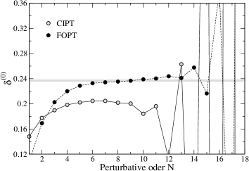
Figure 1: Values of $\delta^{(0)}$ for the model of Beneke and Jamin calculated with the standard CIPT and FOPT, as a function of the order up to which the series have been summed. The horizontal band is the exact value (41).

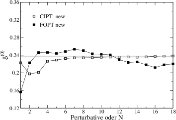
Figure 2: Values of $\delta^{(0)}$ for the model of Beneke and Jamin, calculated with the new CIPT and FOPT defined by Eqs. (20) and (30), respectively, as a function of the perturbative order $N$. The horizontal band is the exact value (41).

The comparison of the standard CIPT and FOPT with the new CIPT and FOPT is seen from Figs. 1 and 2, where we show $\delta^{(0)}$ calculated as a function of the order up to which the series have been summed. Fig. 1 reproduces Fig. 7 of BeJa , and shows that the standard CIPT does not approach the true value, staying below it up to the orders at which the results start to exhibit large oscillations. On the contrary, as seen in Fig. 2, the new CIPT gives very good results which approach the true value with great accuracy when $N$ increases. As concerns FOPT, the new approach gives results somewhat poorer than the standard one at low orders. At large orders, when the standard FOPT shows large oscillations, the new FOPT leads to values closer to the true result, but not as good as those obtained with the new CIPT.

In order to understand the origin of these results, we calculated the Adler function $\hat{D}(s)$ for complex $s$ along the integration contour. In Figs. 3 - 6 we present the real part of $\hat{D}(s)$ calculated with the standard/new CIPT and FOPT, for $s$ along the upper semicircle in the definition (1) of $\delta^{(0)}$ ($s=m_{\tau}^{2}\rm{e}^{i\varphi}$, for $0\leq\varphi\leq\pi$). Figs. 3 and 5 reproduce Fig. 9 of BeJa . In Figs. 7 - 10 we present the imaginary part of $\hat{D}(s)$ for the same values of $s$. Note that the values along the lower semicircle follow immediately from the reality condition $\hat{D}(s^{*})=(\hat{D}(s))^{*}$. By comparing Fig. 3 with Fig. 4, one can see that, for the new CIPT, the quality of the approximation of the real part of $\hat{D}(s)$ improves continously with increasing $N$ along the whole contour. By contrast, for the standard CIPT the low orders are not able to give a good approximation, while starting from N=10 the deviations increase dramatically (we can not show the curve for $N=15$ due to these huge oscillations).

Figure 3: Real part of $\hat{D}(s)$ for $s=m_{\tau}^{2}\rm{e}^{i\varphi}$, calculated with the standard CIPT, Eq. (2), for various numbers $N$ of perturbative terms.

Figure 4: Real part of $\hat{D}(s)$ for $s=m_{\tau}^{2}\,{\rm e}^{i\varphi}$, calculated with the new CIPT, Eq. (20).

Figure 5: Real part of $\hat{D}(s)$ for $s=m_{\tau}^{2}\rm{e}^{i\varphi}$ calculated with the standard FOPT, Eq. (7).

Figure 6: Real part of $\hat{D}(s)$ for $s=m_{\tau}^{2}\rm{e}^{i\varphi}$ calculated with the new FOPT, Eq. (30).

Figure 7: Imaginary part of $\hat{D}(s)$ for $s=m_{\tau}^{2}\rm{e}^{i\varphi}$ calculated with the standard CIPT, Eq. (2).

Figure 8: Imaginary part of $\hat{D}(s)$ for $s=m_{\tau}^{2}\rm{e}^{i\varphi}$ calculated with the new CIPT, Eq. (20).

Figure 9: Imaginary part of $\hat{D}(s)$ for $s=m_{\tau}^{2}\rm{e}^{i\varphi}$ calculated with the standard FOPT, Eq. (7).

Figure 10: Imaginary part of $\hat{D}(s)$ for $s=m_{\tau}^{2}\rm{e}^{i\varphi}$ calculated with the new FOPT, Eq. (30).

As concerns FOPT, the comparison of Fig. 5 with Fig. 6 shows that the new FOPT gives a very good approximation to the real part of $\hat{D}(s)$, which improves continously with increasing $N$, for $\varphi$ close to $\pi$, i.e. near the spacelike axis. However, the description deteriorates as $\varphi$ approaches 0, i.e. near the timelike axis. This can be understood by the imaginary logarithms present in the expansion (6) of the running coupling, which are large here. By contrast, the approximation provided by the standard FOPT does not reach the same precision for $\varphi$ close to $\pi$, i.e near the euclidian axis.

Similar conclusions are obtained for the imaginary part of $\hat{D}(s)$, shown in Figs. 7 - 10: the new CIPT provides for all $\varphi$ a very good approximation, which improves continously as $N$ increases, while the new FOPT reproduces well the imaginary part of $\hat{D}(s)$ in the region where the effect of the large imaginary logarithms is small. By contrast, the standard CIPT and FOPT are not able to approximate accurately the function at low $N$, and start to oscillate violently at large $N$. In spite of the rather poor local accuracy, the standard FOPT at low orders gives acceptable results for $\delta^{(0)}$ because the region near $\varphi=0$ is suppressed by the factor $\omega(s)$.

We recall that the CI summation was proposed in Pivo , DiPi in order to avoid the large imaginary logarithms, responsible for a slow convergence of the expansion (6) along the integration countour. This slow convergence affects also the new FO expansion, which has as starting point the standard expansion (7). This explains the poor approximation of the Adler function by the new FO expansion at points far from the euclidian axis. One expects of course an improved convergence for a smaller value of the coupling. This is confirmed by Fig. 11, where we present the values of $\delta^{(0)}$ calculated for $\alpha_{s}(m_{\tau}^{2})=0.26$ with the standard and new expansions. For this coupling the new CI and FO expansions are very close up to the 18th order, while the standard expansions exhibit a larger difference (although smaller than in the case of the physical value of $\alpha_{s}(m_{\tau}^{2})$).

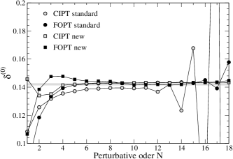
Figure 11: Values of $\delta^{(0)}$ for the model of Beneke and Jamin calculated with the CI and FO expansions, for $\alpha_{s}(m_{\tau}^{2})=0.26$.

7 Discussion

In this Section we make several more remarks on the expansions in powers of conformal mappings and their implications for the determination of $\alpha_{s}$. As discussed in Section 4, the definition of the optimal variable (13) requires only the knowledge of the location of the singularities of $B(u)$ in the Borel plane. The most general expansions based on the powers of the optimal variable are (16) and (27) for the CI and FO summations, respectively.

In the analysis presented in the previous Sections we used the modified expansions (20) and (30), generated by the Borel series (19) and (29) respectively, which explicitly include the nature of the lowest (leading) renormalon singularities in the Borel plane. It is of interest to consider also the general expansions (16) and (27), whose respective counterparts (15) and (26) do not manifestly display this singular behaviour. According to general arguments CiFi , we expect them to approach the true result, if the number of the perturbative terms is large enough. This is confirmed in Figs. 12 and 13, where we show the error of the determination of $\delta^{(0)}$ as a function of perturbative order $N$, for the standard CIPT and FOPT and the new expansions defined above.

For small $N$, the expansions (16) and (27) give results similar to the standard CI and FO expansions, while the expansions (20) and (30) approach much better the true result. This shows that at low $N$ the most important effect is the factorization of the singularities. However, for $N$ greater than 7 the effect of the conformal mapping becomes visible: as illustrated in Fig. 12, while the standard CI expansion starts to show large oscillations, the expansion (16) based on the conformal mapping of the complex Borel plane leads to only small oscillations around the true value. The improvement brought by the conformal mapping becomes visible rather slowly due to the strong leading IR singularity of the physical model considered in BeJa .

For the FO summation, the standard expansion starts to oscillate wildly for $N\geq 14$, while both modified expansions remain close to the true result. In this case, the approximation provided by the expansion (27), which does not include the nature of the singularities, turns out to be slightly better than the modified expansion (30). As discussed in Section 6, all the FO expansions provide a less satisfactory description of the Adler function near the timelike axis, but this region is suppressed in the integral (1).

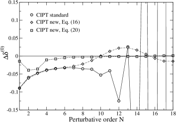
Figure 12: Error of the determination of $\delta^{(0)}$ as a function of perturbative order, for the standard and the new CI expansions.

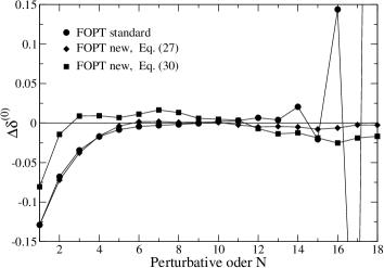
Figure 13: Error of the determination of $\delta^{(0)}$ as a function of perturbative order, for the standard and the new FO expansions.

The good approximations provided by the new CIPT (and, at points where the convergence of the series (6) is not poor, also by the new FOPT) can be explained qualitatively by a theorem proved in CiFi , which implies that the expansion (15) in powers of the variable $w$ has a better rate of convergence than the standard expansion (9) at points of the complex Borel plane where both converge. In particular, the convergence is better at points on the real positive axis below the first IR singularity, which gives the dominant contribution to the Laplace-Borel integral (8), due to the exponential factor that strongly suppresses the contribution of large $u$. Therefore, the improved expansion of $B(u)$ leads to a better approximation of the integral, at least for the perturbative orders investigated up to now. One might of course ask what happens if $N$ is further increased. It can be shown that going up to the 36th order the new CIPT continues to be stable, while the new FOPT somewhat deteriorates, and this is valid also for modified models, having, for instance, a smaller residue of the leading IR renormalon, compensated by an additional IR singularity that preserve the known low-order coefficients. However, a divergent behaviour at still higher orders is not excluded in principle, taking into account that the Laplace-Borel integral is performed along the cut, while the series (15) converges only at interior points. For a discussion of this problem and explicit criteria of convergence of the new expansion in the one-loop approximation of the coupling we refer to CaFi1 .

As mentioned in Section 4, the inclusion of the behaviour of $B(u)$ at the first branch points is not unique. Of course, for a large number of terms in the expansion the form of these factors is irrelevant, but at low orders one prescription may be better than the other. In (20) and (30), the dominant singular factors were expressed in the $w$ variable. Other possible expansions will be investigated elsewhere.

In order to test the choice made in this work, we use an idea applied in CaFi for illustrating the effect of conformal mappings on the convergence of power series. Consider the expansion (19) truncated after $N$ terms. The coefficients $c_{n}$, $n\leq N-1$, are calculated in a straightforward way from the first $N$ coefficients $K_{n}$, assumed to be known. When expanded as a Taylor series in the variable $u$, this expression reproduces the $N$ coefficients $K_{n}$ used as input, but contains also an infinity of higher order terms, in particular it predicts the next coefficient $K_{N+1}$. As an exercise, we used the expansion (19) with 4 terms, using as input the coefficients $K_{1}$ to $K_{4}$. The coefficients $c_{0}$ to $c_{3}$ are given in (37), the coefficients $c_{n}$ with $n\geq 4$ are set to zero. By reexpressing $B(u)$ from (19) as a series in powers of the $u$ variable, and using (9) and (10), we obtain $K_{5}=256$, which is quite close to the value $K_{5}=283$ adopted as a good estimate in BeJa . So, the expansion (19) is able to reproduce to a reasonable extent the higher order coefficients of the expanded function.

This nice feature is even more striking if we go one step further, using as input 5 coefficients $K_{n}$ from (3) and (4). Then we have 5 nonzero coefficients $c_{n}$, given in (37). By expanding $B(u)$ from (19) as a series in powers of $u$, we predict the higher coefficients $K_{6}=2929$, $K_{7}=1.73\cdot 10^{4}$, $K_{8}=3.14\cdot 10^{5}$, $K_{9}=9.23\cdot 10^{5}$, $K_{10}=6.34\cdot 10^{7}$, $K_{11}=-3.52\cdot 10^{8}$, $K_{12}=2.48\cdot 10^{10}$, which agree qualitatively with the values of the model of Beneke and Jamin BeJa , given in footnote 4. These apparently miraculous predictions are explained by the fact that the new expansion incorporates some features of the expanded function, which are known in advance. Then, with a smaller number of terms in the variable $w$, it reproduces well the higher order coefficients in the variable $u$.

Figure 14: Real part of $\hat{D}(s)$ for $s=m_{\tau}^{2}\rm{e}^{i\varphi}$ calculated with five perturbative terms in the new CIPT, Eq.(20), and new FOPT, Eq.(30).

Figure 15: Imaginary part of $\hat{D}(s)$ for $s=m_{\tau}^{2}\rm{e}^{i\varphi}$ calculated with five perturbative terms in the new CIPT, Eq.(20), and new FOPT, Eq.(30).

Finally, let us consider in more detail the predictions for $N=5$, which is the number of terms known in the physical case (recall that we adopted the value of $K_{5}$ used in BeJa ). As seen from Fig. 2, for $N=5$ the new CIPT and FOPT give results which approximate well the true value of $\delta^{(0)}$ from above and below, respectively. These results can be understood from the plots of the real and imaginary part of $\hat{D}(s)$ shown in Figs. 14-15. The new CIPT and FOPT approximate very well the true functions for large $\varphi$. For intermediate values of $\varphi$, CIPT and FOPT approach the true values comparatively well from opposite sides. For $\varphi$ close to 0, CIPT gives definitely a better approximation, but this region is suppressed in the integral (1). This explains why the resulting values of $\delta^{(0)}$ given by the new CIPT and FOPT are comparable.

8 Summary and conclusions

In this paper we applied a new perturbation series for QCD observables, proposed in CaFi , to the two renormalization group summations, CI and FO, used for the extraction of $\alpha_{s}$ from $\tau$ decays. The new expansion, which replaces the standard series in powers of the coupling, exploits in an optimal way the information about the high orders of perturbation theory. As discussed in detail in CaFi2 , the method separates the problem of convergence of the perturbation series from that of its ambiguity, solved by choosing a prescription, which is included in the definition the expansion functions (we adopt here the Principal Value).

In the present paper we worked out in detail the CI and FO versions of the new perturbation expansion for the Adler function in massless QCD. Also, a novelty is the incorporation of the singular behaviour of the Borel transform near the first branch points by factors in the new variable $w$, as shown in (19) and (29).

In Section 6 we illustrated the power of the new perturbation theory using as an example the model of Beneke and Jamin BeJa . As expected, the new CIPT proves to be superior, approaching the exact result to a very good accuracy when the perturbative order increases. The limitations of FOPT due to large imaginary logarithms along the integration contour in the complex plane are clearly illustrated.

From the predictions (38) and (40), adding an uncertainty of of 0.003 due to the power corrections BeJa , we obtain:

$$\alpha_{s}(m_{\tau}^{2})=0.3198\,^{+0.0113}_{-0.0094}\,,\quad{\rm new~{}CIPT},$$

$$\alpha_{s}(m_{\tau}^{2})=0.3113\,^{+0.0114}_{-0.0050}\,,\quad{\rm new~{}FOPT}.$$ (42)

As discussed in Section 5, the dominant contribution to the error is due to the uncertainty of the last perturbative term in the case of CIPT, and to the ambiguity of the renormalization scale in the case of FOPT.

It is remarkable that the difference between the central values in (8) is only $0.009$, while for the standard expansion the difference is $0.024$. The new expansions remove thus the most intriguing theoretical discrepancy in the determination of $\alpha_{s}$ from $\tau$ decays. We note that both values in (8) are closer to the standard FOPT than to the standard CIPT. So, our analysis indirectly confirms the criticism of the standard CIPT made in BeJa : although the renormalisation group summation is more accurate, the low order perturbative terms are not able to describe the high order features of the series. The new CIPT brings an improvement precisely at this point.

According to the last remark made in Section 7, for the model considered in BeJa the new CIPT and FOPT with $N=5$ terms give comparable predictions, which approximate the true result from opposite sides. If this model describes correctly the physical situation, then the true result is expected to be between the two predictions in (8). With this assumption, one may take the weighted average of these two values, which leads to

$$\alpha_{s}(m_{\tau}^{2})=0.315\,\,^{+0.008}_{-0.004}\,,\quad{\rm average}.$$ (43)

However, in order to avoid any bias related to a specific model, we take as best result the value given in (8) by the new CIPT:

$$\alpha_{s}(m_{\tau}^{2})=0.320\,^{+0.011}_{-0.009}\,.$$ (44)

We recall that this prediction is based on the new contour-improved expansion defined in Eq. (20). This expansion reproduces the known perturbative coefficients $K_{n}$ order by order, includes the information about the dominant singularities of the Adler function in the Borel plane, and is based on an optimal expansion of the Borel transform, which converges in the whole complex $u$-plane up to the cuts along the real axis.

The result (44) coincides practically with that obtained in BeJa using the standard FOPT. However, our prediction has a more solid theoretical basis, being free of fortuitous compensations of terms related to large imaginary logarithms, like in FOPT. Also, it is based on a systematic perturbation theory, and its uncertainty is related mainly to the error of the last perturbative term. So, the accuracy of the prediction is expected to increase when more perturbative terms for the Adler function in QCD will be available.

Acknowledgements: We are grateful to M. Jamin for providing us the RG-dependent coefficients of the expansion (6) and for very useful discussions. One of us (I.C.) thanks Prof. J. Chýla for hospitality at the Institute of Physics of the Czech Academy in Prague. This work was supported by the Romanian PN-II Programs Capacităţi of ANCS (Contract No. 15 EU/2009) and Idei of CNCSIS (Contract No. 464/2009), and by the Projects No. LA08015 of the Ministry of Education and AV0-Z10100502 of the Academy of Sciences of the Czech Republic.

References

- (1) C. Amsler et al., Phys. Lett. B667, 1 (2008).
- (2) E. Braaten, Phys. Rev. Lett. 60, 1606 (1988).
- (3) S. Narison, A. Pich, Phys. Lett. B211, 183 (1988).
- (4) A.A. Pivovarov, Z. Phys. C53, 461 (1992).
- (5) F. Le Diberder, A. Pich, Phys. Lett. B286, 147 (1992).
- (6) E. Braaten, S. Narison, A. Pich, Nucl. Phys. B373, 581 (1992).
- (7) P. Ball, M. Beneke, V.M. Braun, Nucl. Phys. B452, 563 (1995).
- (8) M. Neubert, Phys. Rev. D51, 5924 (1995).
- (9) B.V. Geshkenbein, B.L. Ioffe, K.N. Zyablyuk Phys.Rev. D64, 093009 (2001).
- (10) M. Jamin, JHEP 09, 058 (2005).
- (11) M. Davier, A. Höcker, Z. Zhang, Rev. Mod. Phys. 78, 1043 (2006).
- (12) K. Maltman, T. Yavin, Phys. Rev. D 78, 094020 (2008).
- (13) P.A. Baikov, K.G. Chetyrkin, J.H. Kühn, Phys. Rev. Lett. 101, 012002 (2008).
- (14) S.A. Larin, T. van Ritbergen and J.A.M. Vermaseren, Phys. Lett. B400, 379 (1997); Phys. Lett. B404, 153 (1997).
- (15) M. Czakon, Nucl. Phys. B 710, 485 (2005).
- (16) M. Davier, S. Descotes-Genon, Andreas Hocker, B. Malaescu, Z. Zhang, Eur.Phys.J.C56, 305 (2008).
- (17) M. Beneke, M. Jamin, JHEP 09, 044 (2008).
- (18) I. Caprini, J. Fischer, Phys. Rev. D60, 054014 (1999).
- (19) I. Caprini, J. Fischer, Phys. Rev. D62, 054007 (2000).
- (20) I. Caprini, J. Fischer, Eur.Phys.J.C 24, 127 (2002).
- (21) J. Fischer, J. Chýla, I. Caprini, Acta Phys. Slov. 52, 483 (2002).
- (22) A.L. Kataev and V.V. Starshenko, Mod. Phys. Lett. A10, 235 (1995).
- (23) P.A. Baikov, K.G. Chetyrkin, J.H. Kühn, Phys. Rev. D 67, 074026 (2003).
- (24) F.J. Dyson, Phys. Rev. 85, 631 (1952).
- (25) M. Beneke, Phys. Rep. 317, 1 (1999).
- (26) A. Mueller, Nucl.Phys. B250, 327 (1985).
- (27) M. Beneke, V.M. Braun, N. Kivel, Phys. Lett. B404, 315 (1997).
- (28) I. Caprini, M. Neubert, JHEP 03, 007 (1999).
- (29) I. Caprini and J. Fischer, Phys. Rev. D76, 018501 (2007).
- (30) S. Ciulli and J. Fischer, Nucl. Phys. 24, 465 (1961).
- (31) A.H. Mueller, in QCD - Twenty Years Later, Aachen 1992, edited by P. Zerwas and H. A. Kastrup (World Scientific, Singapore, 1992).
- (32) G. Altarelli, P. Nason, G. Ridolfi, Z. Phys. C68, 257 (1995).
- (33) U.D. Jentschura, E. J. Weniger, G. Soff, J. Phys. G26, 1545 (2000).
- (34) G. Cvetič, T. Lee, Phys. Rev D54, 014030 (2001).
- (35) D.E. Soper, L.R. Surguladze, Phys. Rev. D54, 4566 (1996).