High Dimensional Nonlinear Learning using Local Coordinate Coding

Abstract

This paper introduces a new method for semi-supervised learning on high dimensional nonlinear manifolds, which includes a phase of unsupervised basis learning and a phase of supervised function learning. The learned bases provide a set of anchor points to form a local coordinate system, such that each data point $x$ on the manifold can be locally approximated by a linear combination of its nearby anchor points, with the linear weights offering a local-coordinate coding of $x$. We show that a high dimensional nonlinear function can be approximated by a global linear function with respect to this coding scheme, and the approximation quality is ensured by the locality of such coding. The method turns a difficult nonlinear learning problem into a simple global linear learning problem, which overcomes some drawbacks of traditional local learning methods. The work also gives a theoretical justification to the empirical success of some biologically-inspired models using sparse coding of sensory data, since a local coding scheme must be sufficiently sparse. However, sparsity does not always satisfy locality conditions, and can thus possibly lead to suboptimal results. The properties and performances of the method are empirically verified on synthetic data, handwritten digit classification, and object recognition tasks.

1 Introduction

Consider the problem of learning a nonlinear function $f(x)$ in high dimension: $x\in{\mathbb{R}}^{d}$ with large $d$. We are given a set of labeled data $(x_{1},y_{1}),\ldots,(x_{n},y_{n})$ drawn from an unknown underlying distribution. Moreover, assume that we observe a set of unlabeled data $x\in{\mathbb{R}}^{d}$ from the same distribution. If the dimensionality $d$ is large compared to $n$, then the traditional statistical theory predicts over-fitting due to the so called “curse of dimensionality”. One intuitive argument for this effect is that when the dimensionality becomes larger, pairwise distances between two similar data points become larger as well. Therefore one needs more data points to adequately fill in the empty space. However, for many real problems with high dimensional data, we do not observe this so-called curse of dimensionality. This is because although data are physically represented in a high-dimensional space, they often (approximately) lie on a manifold which has a much smaller intrinsic dimensionality.

This paper proposes a new method that can take advantage of the manifold geometric structure to learn a nonlinear function in high dimension. The main idea is to locally embed points on the manifold into a lower dimensional space, expressed as coordinates with respect to a set of anchor points. Our main observation is simple but very important: we show that a nonlinear function on the manifold can be effectively approximated by a linear function with such a coding under appropriate localization conditions. Therefore by using Local Coordinate Coding, we turn a very difficult high dimensional nonlinear learning problem into a much simpler linear learning problem, which has been extensively studied in the literature. This idea may also be considered as a high dimensional generalization of low dimensional local smoothing methods in the traditional statistical literature.

2 Local Coordinate Coding

We are interested in learning a smooth function $f(x)$ defined on a high dimensional space ${\mathbb{R}}^{d}$. Let $\|\cdot\|$ be a norm on ${\mathbb{R}}^{d}$. Although we do not restrict to any specific norm, in practice, one often employs the Euclidean norm (2-norm): $\|x\|=\|x\|_{2}=\sqrt{x_{1}^{2}+\cdots+x_{d}^{2}}$.

Definition 2.1 (Lipschitz Smoothness)

A function $f(x)$ on ${\mathbb{R}}^{d}$ is $(\alpha,\beta,p)$-Lipschitz smooth with respect to a norm $\|\cdot\|$ if

$$|f(x^{\prime})-f(x)|\leq\alpha\|x-x^{\prime}\|,$$

and

$$|f(x^{\prime})-f(x)-\nabla f(x)^{\top}(x^{\prime}-x)|\leq\beta\|x-x^{\prime}\|^{1+p},$$

where we assume $\alpha,\beta>0$ and $p\in(0,1]$.

Note that if the Hessian of $f(x)$ exists, then we may take $p=1$. Learning an arbitrary Lipschitz smooth function on ${\mathbb{R}}^{d}$ can be difficult due to the curse of dimensionality. That is, the number of samples required to characterize such a function $f(x)$ can be exponential in $d$. However, in many practical applications, one often observes that the data we are interested in lie approximately on a manifold ${\cal M}$ which is embedded into ${\mathbb{R}}^{d}$. Although $d$ is large, the intrinsic dimensionality of ${\cal M}$ can be much smaller. Therefore if we are only interested in learning $f(x)$ on ${\cal M}$, then the complexity should depend on the intrinsic dimensionality of ${\cal M}$ instead of $d$.

In this paper, we approach this problem by introducing the idea of localized coordinate coding. The formal definition of (non-localized) coordinate coding is given below, where we represent a point in ${\mathbb{R}}^{d}$ by a linear combination of a set of “anchor points”. Later we show it is sufficient to choose a set of “anchor points” with cardinality depending on the intrinsic dimensionality of the manifold rather than $d$.

Definition 2.2 (Coordinate Coding)

A coordinate coding is a pair $(\gamma,C)$, where $C\subset{\mathbb{R}}^{d}$ is a set of anchor points, and $\gamma$ is a map of $x\in{\mathbb{R}}^{d}$ to $[\gamma_{v}(x)]_{v\in C}\in R^{|C|}$ such that $\sum_{v}\gamma_{v}(x)=1$. It induces the following physical approximation of $x$ in ${\mathbb{R}}^{d}$:

$$\gamma(x)=\sum_{v\in C}\gamma_{v}(x)v.$$

Moreover, for all $x\in{\mathbb{R}}^{d}$, we define the coding norm as

$$\|x\|_{\gamma}=\left(\sum_{v\in C}\gamma_{v}(x)^{2}\right)^{1/2}.$$

The quantity $\|x\|_{\gamma}$ will become useful in our learning theory analysis. The condition $\sum_{v}\gamma_{v}(x)=1$ follows from the shift-invariance requirement, which means that the coding should remain the same if we use a different origin of the ${\mathbb{R}}^{d}$ coordinate system for representing data points. However, if in practice we can find a good origin for the global coordinate system in ${\mathbb{R}}^{d}$, and if all points on ${\cal M}$ are close to it, then the shift-invariance requirement may become less important.

Proposition 2.1

The map $x\to\sum_{v\in C}\gamma_{v}(x)v$ is invariant under any shift of the origin for representing data points in ${\mathbb{R}}^{d}$ if and only if $\sum_{v}\gamma_{v}(x)=1$.

The importance of the coordinate coding concept is that if a coordinate coding is sufficiently localized, then a nonlinear function can be approximate by a linear function with respect to the coding. This critical observation, illustrate in the following linearization lemma, is the foundation of our approach.

Lemma 2.1 (Linearization)

Let $(\gamma,C)$ be an arbitrary coordinate coding on ${\mathbb{R}}^{d}$. Let $f$ be an $(\alpha,\beta,p)$-Lipschitz smooth function. We have for all $x\in{\mathbb{R}}^{d}$:

$$\left|f(x)-\sum_{v\in C}\gamma_{v}(x)f(v)\right|\leq\alpha\left\|x-\gamma(x)\right\|+\beta\sum_{v\in C}|\gamma_{v}(x)|\left\|v-\gamma(x)\right\|^{1+p}.$$

To understand this result, we note that on the left hand side, a nonlinear function $f(x)$ in $R^{d}$ is approximated by a linear function $\sum_{v\in C}\gamma_{v}(x)f(v)$ with respect to the coding $\gamma(x)$, where $[f(v)]_{v\in C}$ is the set of coefficients to be estimated from data. The quality of this approximation is bounded by the right hand side, which has two terms: the first term $\|x-\gamma(x)\|$ means $x$ should be close to its physical approximation $\gamma(x)$, and the second term means that the coding should be localized. The quality of a coding $\gamma$ with respect to $C$ can be measured by the right hand side. For convenience, we introduce the following definition, which measures the locality of a coding.

Definition 2.3 (Localization Measure)

Given $\alpha,\beta,p$, and coding $(\gamma,C)$, we define

$$Q_{\alpha,\beta,p}(\gamma,C)={\mathbb{E}}_{x}\left[\alpha\|x-\gamma(x)\|+\beta\sum_{v\in C}|\gamma_{v}(x)|\left\|v-\gamma(x)\right\|^{1+p}\right].$$

Observe that in $Q_{\alpha,\beta,p}$, $\alpha,\beta,p$ may be regarded as tuning parameters; we may also simply pick $\alpha=\beta=p=1$. Since the quality function $Q_{\alpha,\beta,p}(\gamma,C)$ only depends on unlabeled data, in principle, we can find $[\gamma,C]$ by optimizing this quality using unlabeled data. Later, we will consider simplifications of this objective function that are easier to compute.

Next we show that if the data lie on a manifold, then the complexity of local coordinate coding depends on the intrinsic manifold dimensionality instead of $d$. We first define manifold and its intrinsic dimensionality.

Definition 2.4 (Manifold)

A subset ${\cal M}\subset{\mathbb{R}}^{d}$ is called a $p$-smooth ($p>0$) manifold with intrinsic dimensionality $m=m({\cal M})$ if there exists a constant $c_{p}({\cal M})$ such that given any $x\in{\cal M}$, there exists $m$ vectors $v_{1}(x),\ldots,v_{m}(x)\in{\mathbb{R}}^{d}$ so that $\forall x^{\prime}\in{\cal M}$:

$$\inf_{\gamma\in{\mathbb{R}}^{m}}\left\|x^{\prime}-x-\sum_{j=1}^{m}\gamma_{j}v_{j}(x)\right\|\leq c_{p}({\cal M})\|x^{\prime}-x\|^{1+p}.$$

This definition is quite intuitive. The smooth manifold structure implies that one can approximate a point in ${\cal M}$ effectively using local coordinate coding. Note that for a typical manifold with well-defined curvature, we can take $p=1$.

Definition 2.5 (Covering Number)

Given any subset ${\cal M}\subset{\mathbb{R}}^{d}$, and $\epsilon>0$. The covering number, denoted as ${\cal N}(\epsilon,{\cal M})$, is the smallest cardinality of an $\epsilon$-cover $C\subset{\cal M}$. That is,

$$\sup_{x\in{\cal M}}\inf_{v\in C}\|x-v\|\leq\epsilon.$$

For a compact manifold with intrinsic dimensionality $m$, there exists a constant $c({\cal M})$ such that its covering number is bounded by

$${\cal N}(\epsilon,{\cal M})\leq c({\cal M})\epsilon^{-m}.$$

The usual statistical definition of dimensionality only involves the covering number $|C|$. However, the manifold intrinsic dimensionality is also important by itself in our analysis.

The following result shows that there exists a local coordinate coding to a set of anchor points $C$ of cardinality $O(m({\cal M}){\cal N}(\epsilon,{\cal M}))$ such that any $(\alpha,\beta,p)$-Lipschitz smooth function can be linearly approximated using local coordinate coding up to the accuracy $O(\sqrt{m({\cal M})}\epsilon^{1+p})$.

Theorem 2.1 (Manifold Coding)

If the data points $x$ lie on a compact $p$-smooth manifold ${\cal M}$, and the norm is defined as $\|x\|=(x^{\top}Ax)^{1/2}$ for some positive definite matrix $A$. Then given any $\epsilon>0$, there exist anchor points $C\subset{\cal M}$ and coding $\gamma$ such that

$$|C|\leq(1+m){\cal N}(\epsilon,{\cal M}),$$

$$Q_{\alpha,\beta,p}(\gamma,C)\leq[\alpha c_{p}({\cal M})+(1+\sqrt{m}+2^{1+p}\sqrt{m})\beta]\,\epsilon^{1+p},$$

where $m=m({\cal M})$. Moreover, for all $x\in{\cal M}$, we have $\|x\|_{\gamma}^{2}\leq 1+(1+\sqrt{m})^{2}$.

The approximation result in Theorem 2.1 means that the complexity of linearization in Lemma 2.1 depends only on the intrinsic dimension $m({\cal M})$ of ${\cal M}$ instead of $d$. Although this result is proved for manifolds, it is important to observe that the coordinate coding method proposed in this paper does not require the data to lie precisely on a manifold, and it does not require knowing $m({\cal M})$. In fact, similar results hold even when the data only approximately lie on a manifold.

In the next section, we characterize the learning complexity of the local coordinate coding method. It implies that linear prediction methods can be used to effectively learn nonlinear functions on a manifold. The nonlinearity is fully captured by the coordinate coding map $\gamma$ (which can be a nonlinear function). This approach has some great advantages because the problem of learning local-coordinate coding is much simpler than direct nonlinear learning:

• Learning $(\gamma,C)$ only requires unlabeled data, and the number of unlabeled data can be significantly more than the number of labeled data. This also prevents overfitting with respect to labeled data.

• In practice, we do not have to find the optimal coding because the coordinates are merely features for linear supervised learning. This significantly simplifies the optimization problem. Consequently, it is more robust than standard approaches to nonlinear learning that direct optimize nonlinear functions on labeled data (e.g., neural networks).

3 Learning Theory

In machine learning, we minimize the expected loss $\phi(f(x),y)$ with respect to the underlying distribution

$${\mathbb{E}}_{x,y}\phi(f(x),y)$$

within a function class $f(x)\in{\cal F}$. In this paper, we are interested in the function class

$${\cal F}_{\alpha,\beta,p}=\{f(x):(\alpha,\beta,p)-\text{Lipschitz smooth function in }{\mathbb{R}}^{d}\}.$$

The local coordinate coding method considers a linear approximation of functions in ${\cal F}_{\alpha,\beta,p}$ on the data manifold. Given a local-coordinate coding scheme $(\gamma,C)$, we approximate each $f(x)\in{\cal F}_{\alpha,\beta,p}^{a}$ by

$$f(x)\approx f_{\gamma,C}(\hat{w},x)=\sum_{v\in C}\hat{w}_{v}\gamma_{v}(x),$$

where we estimate the coefficients using ridge regression as:

$$[\hat{w}_{v}]=\arg\min_{[w_{v}]}\left[\sum_{i=1}^{n}\phi\left(f_{\gamma,C}(w,x_{i}),y_{i}\right)+\lambda\sum_{v\in C}w_{v}^{2}\right].$$ (1)

Given a loss function $\phi(p,y)$, let $\phi_{1}^{\prime}(p,y)=\partial\phi(p,y)/\partial p$. For simplicity, in this paper we only consider convex Lipschitz loss function, where $|\phi_{1}^{\prime}(p,y)|\leq B$. This includes the standard classification loss functions such as logistic regression and SVM (hinge loss), both with $B=1$.

Theorem 3.1 (Generalization Bound)

Suppose $\phi(p,y)$ is Lipschitz: $|\phi_{1}^{\prime}(p,y)|\leq B$. Consider coordinate coding $(\gamma,C)$, and the estimation method (1) with random training examples $S_{n}=\{(x_{1},y_{1}),\ldots,(x_{n},y_{n})\}$. Then the expected generalization error satisfies the inequality:

$${\mathbb{E}}_{S_{n}}\;{\mathbb{E}}_{x,y}\phi(f_{\gamma,C}(\hat{w},x),y)$$

$$\leq \inf_{f\in{\cal F}_{\alpha,\beta,p}}\left[{\mathbb{E}}_{x,y}\phi\left(f(x),y\right)+\lambda\sum_{v\in C}f(v)^{2}\right]+\frac{B^{2}}{2\lambda n}{\mathbb{E}}_{x}\|x\|_{\gamma}^{2}+BQ_{\alpha,\beta,p}(\gamma,C).$$

If we choose the regularization parameter $\lambda$ that optimizes the bound, then the right hand side becomes

$$\inf_{f\in{\cal F}_{\alpha,\beta,p}}\left[{\mathbb{E}}_{x,y}\phi\left(f(x),y\right)+B\sqrt{\frac{2}{n}\sum_{v\in C}f(v)^{2}\;{\mathbb{E}}_{x}\|x\|_{\gamma}^{2}}\right]+BQ_{\alpha,\beta,p}(\gamma,C).$$ (2)

In particular, if we find $(\gamma,C)$ at some $\epsilon>0$, then Theorem 2.1 implies the following simplification for any $f\in{\cal F}_{\alpha,\beta,p}$ such that $|f(x)|\leq A$ for a fixed constant $A$, then the bound on the generalization error becomes:

$${\mathbb{E}}_{x,y}\phi\left(f(x),y\right)+O\left[\sqrt{\epsilon^{-m({\cal M})}/n}+\epsilon^{1+p}\right].$$

By optimizing over $\epsilon$, we obtain a bound: ${\mathbb{E}}_{x,y}\phi\left(f(x),y\right)+O(n^{-(1+p)/(2+2p+m({\cal M}))})$.

By combining Theorem 2.1 and Theorem 3.1, we can immediately obtain the following simple consistency result. It shows that the algorithm can learn an arbitrary nonlinear function on manifold when $n\to\infty$. Note that Theorem 2.1 implies that the convergence only depends on the intrinsic dimensionality of the manifold ${\cal M}$, not $d$.

Theorem 3.2 (Consistency)

Suppose the data lie on a compact manifold ${\cal M}\subset{\mathbb{R}}^{d}$, and the norm $\|\cdot\|$ is the Euclidean norm in ${\mathbb{R}}^{d}$. If loss function $\phi(p,y)$ is Lipschitz. As $n\to\infty$, we choose $\alpha,\beta\to\infty$, $\alpha/n,\beta/n\to 0$ ($\alpha,\beta$ depends on $n$), and $p=0$. Then it is possible to find coding $(\gamma,C)$ using unlabeled data such that $|C|/n\to 0$ and $Q_{\alpha,\beta,p}(\gamma,C)\to 0$. If we pick $\lambda n\to\infty$, and $\lambda|C|\to 0$. Then the local coordinate coding method (1) is consistent as $n\to\infty$:

$$\lim_{n\to\infty}{\mathbb{E}}_{S_{n}}\;{\mathbb{E}}_{x,y}\phi(f(\hat{w},x),y)=\inf_{f:{\cal M}\to{\mathbb{R}}}{\mathbb{E}}_{x,y}\phi\left(f(x),y\right).$$

4 Practical Learning of Coding

Given a coordinate coding $(\gamma,C)$, we can use (1) to learn a nonlinear function in ${\mathbb{R}}^{d}$. We showed that $(\gamma,C)$ can be obtained by optimizing $Q_{\alpha,\beta,p}(\gamma,C)$. In practice, we may also consider the following simplifications of the localization term:

$$\sum_{v\in C}|\gamma_{v}(x)|\left\|v-\gamma(x)\right\|^{1+p}\approx\sum_{v\in C}|\gamma_{v}(x)|\left\|v-x\right\|^{1+p}.$$

Note that we may simply chose $p=0$ or $p=1$. The formulation is related to sparse coding [4] which has no locality constraints with $p=-1$. In this representation, we may either enforce the constraint $\sum_{v}\gamma_{v}(x)=1$ or remove it for simplicity (in such case, we assume that the coordinate origin is appropriately chosen so that the shift-invariance requirement is not important). Putting the above together, we try to optimize the following objective function in practice:

$$Q(\gamma,C)={\mathbb{E}}_{x}\inf_{[\gamma_{v}]}\left[\left\|x-\sum_{v\in C}\gamma_{v}v\right\|^{2}+\mu\sum_{v\in C}|\gamma_{v}|\|v-x\|^{2}\right].$$

5 Relationship to Other Methods

Our work is related to several existing approaches in the literature of machine learning and statistics. The first class of them is nonlinear manifold learning, such as LLE [5], Isomap [6], and Laplacian Eigenmaps [1]. These methods find global coordinates of data manifold based on a pre-computed affinity graph of data points. The use of affinity graphs requires expensive computation and lacks a coherent way of generalization to new data. Our method learns a compact set of bases to form local coordinates, which has a linear complexity with respect to data size and can naturally handle unseen data. More importantly, local coordinate coding has a direct connection to function approximation on manifold, and thus provides a sound unsupervised pre-training method to facilitate further supervised learning tasks.

Another set of related models are local models in statistics, such as local kernel smoothing and local regression, both traditionally using fixed-bandwidth kernels. Local kernel smoothing can be regarded as a zero-order method; while local regression is higher-order, including local linear regression as the 1st-order case. Traditional local methods are not widely used in machine learning practice, because data with non-uniform distribution on the manifold require to use adaptive-bandwidth kernels. The problem can be somehow alleviated by using $K$-nearest neighbors. However, adaptive kernel smoothing still suffers from the high-dimensionality and noise of data. On the other hand, higher-order methods are computationally expensive and prone to overfitting, because they are highly flexible in locally fitting many segments of data in high-dimensional spaces. Our method can be seen as a generalized 1st-order local method with basis learning and adaptive locality. Compared to local linear regression, the learning is achieved by fitting a single globally linear function with respect to a set of learned local coordinates, which is much less prone to overfitting and computationally much cheaper. This means that our method achieves better balance between local and global aspects of learning. The importance of such balance has been recently discussed in [7].

Finally, local-coordinate coding draws connections to vector quantization (VQ) coding and sparse coding, which have been widely applied in processing of sensory data, such as acoustic and image signals. Learning linear functions of VQ codes can be regarded as a generalized zero-order local method with adaptive basis learning. Our method has an intimate relationship with sparse coding. In fact, we can regard local coordinate coding as locally constrained sparse coding. Inspired by biological visual systems, people has been arguing sparse features of signals are useful for learning [4]. However, to the best of our knowledge, there is no analysis in the literature that directly answers the question why sparse codes can help learning nonlinear functions in high dimensional spaces. Our work reveals an important finding — a good first-order approximation to nonlinear function requires the codes to be local, which consequently requires the codes to be sparse. However, sparsity does not always guarantee locality conditions. Our experiments demonstrate that sparse coding is helpful for learning only when the codes are local. Therefore locality is more essential for coding, and sparsity is a consequence of such a condition.

Properties of related methods discussed in this section are compared in Table 1.

method	dimension	basis learning	approximation power
kernel smoothing	low	no	0th order
local linear regression	low	no	1st order
$K$-nearest neighbor	high	no	0th order
Vector Quantization (VQ)	high	yes	0th order
Local Coordinate Coding (LCC)	high	yes	1st order

Table 1: Comparison of Related Methods

6 Experiments

We use three experiments to demonstrate various points of the theoretical claims. In particular, the importance of coding locality and the robustness of various methods to high data dimensionality.

6.1 Synthetic Data

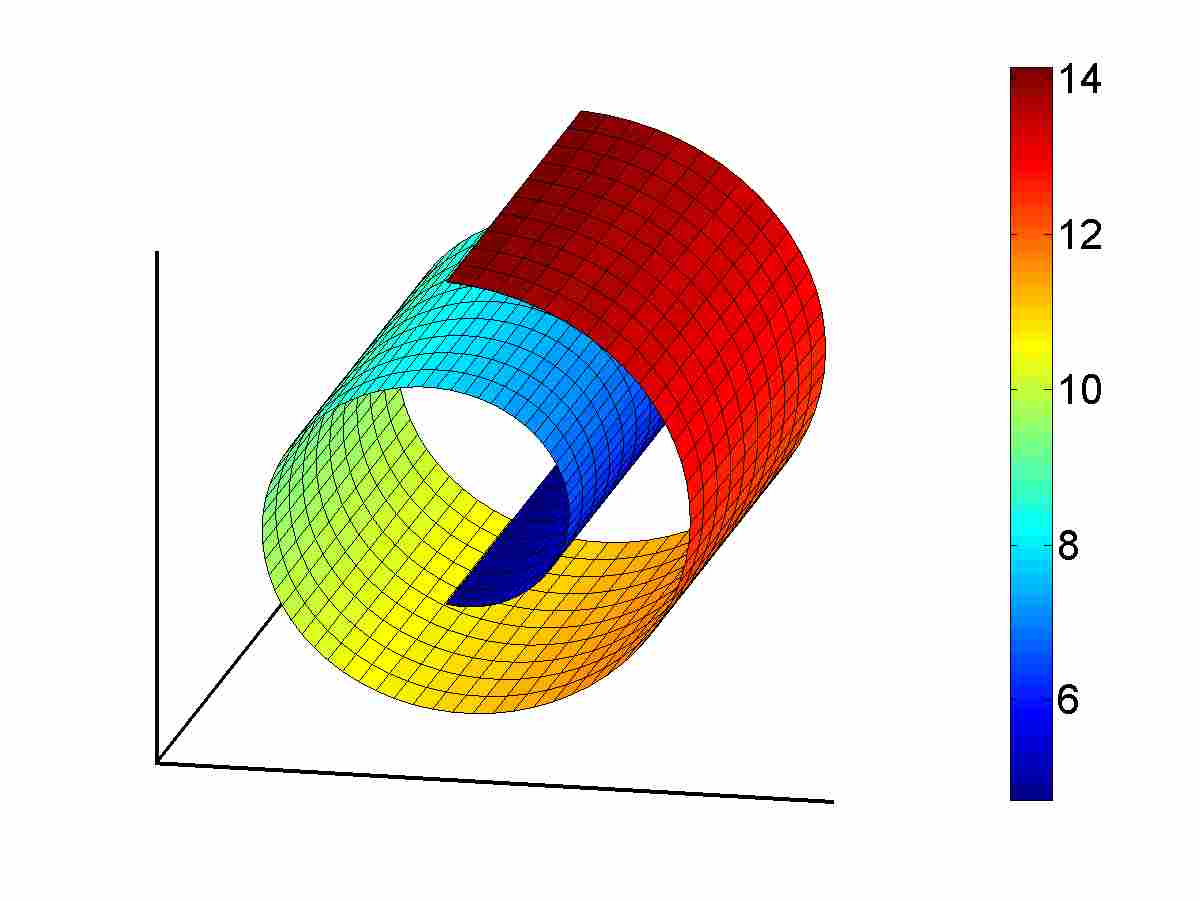
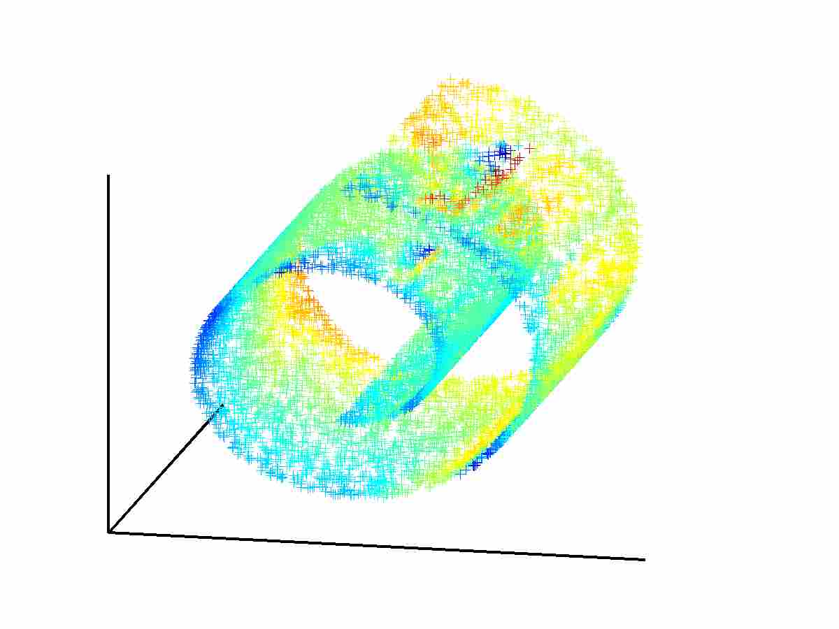
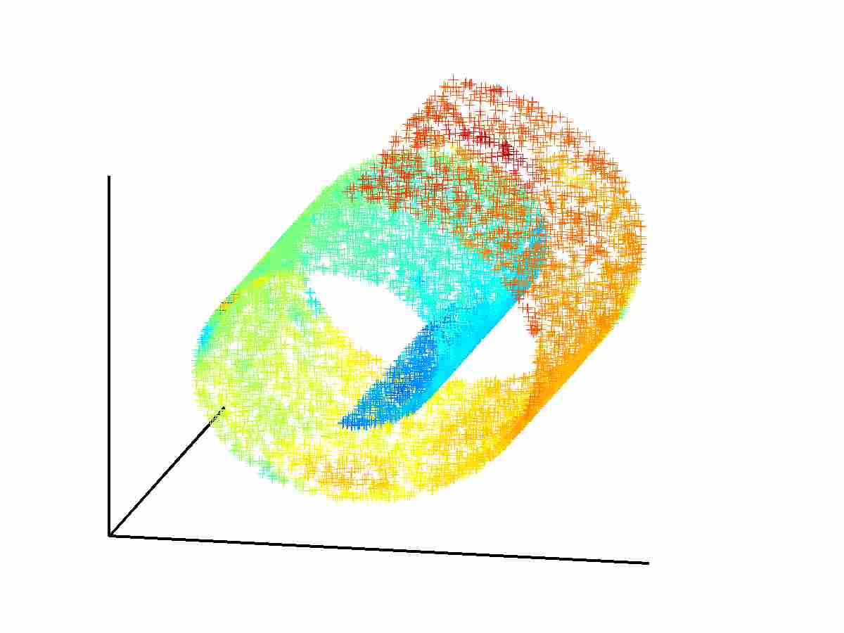
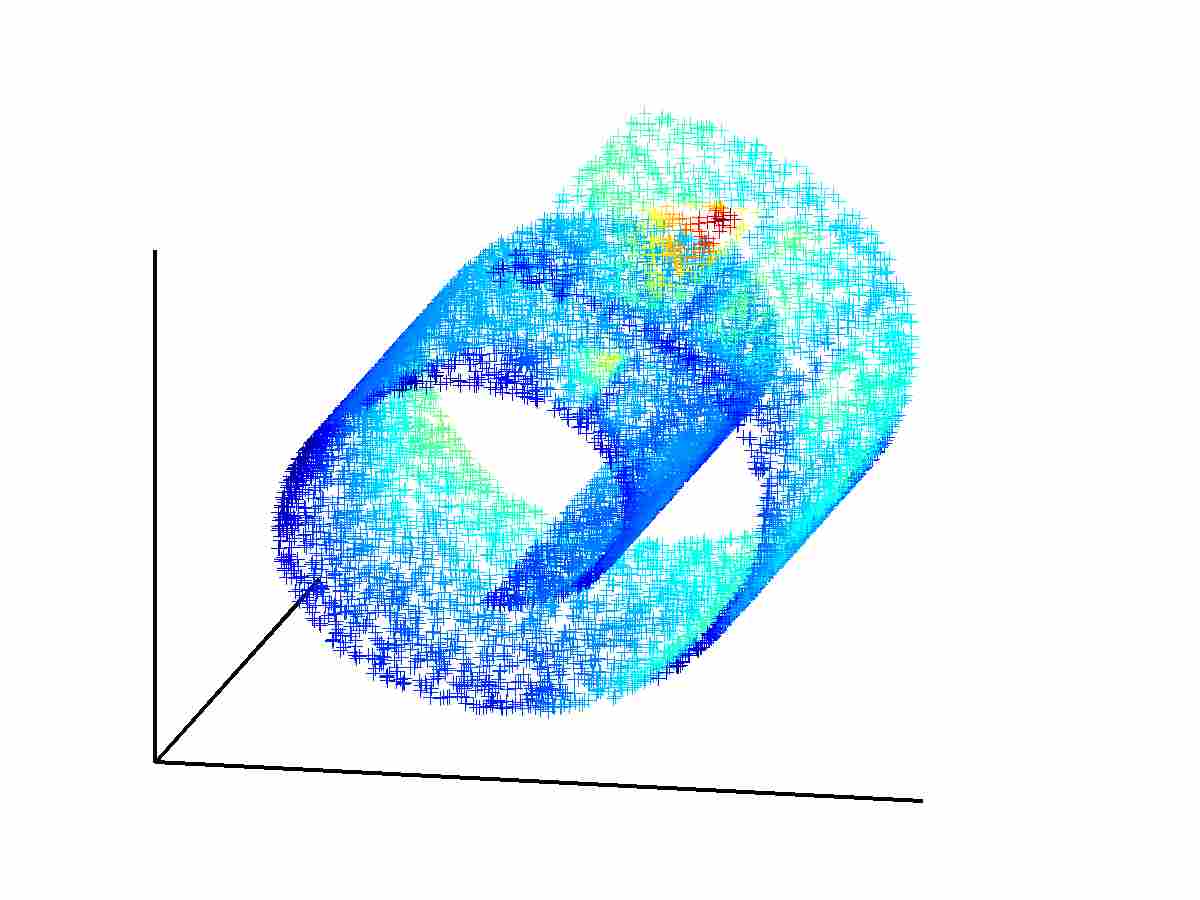
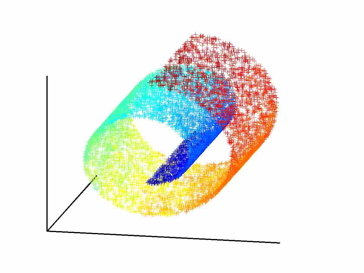
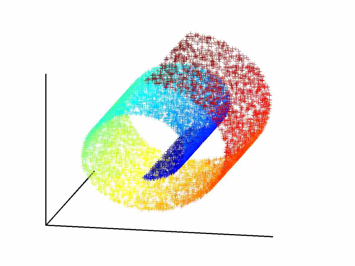
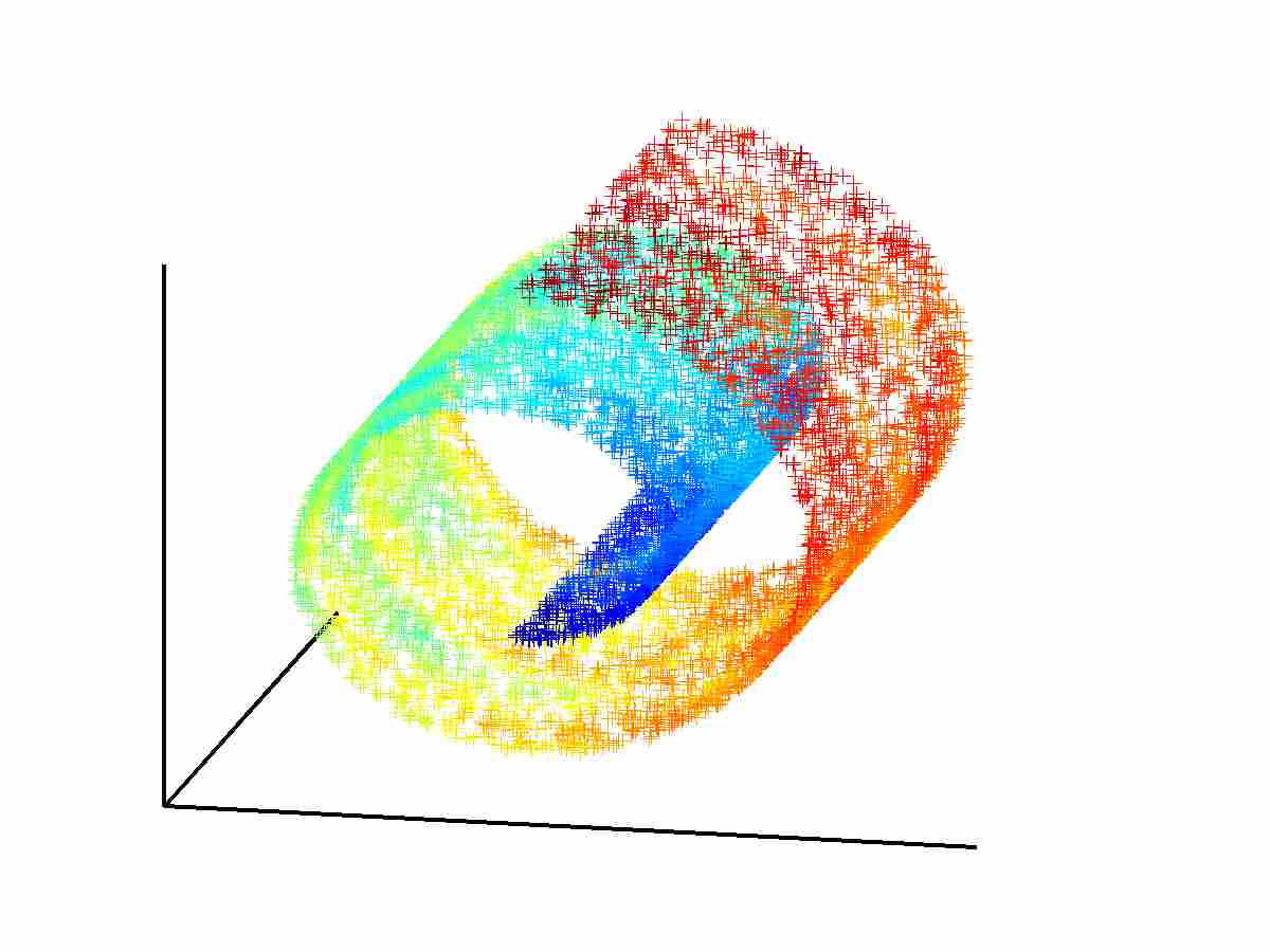
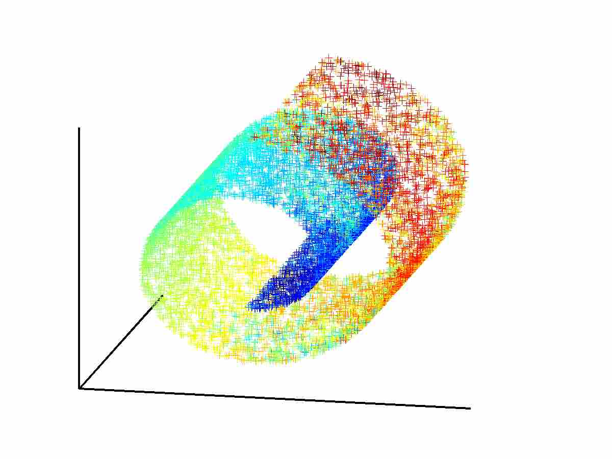
Our first experiment is based on a synthetic data set, where a nonlinear function is defined on a Swiss-roll manifold, as shown in Figure 1-(1). The primary goal is to demonstrate the performance of nonlinear function learning using simple linear ridge regression based on representations obtained from traditional sparse coding and the newly suggested local coordinate coding, which are, respectively, formulated as the following,

$$\min_{\gamma,C}~{}\sum_{x}\frac{1}{2}\left\|x-\gamma(x)\right\|^{2}+\beta\sum_{v\in C}|\gamma_{v}(x)|+\lambda\sum_{v\in C}\|v\|^{2}$$ (3)

$$\min_{\gamma,C}~{}\sum_{x}\frac{1}{2}\left\|x-\gamma(x)\right\|^{2}+\beta\sum_{v\in C}|\gamma_{v}(x)|\|v-x\|^{2}+\lambda\sum_{v\in C}\|v\|^{2}$$ (4)

where $\gamma(x)=\sum_{v\in C}\gamma_{v}(x)v$. We note that (4) is an approximation to the original formulation, mainly for the simplicity of computation.

We randomly sample $50,000$ data points on the manifold for unsupervised basis learning, and $500$ labeled points for supervised regression. The number of bases is fixed to be 128. The learned nonlinear functions are tested on another set of $10,000$ data points, with their performances evaluated by root mean square error (RMSE).

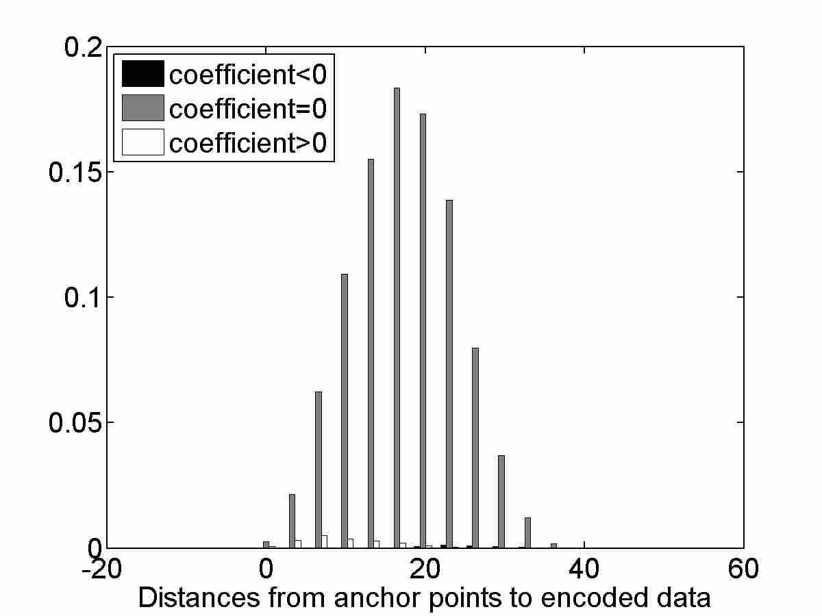
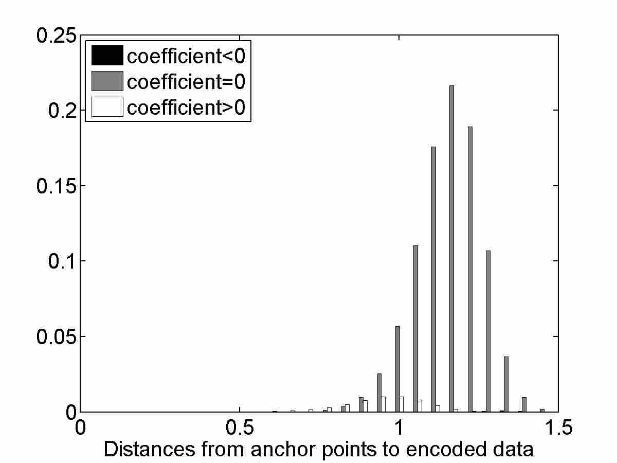
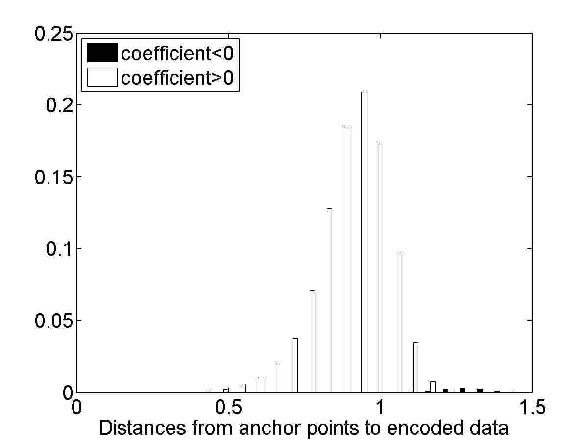
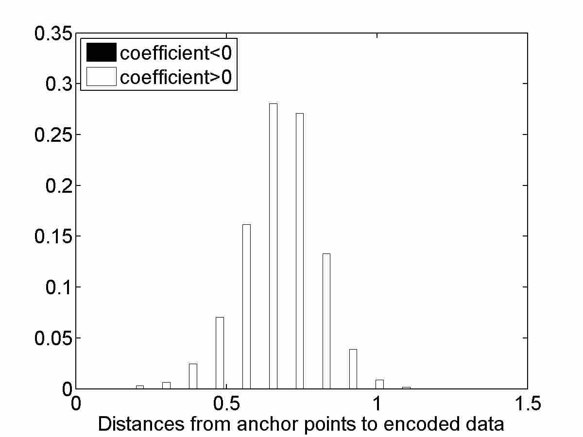
In the first setting, we let both coding methods use the same set of fixed bases, which are 128 points randomly sampled from the manifold. The regression results are shown in Figure 1-(2) and (3), respectively. Sparse coding based approach fails to capture the nonlinear function, while local coordinate coding behaves much better. We take a closer look at the data representations obtained from the two different encoding methods, by visualizing the distributions of distances from encoded data to bases that have positive, negative, or zero coefficients in Figure 2. It shows that sparse coding lets bases faraway from the encoded data have nonzero coefficients, while local coordinate coding allows only nearby bases to get nonzero coefficients. In other words, sparse coding on this data does not ensure a good locality and thus fails to facilitate the nonlinear function learning. As another interesting phenomenon, local coordinate coding seems to encourage coefficients to be nonnegative, which is intuitively understandable — if we use several bases close to a data point to linearly approximate the point, each basis should have a positive contribution. However, whether there is any merit by explicitly enforcing non-negativity will remain an interesting future work.

In the next, given the random bases as a common initialization, we let the two algorithms learn bases from the $50,000$ unlabeled data points. The regression results based on the learned bases are depicted in Figure 1-(4) and (5), which indicate that regression error is further reduced for local coordinate coding, but remains to be high for sparse coding. We also make a comparison with local kernel smoothing, which takes a weighted average of function values of $K$-nearest training points to make prediction. As shown in Figure 1-(6), the method works very well on this simple low-dimensional data, even outperforming the local coordinate coding approach. However, if we increase the data dimensionality to be $256$ by adding $253$-dimensional independent Gaussian noises with zero mean and unitary variance, local coordinate coding becomes superior to local kernel smoothing, as shown in Figure 1-(7) and (8). This is consistent with our theory, which suggests that local coordinate coding can work well in high dimension; on the other hand, local kernel smoothing is known to suffer from high dimensionality and noise.

(1) A nonlinear function	(2) RMSE=$4.394$	(3) RMSE=$0.499$	(4)RMSE=$4.661$
(5) RMSE=$0.201$	(6) RMSE=$0.109$	(7) RMSE=$0.669$	(8) RMSE=$1.170$

Figure 1: Experiments of nonlinear regression on the Swiss-roll data: (1) a nonlinear function on the Swiss-roll manifold, where the color indicates function values; (2) result of sparse coding with fixed random anchor points; (3) result of local coordinate coding with fixed random anchor points; 4) result of sparse coding; (5) result of local coordinate coding; (6) result of local kernel smoothing; (7) result of local coordinate coding on noisy data; (8) result of local kernel smoothing on noisy data.

(a-1)	(a-2)
(b-1)	(b-2)

Figure 2: Coding locality on Swiss roll: (a) sparse coding vs. (b) local coordinate coding.

6.2 Handwritten Digit Recognition

Our second experiment is based on the MNIST handwritten digit recognition benchmark, where each data point is a $28\times 28$ gray image, and pre-normalized into a unitary $784$-dimensional vector. In our setting, the set $C$ of anchor points is obtained from sparse coding, whose formulation follows (3), with the regularization on $v$ replaced by inequality constraints $\|v\|\leq 1$. Our focus here is not on anchor point learning, but rather on checking whether a good nonlinear classifier can be obtained if we enforce sparsity and locality in data representation, and then apply simple one-against-call linear SVMs.

Figure 3: The anchor points of MNIST digits ($|C|=512$).

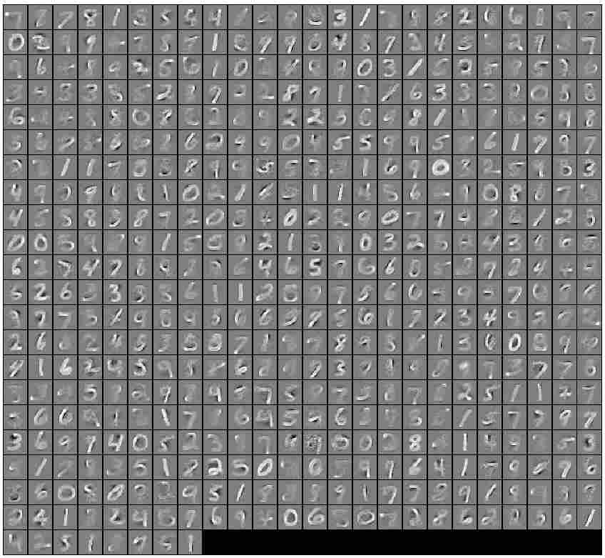
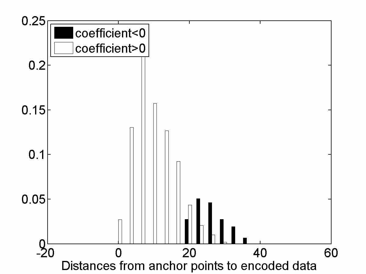
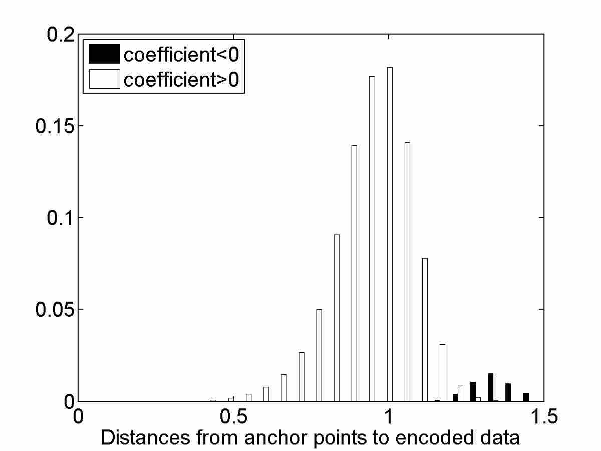
Since the optimization cost of sparse coding is invariant under flipping the sign of $v$, we take a post-processing step to change the sign of $v$ if we find the corresponding $\gamma_{v}(x)$ for most of $x$ is negative. This rectification will ensure the anchor points to be on the data manifold. One example of $C$ is visualized in Figure 3, where the number of anchor points is $|C|=512$. With the obtained $C$, for each data point $x$ we solve the local coordinate coding problem (4), by optimizing $\gamma$ only, to obtain the representation $[\gamma_{v}(x)]_{v\in C}$. In the experiments we try different sizes of bases. The classification error rates are provided in Table 2. In addition we also compare with linear classifier on raw images, local kernel smoothing based on $K$-nearest neighbors, and linear classifiers using representations obtained from various unsupervised learning methods, including auto-encoder based on deep belief networks, Laplacian eigenmaps [1], and VQ coding based on $K$-means. We note that, like most of other manifold learning approaches, Laplacian eigenmaps is a transductive method which has to incorporate both training and testing data in training. The comparison results are summarized in Table 3. Both sparse coding and local coordinate coding perform quite good for this nonlinear classification task, significantly outperforming linear classifiers on raw images. In addition, local coordinate coding is consistently better than sparse coding across various basis sizes. We further check the locality of both representations by plotting Figure-4, where the basis number is $512$, and find that sparse coding on this data set happens to be quite local — unlike the case of Swiss-roll data — here only a small portion of nonzero coefficients (again mostly negative) are assigned onto the bases whose distances to the encoded data exceed the average of basis-to-datum distances. This locality explains why sparse coding works well on MNIST data. On the other hand, local coordinate coding is able to remove the unusual coefficients and further improve the locality. Among those compared methods in Table 3, we note that the error rate $1.2\%$ of deep belief network reported in [2] was obtained via unsupervised pre-training followed by supervised back-propagation. The error rate based on unsupervised training of deep belief networks is about $1.90\%$. Therefore our result is competitive to the-state-of-the-art results that are based on unsupervised feature learning plus linear classification without using additional image geometric information.

(a-1)	(a-2)
(b-1)	(b-2)

Figure 4: Coding locality on MNIST: (a) sparse coding vs. (b) local coordinate coding.

Table 2: Error rates (%) of MNIST classification with different $|C|$.

|C|	512	1024	2048	4096
Linear SVM with sparse coding	2.96	2.64	2.16	2.02
Linear SVM with local coordinate coding	2.64	2.44	2.08	1.90

Table 3: Error rates (%) of MNIST classification with different methods.

Methods	Error Rate
Linear SVM with raw images	12.0
Local kernel smoothing	3.48
Linear SVM with Laplacian eigenmap	2.73
Linear SVM with VQ coding	3.98
Linear classifier with deep belief network	1.90
Linear SVM with sparse coding	2.02
Linear SVM with local coordinate coding	1.90

6.3 Object Recognition

Our third experiment is image classification based on coding of local patches. We use the the Caltech-101 benchmark, which contains $9144$ images covering $101$ classes (including animals, vehicles, flowers, etc.) of objects and one additional background class. The visual patterns within each class have a high degree of variations in translation, deformation, scale, and rotation, which requires a data coding strategy different from that for MNIST images. Basically, instead of coding on entire images, successful approaches first perform coding on local patches, and then pool local codes to obtain image-level representations. The current state-of-the-art method [3] on Caltech-101 takes the following steps: (1) extraction of SIFT descriptors from local patches at a grid of locations in an image; (2) VQ coding of each SIFT descriptor; (3) average pooling of codes at different locations and scales; (4) classification using a nonlinear SVM with Chi-square kernel. Here we will examine a different method that replaces VQ coding by sparse coding or local coordinate coding, and applies simple linear SVMs for classification.

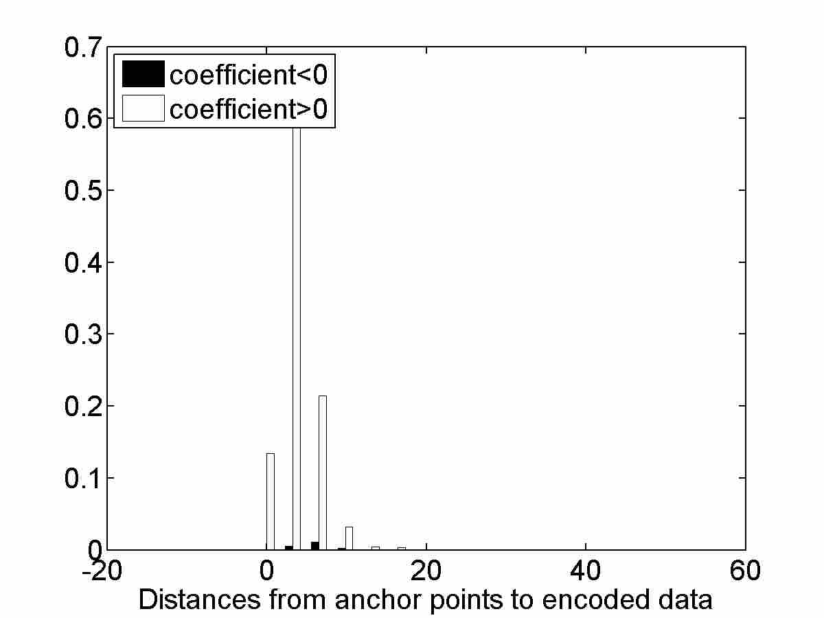
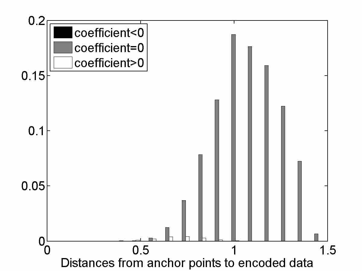
We follow the common experiment setup for Caltech-101, i.e., training on 30 images per category and testing on the rest, and randomly repeat the experiments for 10 times. The step size of the grid is $8$ pixels, and each SIFT is extracted on a $24\times 24$ patch centered at a location; we use $200,000$ random patches’ SIFT descriptors to train the bases for VQ and sparse coding; each image is partitioned into $1\times 1$, $2\times 2$, and $4\times 4$ blocks in 3 different scales, and pooling is done within each of the $21$ blocks. In addition to average pooling, we also try max pooling, i.e., computing the max value of each dimension of codes in each block. Finally the pooled codes are concatenated to form a single image-level feature vector. The results are presented in Table 4. Our methods using sparse coding and local coordinate coding both achieve much higher accuracies on this popular benchmark. Since only linear classifiers are required, the methods are much more scalable and efficient for training and testing, compared to those state-of-the-art methods relying on nonlinear SVMs. We note that local coordinate coding does not produce better results than sparse coding in this experiments. This is because sparse coding in this case is already sufficiently local, as illustrated in Figure 5. This result again is consistent with the main point of the paper, that is, coding locality is essential (and sufficient) for ensuring a good nonlinear learning performance.

Table 4: Classification rate (%) comparison on Caltech-101.

Methods	Accuracy
VQ coding, average pooling, linear SVM	$58.81\pm 1.51$
VQ coding, average pooling, nonlinear SVM	$63.99\pm 0.88$
Sparse coding, average pooling, linear SVM	${66.68\pm 0.66}$
Sparse coding, max pooling, linear SVM	${73.20\pm 0.54}$
Local coordinate coding, average pooling, linear SVM	${66.72\pm 0.52}$
Local coordinate coding, max pooling, linear SVM	${73.14\pm 0.48}$

(a-1)	(a-2)
(b-1)	(b-2)

Figure 5: Coding locality on Caltech-101: (a) sparse coding vs. (b) local coordinate coding.

7 Conclusion

This paper introduces a new method for high dimensional nonlinear learning with data distributed on manifolds. The method can be seen as generalized local linear function approximation, but can be achieved by learning a global linear function with respect to coordinates from unsupervised local coordinate coding. Compared to popular manifold learning methods, our approach can naturally handle unseen data and has a linear complexity with respect to data size. The work also generalizes popular VQ coding and sparse coding schemes, and reveals that locality of coding is essential for supervised function learning. The generalization performance obtained in the paper depends on intrinsic dimensionality of the data manifold. The experiments on synthetic data, handwritten digit data, and object-class images further confirm the findings of our analysis.

While some results in the paper explicitly rely on the manifold concept, the main idea is more general than manifold learning. The theory is valid even when the data do not lie on a manifold. In fact, the manifold structure is only used to bound the complexity of the local coordinate coding scheme, while the general theory can still be applied if we estimate the complexity using other means.

Finally, it is worth mentioning that on many real data, sparse coding (without locality constraint) automatically produces coding schemes that are nearly local. This explains the practical success of sparse coding. It remains an interesting question to investigate conditions under which sparse codes are local, since such conditions directly imply the effectiveness of sparse coding according to our theory.

8 Proofs

8.1 Proof of Proposition 2.1

Consider a change of the ${\mathbb{R}}^{d}$ origin by $u\in{\mathbb{R}}^{d}$, which shifts any point $x\in{\mathbb{R}}^{d}$ to $x+u$, and points $v\in C$ to $v+u$. The shift-invariance requirement implies that after the change, we map $x+u$ to $\sum_{v\in C}\gamma_{v}(x)v+u$, which should equal $\sum_{v\in C}\gamma_{v}(x)(v+u)$. This is equivalent to $u=\sum_{v\in C}\gamma_{v}(x)u$, which holds if and only if $\sum_{v\in C}\gamma_{v}(x)=1$.

8.2 Proof of Lemma 2.1

For simplicity, let $\gamma_{v}=\gamma_{v}(x)$ and $x^{\prime}=\gamma(x)=\sum_{v\in C}\gamma_{v}v$. We have

$$|f(x)-\sum_{v\in C}\gamma_{v}f(v)|$$

$$\leq |f(x)-f(x^{\prime})|+\left|\sum_{v\in C}\gamma_{v}(f(v)-f(x^{\prime}))\right|$$

$$= |f(x)-f(x^{\prime})|+\left|\sum_{v\in C}\gamma_{v}(f(v)-f(x^{\prime})-\nabla f(x^{\prime})^{\top}(v-x^{\prime}))\right|$$

$$\leq |f(x)-f(x^{\prime})|+\sum_{v\in C}|\gamma_{v}||(f(v)-f(x^{\prime})-\nabla f(x^{\prime})^{\top}(v-x^{\prime}))|$$

$$\leq \alpha\|x-x^{\prime}\|_{2}+\beta\sum_{v\in C}|\gamma_{v}|\|x^{\prime}-v\|^{1+p}.$$

This implies the bound.

8.3 Proof of Theorem 2.1

Given any $\epsilon>0$, consider an $\epsilon$-cover $C^{\prime}$ of ${\cal M}$ with $|C^{\prime}|\leq{\cal N}(\epsilon,{\cal M})$. Given each $u\in C^{\prime}$, define $C_{u}=\{v_{1}(u),\ldots,v_{d}(u)\}$, where $v_{j}(u)$ are defined in Definition 2.4. Define the anchor points as

$$C=\cup_{u\in C^{\prime}}\{u+v_{j}(u):j=1,\ldots,m\}\cup C^{\prime}.$$

It follows that $|C|\leq(1+m){\cal N}(\epsilon,{\cal M})$.

In the following, we only need to prove the existence of a coding $\gamma$ on ${\cal M}$ that satisfies the requirement of the theorem. Without loss of generality, we assume that $\|v_{j}(u)\|=\epsilon$ for each $u$ and $j$, and given $u$, $\{v_{j}(u):j=1,\ldots,m\}$ are orthogonal with respect to $A$: $v_{j}^{\top}(u)Av_{k}(u)=0$ when $j\neq k$.

For each $x\in{\cal M}$, let $u_{x}\in C^{\prime}$ be the closest point to $x$ in $C^{\prime}$. We have $\|x-u_{x}\|\leq\epsilon$ by the definition of $C^{\prime}$. Now, Definition 2.4 implies that there exists $\gamma_{j}^{\prime}(x)$ ($j=1,\ldots,m$) such that

$$\left\|x-u_{x}-\sum_{j=1}^{m}\gamma_{j}^{\prime}(x)v_{j}(u_{x})\right\|\leq c_{p}({\cal M})\epsilon^{1+p}.$$

The optimal choice is the $A$-projection of $x-u_{x}$ to the subspace spanned by $\{v_{j}(u_{x}):j=1,\ldots,m\}$. The orthogonality condition thus implies that

$$\sum_{j=1}^{m}\gamma_{j}^{\prime}(x)^{2}\|v_{j}(u_{x})\|^{2}\leq\|x-u_{x}\|^{2}\leq\epsilon^{2}.$$

Therefore

$$\sum_{j=1}^{m}\gamma_{j}^{\prime}(x)^{2}\leq 1,$$

which implies that for all $x$:

$$\sum_{j=1}^{m}|\gamma_{j}^{\prime}(x)|\leq\sqrt{m}.$$

We can now define the coordinate coding of $x\in{\cal M}$ as

$$\gamma_{v}(x)=\left\{\begin{array}[]{cc}\gamma_{j}^{\prime}(x)&v=u_{x}+v_{j}(u_{x})\\ 1-\sum_{j=1}^{m}\gamma_{j}^{\prime}(x)&v=u_{x}\\ 0&\text{otherwise}\end{array}\right..$$

This implies the following bounds:

$$\|x-\gamma(x)\|\leq c_{p}({\cal M})\epsilon^{1+p}$$

and

$$\sum_{v\in C}\gamma_{v}(x)\left\|v-\gamma(x)\right\|^{1+p}$$

$$= |\gamma_{u_{x}}(x)|\|\gamma(x)-u_{x}\|^{1+p}+\sum_{j=1}^{m}|\gamma_{j}^{\prime}(x)|\left\|v_{j}(u_{x})-(\gamma(x)-u_{x})\right\|^{1+p}$$

$$\leq (1+\sqrt{m})\epsilon^{1+p}+\sum_{j=1}^{m}|\gamma_{j}^{\prime}(x)|(\epsilon+\epsilon)^{1+p}$$

$$= [1+\sqrt{m}+2^{1+p}\sqrt{m}]\epsilon^{1+p},$$

where we have used $\|v-u_{x}\|=\epsilon$, and $\|\gamma(x)-u_{x}\|\leq\|x-u_{x}\|\leq\epsilon$ (note that $\gamma(x)-u_{x}$ is the projection of $x-u_{x}$).

8.4 Proof of Theorem 3.1

Consider $n+1$ samples $S_{n+1}=\{(x_{1},y_{1}),\ldots,(x_{n+1},y_{n+1})\}$. We shall introduce the following notation:

$$[\tilde{w}_{v}]=\arg\min_{[w_{v}]}\left[\frac{1}{n}\sum_{i=1}^{n+1}\phi\left(f_{\gamma,C}(w,x_{i}),y_{i}\right)+\lambda\sum_{v\in C}w_{v}^{2}\right].$$ (5)

Let $k$ be an integer randomly drawn from $\{1,\ldots,n+1\}$. Let $[\hat{w}^{(k)}_{v}]$ be the solution of

$$[\hat{w}_{v}^{(k)}]=\arg\min_{[w_{v}]}\left[\frac{1}{n}\sum_{i=1,\ldots,n+1;i\neq k}\phi\left(f_{\gamma,C}(w,x_{i}),y_{i}\right)+\lambda\sum_{v\in C}w_{v}^{2}\right],$$

with the $k$-th example left-out.

We have the following stability lemma from [8], which can be stated as follows using our terminology:

Lemma 8.1

The following inequality holds

$$|f_{\gamma,C}(\hat{w}^{(k)},x_{k})-f_{\gamma,C}(\tilde{w},x_{k})|\leq\frac{\|x_{k}\|_{\gamma}^{2}}{2\lambda n}|\phi_{1}^{\prime}(f_{\gamma,C}(\tilde{w},x_{k}),y_{k})|.$$

By using Lemma 8.1, we obtain for all $\alpha>0$:

$$\phi(f_{\gamma,C}(\tilde{w},x_{k}),y_{k})-\phi(f_{\gamma,C}(\hat{w}^{(k)},x_{k}),y_{k})$$

$$= \phi(f_{\gamma,C}(\tilde{w},x_{k}),y_{k})-\phi(f_{\gamma,C}(\hat{w}^{(k)},x_{k}),y_{k})$$

$$\quad-\phi_{1}^{\prime}(f_{\gamma,C}(\hat{w}^{(k)},x_{k}),y_{k})(f_{\gamma,C}(\tilde{w},x_{k})-f_{\gamma,C}(\hat{w}^{(k)},x_{k}))$$

$$\quad+\phi_{1}^{\prime}(f_{\gamma,C}(\hat{w}^{(k)},x_{k}),y_{k})(f_{\gamma,C}(\tilde{w},x_{k})-f_{\gamma,C}(\hat{w}^{(k)},x_{k}))$$

$$\geq \phi_{1}^{\prime}(f_{\gamma,C}(\hat{w}^{(k)},x_{k}),y_{k})(f_{\gamma,C}(\tilde{w},x_{k})-f_{\gamma,C}(\hat{w}^{(k)},x_{k}))$$

$$\geq -\phi_{1}^{\prime}(f_{\gamma,C}(\hat{w}^{(k)},x_{k}),y_{k})^{2}\|x_{k}\|_{\gamma}^{2}/(2\lambda n)$$

$$\geq -B^{2}\|x_{k}\|_{\gamma}^{2}/(2\lambda n).$$

In the above derivation, the first inequality uses the convexity of $\phi(f,y)$ with respect to $f$, which implies that $\phi(f_{1},y)-\phi(f_{2},y)-\phi_{1}^{\prime}(f_{2},y)(f_{1}-f_{2})\geq 0$. The second inequality uses Lemma 8.1, and the third inequality uses the assumption of the loss function.

Now by summing over $k$, and consider any fixed $f\in{\cal F}_{\alpha,\beta,p}$, we obtain:

$$\sum_{k=1}^{n+1}\phi(f_{\gamma,C}(\hat{w}^{(k)},x_{k}),y_{k})$$

$$\leq \sum_{k=1}^{n+1}\left[\phi(f_{\gamma,C}(\tilde{w},x_{k}),y_{k})+\frac{B^{2}}{2\lambda n}\|x_{k}\|_{\gamma}^{2}\right]$$

$$\leq n\left[\frac{1}{n}\sum_{k=1}^{n+1}\phi\left(\sum_{v\in C}\gamma_{v}(x_{k})f(v),y_{k}\right)+\lambda\sum_{v\in C}f(v)^{2}\right]+\frac{B^{2}}{2\lambda n}\sum_{k=1}^{n+1}\|x_{k}\|_{\gamma}^{2}$$

$$\leq n\left[\frac{1}{n}\sum_{k=1}^{n+1}[\phi\left(f(x_{k}),y_{k}\right)+BQ(x_{k})]+\lambda\sum_{v\in C}f(v)^{2}\right]+\frac{B^{2}}{2\lambda n}\sum_{k=1}^{n+1}\|x_{k}\|_{\gamma}^{2},$$

where $Q(x)=\alpha\left\|x-\gamma(x)\right\|+\beta\sum_{v\in C}|\gamma_{v}(x)|\left\|v-\gamma(x)\right\|^{1+p}$. In the above derivation, the second inequality follows from the definition of $\tilde{w}$ as the minimizer of (5). The third inequality follows from Lemma 2.1. Now by taking expectation with respect to $S_{n+1}$, we obtain

$$(n+1){\mathbb{E}}_{S_{n+1}}\phi(f_{\gamma,C}(\hat{w}^{(n+1)},x_{n+1}),y_{n+1})$$

$$\leq n\left[\frac{n+1}{n}{\mathbb{E}}_{x,y}\phi\left(f(x),y\right)+\frac{n+1}{n}BQ_{\alpha,\beta,p}(\gamma,C)+\lambda\sum_{v\in C}f(v)^{2}\right]+\frac{B^{2}(n+1)}{2\lambda n}{\mathbb{E}}_{x}\|x\|_{\gamma}^{2}.$$

This implies the desired bound.

8.5 Proof of Theorem 3.2

Note that any measurable function $f:{\cal M}\to R$ can be approximated by ${\cal F}_{\alpha,\beta,p}$ with $\alpha,\beta\to\infty$ and $p=0$. Therefore we only need to show

$$\lim_{n\to\infty}{\mathbb{E}}_{S_{n}}\;{\mathbb{E}}_{x,y}\phi(f_{\gamma,C}(\hat{w},x),y)=\lim_{n\to\infty}\inf_{f\in{\cal F}_{\alpha,\beta,p}}{\mathbb{E}}_{x,y}\phi\left(f(x),y\right).$$

Theorem 2.1 implies that it is possible to pick $(\gamma,C)$ such that $|C|/n\to 0$ and $Q_{\alpha,\beta,p}(\gamma,C)\to 0$. Moreover, $\|x\|_{\gamma}$ is bounded.

Given any $f\in{\cal F}_{\alpha,\beta,0}$ and any constant $A>0$ that is independent of $n$; if we let $f_{A}(x)=\max(\min(f(x),A),-A)$, then it is clear that $f_{A}(x)\in{\cal F}_{\alpha,\alpha+\beta,0}$. Therefore Theorem 3.1 implies that as $n\to\infty$,

$${\mathbb{E}}_{S_{n}}\;{\mathbb{E}}_{x,y}\phi(f_{\gamma,C}(\hat{w},x),y)\leq{\mathbb{E}}_{x,y}\phi\left(f_{A}(x),y\right)+o(1).$$

Since $A$ is arbitrary, we let $A\to\infty$ to obtain the desired result.

References

- [1] Mikhail Belkin and Partha Niyogi. Laplacian eigenmaps for dimensionality reduction and data representation. Neural Comput., 15(6):1373–1396, 2003.
- [2] G. E. Hinton and R. R. Salakhutdinov. Reducing the dimensionality of data with neural networks. Science, 313(5786):504 – 507, July 2006.
- [3] S. Lazebnik, C. Schmid, and J. Ponce. Beyond bags of features: Spatial pyramid matching for recognizing natural scene categories. IEEE Conference on Computer Vision and Pattern Recognition, 2006.
- [4] Rajat Raina, Alexis Battle, Honglak Lee, Benjamin Packer, and Andrew Y. Ng. Self-taught learning: Transfer learning from unlabeled data. International Conference on Machine Learning, 2007.
- [5] Sam Roweis and Lawrence Saul. Nonlinear dimensionality reduction by locally linear embedding. Science, 290(5500):2323–2326, 2000.
- [6] J. B. Tenenbaum, V. De Silva, and J. C. Langford. A global geometric framework for nonlinear dimensionality reduction. Science, 290(5500):2319–2323, 2000.
- [7] Alon Zakai and Ya’acov Ritov. Consistency and localizability. Journal of Machine Learning Research, 10:827–856, 2009.
- [8] Tong Zhang. Leave-one-out bounds for kernel methods. Neural Computation, 15:1397–1437, 2003.