Information Accessibility and Cryptic Processes:
Linear Combinations of Causal States

Abstract

We show in detail how to determine the time-reversed representation of a stationary hidden stochastic process from linear combinations of its forward-time $\epsilon$-machine causal states. This also gives a check for the $k$-cryptic expansion recently introduced to explore the temporal range over which internal state information is spread.

I Introduction

We introduced a new system “invariant”—the crypticity $\chi$—for stationary hidden stochastic processes to capture how much internal state information is directly accessible (or not) from observations [1, 2, 3]. Two approaches to calculate $\chi$ were given. The first, reported in Ref. [1] and Ref. [2], used the so-called mixed-state method, which employs linear combinations of a process’s forward-time $\epsilon$-machine. The second, appearing in Ref. [3], developed a systematic expansion $\chi(k)$ as a function of the length $k$ of observed sequences over which internal state information can be extracted. The mixed-state method is the most efficient way to calculate crypticity and other important system properties, such as the excess entropy ${\bf E}$, since it avoids having to write out all of the terms required for calculating $\chi(k)$. It also does not rely on knowing in advance a process’s cryptic order.

As such, we reported results in Ref. [3] that use the mixed-state method to, in a sense, calibrate the $\chi(k)$ expansion and to understand its convergence.

Here we provide the calculational details behind those results. Generally, though, the goal is to find out what a stochastic process looks like when scanned in the “opposite” time direction. Specifically, starting with a given $\epsilon$-machine $M$ of a process, calculate its reverse-time representation $M^{-}$. (The latter is not always minimal and so not, in that case, an $\epsilon$-machine.) This is done in two steps: (i) time-reverse $M$, producing $\widehat{M}=\mathcal{T}(M)$, and (ii) convert $\widehat{M}$ to a unifilar presentation $\mathcal{U}(\widehat{M})$ using mixed states, which are linear combinations of the states of $\widehat{M}$.

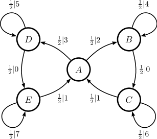
Figure 1: A $2$-cryptic process: The $\epsilon$-machine representation of the Butterfly Process. Edge labels $t|{x}$ give the probability $t=T^{({x})}_{\sigma\sigma^{\prime}}$ of making a transition and from causal state $\sigma$ to causal state $\sigma^{\prime}$ and seeing symbol ${x}$.

In the following, we show how to implement these steps for the various example processes presented in Ref. [3]: the Butterfly, Restricted Golden Mean, and Nemo Processes. We jump directly into the calculations, assuming the reader is familiar with Refs. [1], [2], and [3]. Those references provide, in addition, more discussion and motivation and reasonable list of citations.

II Butterfly Process

Figure 1 shows the $\epsilon$-machine for Ref. [3]’s Butterfly process—an output process over eight symbols $\mathcal{A}=\{0,1,\ldots,7\}$.

Since its transition matrices are doubly stochastic, the stationary state distribution is uniform. This immediately gives its stored information: the statistical complexity is $C_{\mu}=\log_{2}(5)$ bits. It also makes the construction of the time-reverse machine straightforward: We simply reverse the directions of all the arrows. (See Fig. 2.) Note that the time-reverse presentation is no longer unifilar and, therefore, it is not the reversed process’s $\epsilon$-machine.

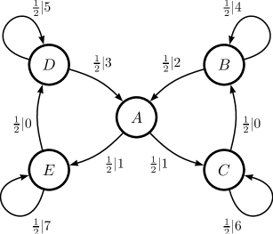
Figure 2: Time-reversed Butterfly Process.

Due to this we must calculate the mixed-state presentation to find a unifilar presentation. The calculated mixed states and the words which induce them are given in Table 1.

Allowed Words	$\mu$ or Previous Word
0	(0,$\frac{1}{2}$,0,$\frac{1}{2}$,0)
1	(0,0,$\frac{1}{2}$,0,$\frac{1}{2}$)
2	(1,0,0,0,0)
3	2
4	(0,1,0,0,0)
5	(0,0,0,1,0)
6	(0,0,1,0,0)
7	(0,0,0,0,1)
02	2
03	2
04	4
05	5
10	0
16	6
17	7
21	1
42	2
44	4
53	2
55	5
60	4
66	6
70	5
77	7

Table 1: Calculating the time-reversed Butterfly Process’s $\epsilon$-machine via the forward $\epsilon$-machine’s mixed states. The $5$-vector denotes the mixed-state distribution $\mu(w)$ reached after having seen the corresponding allowed word $w$. If the word leads to a unique state with probability one, we give instead the state’s name.

The result is the reverse $\epsilon$-machine shown in Fig. 3. Note that it has two more states than the original (forward) $\epsilon$-machine of Fig. 1.

The stationary distribution of this reversed machine is $\pi=(0.1,0.2,0.2,0.15,0.15,0.1,0.1)$. Now we are in position to calculate ${\bf E}$ using the result of Ref. [1]:

$${\bf E} =C_{\mu}-\chi$$ (1)

$${\bf E} =C_{\mu}-H[{\mathcal{S}}^{+}|\overrightarrow{{X}}]$$ (2)

$$=C_{\mu}-H[{\mathcal{S}}^{+}|{\mathcal{S}}^{-}=\epsilon^{+}(\overrightarrow{{X}})]~{}.$$ (3)

In this case, we find a crypticity of:

$$\chi =H[{\mathcal{S}}^{+}|{\mathcal{S}}^{-}]$$

$$=0.1H[(0,\frac{1}{2},0,\frac{1}{2},0)]+0.2H[(0,0,\frac{1}{2},0,\frac{1}{2})]$$

$$\quad+0.2H[(1,0,0,0,0)]+0.15H[(0,1,0,0,0)]$$

$$\quad+0.15H[(0,0,0,1,0)]+0.1H[(0,0,1,0,0)]$$

$$\quad+0.1H[(0,0,0,0,1)]$$

$$=0.1+0.2$$

$$=0.3~{}\mathrm{bits}.$$

So, ${\bf E}=\log_{2}(5)-0.3\approx 2.0219$ bits, in accord with the result calculated via Thm. 1 of Ref. [3].

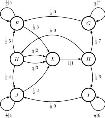
Figure 3: Reverse Butterfly Process.

III Restricted Golden Mean Process

For reference, we give the family of labeled transition matrices for the binary Restricted Golden Mean Process (RGMP):

$$T^{(0)} =\begin{pmatrix}0&\frac{1}{2}&0&0&0&\cdots\\ 0&0&0&0&0&\cdots\\ 0&0&0&0&0&\cdots\\ 0&0&0&0&0&\cdots\\ \vdots&\vdots&\vdots&\vdots&\vdots&\ddots\\ 0&0&0&0&0&\cdots\end{pmatrix}$$

and

$$T^{(1)} =\begin{pmatrix}\frac{1}{2}&0&0&0&0&\cdots\\ 0&0&1&0&0&\cdots\\ 0&0&0&1&0&\cdots\\ 0&0&0&0&1&\cdots\\ \vdots&\vdots&\vdots&\vdots&\vdots&\ddots\\ 1&0&0&0&0&\cdots\end{pmatrix}~{}.$$

Its $\epsilon$-machine is given in Fig. 4 and its stationary distribution is:

$$\pi=\left(\frac{2}{k+2},\frac{1}{k+2},\frac{1}{k+2},\ldots,\frac{1}{k+2}\right)~{}.$$

Figure 4: The $\epsilon$-machine for the Restricted Golden Mean Process.

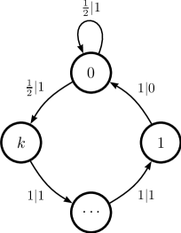
Figure 5: Time-reversed presentation of the Restricted Golden Mean Process.

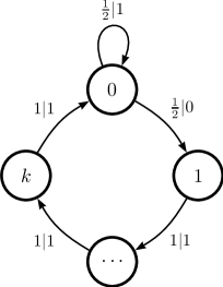
Figure 6: Reverse Restricted Golden Mean Process.

Allowed Words	$\mu$ or Previous Word
0	$(1,0^{k})$
1	$(\frac{1}{k+1},\frac{1}{k+1},\ldots,\frac{1}{k+1})$
01	$(\frac{1}{2},0^{k-1},\frac{1}{2})$
10	0
11	$\frac{1}{k}(\frac{1}{2},1,1,\ldots,1,\frac{1}{2})$
⋮	⋮
0$(1)^{n}$ for $1\leq n\leq k$	$(\frac{1}{2^{n}},0^{k-n},\frac{1}{2^{1}}\frac{1}{2^{2}}\frac{1}{2^{3}},\ldots,\frac{1}{2^{n}})$
1$(1)^{n}$ for $1\leq n\leq k$	$\frac{1}{k-n+1}(\frac{1}{2^{n}},1^{k-n},\frac{1}{2^{1}}\frac{1}{2^{2}}\frac{1}{2^{3}},\ldots,\frac{1}{2^{n}})$
0$(1)^{k}$	$(\frac{1}{2^{k}},\frac{1}{2^{1}}\frac{1}{2^{2}}\frac{1}{2^{3}},\ldots,\frac{1}{2^{k}})$
1$(1)^{k}$	0$(1)^{k}$
0$(1)^{k}$0	0
0$(1)^{k}$1	0$(1)^{k}$

Table 2: Calculating the reversed RGMP using mixed states over the $\epsilon$-machine states.

Through other methods, we can show that the RGMP is reversible. We “push” RGMP to an edge machine presentation and “pull” $\mathcal{T}$(RGMP) also the same type of presentation. (An edge machine presentation of a machine $M$ has states that are the edges of $M$.) These machines are the same. Therefore, the forward and reverse $\epsilon$-machines are the same and, moreover, we can use the same mixed-state inducing word list. It is easy to see that one such list is $(0,01,011,\ldots,01^{k})$. Table 2 gives the mixed states for these allowed words. It is also reasonably clear from the above mixed-state presentation that these correspond to the recurrent causal states for the time-reversed process’s $\epsilon$-machine.

With this, we can now compute $\chi$ using $H[{\mathcal{S}}^{+}|{\mathcal{S}}^{-}]$, as follows:

$$H[{\mathcal{S}}^{+}|{\mathcal{S}}^{-}=0] =H[(1,0^{k})]=0~{}\mathrm{and}$$

$$H[{\mathcal{S}}^{+}|{\mathcal{S}}^{-}=0(1)^{n}] =H[(\frac{1}{2^{n}},0^{k-n},\frac{1}{2^{1}}\frac{1}{2^{2}}\frac{1}{2^{3}},\ldots,\frac{1}{2^{n}})]~{}.$$

So that, in general, we have:

$$H[{\mathcal{S}}^{+}|{\mathcal{S}}^{-}] =\sum_{n=1}^{k-1}{\frac{1}{k+2}H[(\frac{1}{2^{n}},0^{k-n},\frac{1}{2^{1}}\frac{1}{2^{2}}\frac{1}{2^{3}},\ldots,\frac{1}{2^{n}})]}$$

$$\quad+\frac{2}{2+k}H[(\frac{1}{2^{k}},\frac{1}{2^{1}}\frac{1}{2^{2}}\frac{1}{2^{3}},\ldots,\frac{1}{2^{k}})]~{}.$$

It can then be shown that:

$$H[(\frac{1}{2^{n}} ,0^{k-n},\frac{1}{2^{1}}\frac{1}{2^{2}}\frac{1}{2^{3}},\ldots,\frac{1}{2^{n}})]$$

$$=H[(\frac{1}{2^{n}},\frac{1}{2^{1}}\frac{1}{2^{2}}\frac{1}{2^{3}},\ldots,\frac{1}{2^{n}})]$$

$$=2-2^{(1-n)}~{}.$$

Therefore, returning to the causal-state-conditional entropy of interest, we have:

$$H[{\mathcal{S}}^{+}|{\mathcal{S}}^{-}] =\frac{1}{k+2}\sum_{n=1}^{k-1}{(2-2^{(1-n)})}+\frac{2}{2+k}(2-2^{(1-k)})$$

$$=\frac{1}{k+2}(2(k-1)+2(2-2^{1-k})-(2-2^{2-k}))$$

$$=\frac{2k}{k+2}~{}.$$

With a few more steps, we arrive at our destination—the RGMP’s informational quantities:

$$C_{\mu} =\log 2(k+2)-\frac{2}{k+2}~{},$$

$$\chi =\frac{2k}{k+2},~{}\mathrm{and}$$

$${\bf E} =\log 2(k+2)-\frac{2(k+1)}{k+2}~{}.$$

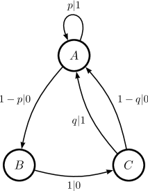
Figure 7: The $\epsilon$-machine for the $\infty$-cryptic Nemo Process.

IV Nemo Process

We now demonstrate how to calculate $\chi$ and ${\bf E}$ for Ref. [3]’s $\infty$-cryptic process—the Nemo Process—using mixed-state methods. As emphasized in Ref. [3], the $k$-cryptic expansion there cannot be applied in this case. Thus, the Nemo Process demonstrates that Refs. [1] and [2]’s mixed-state method is essential.

Figure 7 shows ${M}^{+}$, the $\epsilon$-machine for the forward-scanned Nemo Process. Its transition matrices are:

$$T^{(0)} =\bordermatrix{&A&B&C\cr A&0&1-p&0\cr B&0&0&1\cr C&1-q&0&0}\textrm{ and }$$

$$T^{(1)} =\bordermatrix{&A&B&C\cr A&p&0&0\cr B&0&0&0\cr C&q&0&0}.$$

The stationary state distribution is the normalized left-eigenvector of $T\equiv T^{(0)}+T^{(1)}$ and is given by:

$$\Pr({\mathcal{S}}^{+})\equiv\pi^{+}=\frac{1}{3-2p}\bordermatrix{&A&B&C\cr&1&1-p&1-p}.$$

Then, the statistical complexity is the Shannon entropy over these states:

$$C_{\mu} =H[{\mathcal{S}}^{+}]$$

$$=\log_{2}(3-2p)-\frac{2(1-p)}{3-2p}\log_{2}(1-p)~{}.$$

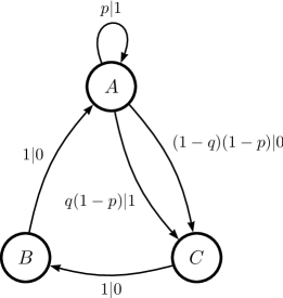
Figure 8: The time-reversed presentation, $\widetilde{M}^{+}=\mathcal{T}({M}^{+})$, of the Nemo Process.

The next step is to construct the time-reversed presentation $\widetilde{M}^{+}=\mathcal{T}({M}^{+})$, shown in Fig. 8. The transition matrices of this machine are:

$$\widetilde{T}^{(0)} =\bordermatrix{&A&B&C\cr A&0&0&(1-q)(1-p)\cr B&1&0&0\cr C&0&1&0\cr}\textrm{ and}$$

$$\widetilde{T}^{(1)} =\bordermatrix{&A&B&C\cr A&p&0&q(1-p)\cr B&0&0&0\cr C&0&0&0\cr}.$$

Finally, we construct the mixed-state presentation of the time-reversed presentation, $\mathcal{U}(\widetilde{M}^{+})$, which is shown in Fig. 9. On doing so, we obtain the following mixed states:

$$D\equiv\nu(1) =\frac{1}{p+q-pq}\bordermatrix{&A&B&C\cr&p&0&q(1-p)}~{},$$

$$E\equiv\nu(01) =\frac{1}{p+q-pq}\bordermatrix{&A&B&C\cr&0&q&p(1-q)}~{},~{}\mathrm{and}$$

$$F\equiv\nu(001) =\frac{1}{p+q-pq}\bordermatrix{&A&B&C\cr&q&p(1-q)&0}~{}.$$

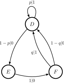
Figure 9: The reverse $\epsilon$-machine for the Nemo Process.

These mixed states form the reverse $\epsilon$-machine causal states, which are exactly the same as the forward $\epsilon$-machine. Thus, the Nemo Process is causally reversible. The mixed states are distributions giving the probabilities of the forward causal states conditioned on a reverse causal state:

$$\Pr({\mathcal{S}}^{+}|{\mathcal{S}}^{-}) =\frac{1}{p+q-pq}\bordermatrix{&A&B&C\cr D&p&0&q(1-p)\cr E&0&q&p(1-q)\cr F&q&p(1-q)&0\cr}~{}.$$

We use this to directly compute:

$$H[{\mathcal{S}}^{+}|{\mathcal{S}}^{-}] =\frac{1}{3-2p}\biggl{[}\frac{p}{p+q-pq}\log_{2}\left(\frac{p+q-pq}{p}\right)\biggl{.}$$

$$\quad\biggl{.}+\frac{q(1-p)}{p+q-pq}\log_{2}\left(\frac{p+q-pq}{q(1-p)}\right)\biggr{]}$$

$$\quad+\frac{2(1-p)}{3-2p}\biggl{[}\frac{q}{p+q-pq}\log_{2}\left(\frac{p+q-pq}{q}\right)\biggr{.}$$

$$\quad\biggl{.}+\frac{p(1-q)}{p+q-pq}\log_{2}\left(\frac{p+q-pq}{p(1-q)}\right)\biggr{]}~{}.$$

Finally, we have:

$${\bf E} =C_{\mu}-H[{\mathcal{S}}^{+}|{\mathcal{S}}^{-}]$$

$$=\log_{2}(3-2p)-\frac{2(1-p)}{3-2p}\log_{2}(1-p)$$

$$\quad-\frac{1}{3-2p}\biggl{[}\frac{p}{p+q-pq}\log_{2}\left(\frac{p+q-pq}{p}\right)\biggl{.}$$

$$\quad\biggl{.}+\frac{q(1-p)}{p+q-pq}\log_{2}\left(\frac{p+q-pq}{q(1-p)}\right)\biggr{]}$$

$$\quad+\frac{2(1-p)}{3-2p}\biggl{[}\frac{q}{p+q-pq}\log_{2}\left(\frac{p+q-pq}{q}\right)\biggr{.}$$

$$\quad\biggl{.}+\frac{p(1-q)}{p+q-pq}\log_{2}\left(\frac{p+q-pq}{p(1-q)}\right)\biggr{]}~{}.$$

V Conclusion

The detailed calculations make evident that Refs. [1] and [2]’s mixed-state method gives a new level of direct analysis for the informational properties of stationary stochastic processes, such as the crypticity and the excess entropy. The complementary approach given by the crypticity expansion $\chi(k)$ is useful in understanding information accessibility—how internal state information is spread over time in measurement sequences [3]. Nonetheless, while $\chi(k)$ can be calculated in particular finite cases, the mixed-state method is the most general and efficient method.

References

[1]
J. P. Crutchfield, C. J. Ellison, and J. Mahoney.
Time’s barbed arrow: Irreversibility, crypticity, and stored
information.
submitted, 2009.
arxiv.org:0902.1209 [cond-mat].
[2]
C. J. Ellison, J. R. Mahoney, and J. P. Crutchfield.
Prediction, retrodiction, and the amount of information stored in the
present.
arxiv: 0905.3587 [cond-mat], 2009.
[3]
J. R. Mahoney, C. J. Ellison, , and J. P. Crutchfield.
Information accessibility and cryptic processes.
submitted, 2009.
arxiv.org:0905.4787 [cond-mat].