Using the $\Delta_{3}$ statistic to test for missed levels in mixed sequence neutron resonance data.

Abstract

The $\Delta_{3}(L)$ statistic is studied as a tool to detect missing levels in the neutron resonance data where 2 sequences are present. These systems are problematic because there is no level repulsion, and the resonances can be too close to resolve. $\Delta_{3}(L)$ is a measure of the fluctuations in the number of levels in an interval of length $L$ on the energy axis. The method used is tested on ensembles of mixed Gaussian Orthogonal Ensemble (GOE) spectra, with a known fraction of levels ($x\%$) randomly depleted, and can accurately return $x$. The accuracy of the method as a function of spectrum size is established. The method is used on neutron resonance data for 11 isotopes with either s-wave neutrons on odd-A, or p-wave neutrons on even-A. The method compares favorably with a maximum likelihood method applied to the level spacing distribution. Nuclear Data Ensembles were made from 20 isotopes in total, and their $\Delta_{3}(L)$ statistic are discussed in the context of Random Matrix Theory.

I Introduction

Neutron resonance data provides us with a list of eigenvalues of the nuclear Hamiltonian. As such, they are a testing ground for a range of ideas in theoretical nuclear physics, from level density models to quantum chaos Weidenmüller and Mitchell (2009); Guhr et al. (1998). The data sets are rarely complete, levels are invariably missed, due to the finite resolution of the experimental apparatus, or the weakness of the signal, or some other factor. Whatever the reason for levels being missed, it is important to have an estimate of how incomplete a data set is. When the data is a mixture of 2 sequences of levels (a sequence of levels is a set of levels with the same quantum number), there is no level repulsion, levels can be very close indeed, and the number of missed levels is expected to increase. We can use Random Matrix Theory (RMT) to estimate the number of missed levels. An analysis based on RMT works because at the excitation energies involved, $\approx 7$ MeV, the nucleus is a chaotic system and the nuclear spectra have the same fluctuation properties as the Gaussian Orthogonal Ensembles (GOE) Brody et al. (1981); Stockmann (1999); Bohigas et al. (1984). Various statistics of RMT have been used to evaluate the completeness of data in the past Brody et al. (1981). The most popular statistic is the level spacing distribution, $P(s)$. The $\Delta_{3}(L)$ statistic, introduced by Dyson Dyson and Mehta (1963) has traditionally been underexploited for this task. The sensitivity of the $\Delta_{3}(L)$ statistic was reevaluated in Mulhall et al. (2007), where it was shown that the actual variance of the $\Delta_{3}(L)$ statistic calculated from a specific spectrum was smaller than the ensemble result. It was then used for statistical spectroscopy to give information on missed levels in a single sequence of pure neutron resonance data. The situation is more complicated, however when the data consists of 2 sequences of levels. In this case the quantum number that differs between the sequences is spin. When s-wave neutrons (angular momentum $L=0$) are incident on an odd-A isotope, with spin-$j$, the neutron resonances have two possible spin values, $j\pm\frac{1}{2}$. When p-wave neutrons (angular momentum $L=1$) are incident on an even-even (spin-zero) isotope, the possible spin values for the resonances are $\frac{1}{2}$ or $\frac{3}{2}$. The level repulsion that is present in single sequence data is gone, and now levels can be very close indeed. This makes them easier to miss by counting two separate levels as one, and the number of missed levels may increase.

In this work the neutron resonance data of s-wave neutrons incident on 7 odd-A isotopes, and p-wave neutrons on 4 even-even isotopes was analyzed with a RMT method, to gauge the completeness of the data. The $\Delta_{3}(L)$ values for each set of neutron resonance data were compared to the RMT results from a numerical ensemble. There is no closed form expression for the $\Delta_{3}(L)$ statistic for mixed, depleted GOE spectra, so we found it numerically. A range of ensembles of mixed depleted GOE spectra was made. Each ensemble consisted of 500 spectra. Each spectra was a mixture of 2 unfolded GOE spectra, mixed in a proportion $\alpha:(1-\alpha)$, appropriate to the isotope in question. Furthermore the spectrum size, $N$, was appropriate for comparison with the experimental data. Each spectra in an ensemble was depleted by $x$%, by randomly deleting levels. The probability of deletion was uniform across the spectrum i.e. independent of energy. Other energy dependant probability distributions were used, in an attempt to mimic experimental resolution but the results were the same. There were 21 ensembles for each value of $\alpha$ and $N$, one for each value of $x$ from 0% to 10% in steps of 0.5%. A comparison of $\Delta_{3}(L)$ from the experimental spectrum with the appropriate ensembles gave an estimate of $x$. These results were compared with those of a MLM analysis based on $P(s)$.

First, we make a few comments on the basic approach of using random matrices to model real physical systems. Specific nuclear energy levels are incalculable at neutron separation energies. The system is too complex and the level density is too large so that even a weak residual interaction would mix whatever basis states you start with into a random superposition. In other words, the Hamiltonian is, for all practical purposes, random. Given a set of energy levels with the same quantum numbers (a pure sequence) from a complex system, in a region of high level density, the only clue available to the system it came from would be the functional form of the level density itself, this is a so-called secular variation. If you removed this system-specific information by rescaling the energies so that the adjusted spectrum had a uniform level density, and an average spacing of one, then all that would remain of your original spectra are the fluctuation properties. It turns out that these fluctuation properties are rich in information about the system. This rescaling is known as unfolding Guhr et al. (1998); Brody et al. (1981). It is a powerful idea, because it strips away all the details that depend on the specifics of the system. The only surviving features are in the statistical fluctuations of the spectra, and these are due to the global symmetries of the system. These fluctuations are the variables of RMT. It is the purpose of this work to use one of them, $\Delta_{3}(L)$, to estimate the number of levels missed in neutron resonance experiments.

In the next section we describe the $\Delta_{3}(L)$ statistic and give the GOE results for the cases of complete single and mixed spectra. The distinction between spectral and ensemble averages is clarified. The details of the calculation of GOE spectra, the unfolding procedure, and the evaluation of $\Delta_{3}(L)$ are explained. In Sect. III, the method of determining the fraction of levels missing from a spectrum, using both $\Delta_{3}(L)$ and $P(s)$ is explained. Both methods are tested on depleted, mixed GOE spectra. Sect. IV sets of neutron resonance date are themselves grouped into Nuclear Data Ensembles, and a qualitative comparison with the GOE is made. In Sect. V we describe the experimental data sets and discuss the results.

II The $\Delta_{3}(L)$ statistic: definition and calculation

The $\Delta_{3}(L)$ statistic is a robust statistic for a RMT analysis, revealing a remarkable long range correlation in chaotic spectra. It is a measure of the variance in the number of levels in an interval of length $L$ anywhere on the energy axis. It is defined in terms of the cumulative level number, ${\mathcal{N}}(E)$, the number of levels with energy less than or equal to $E$. A graph of ${\mathcal{N}}(E)$ is a staircase function, each step is one unit high, and $s$ units deep, where $s$ is the level spacing. A harmonic oscillator spectrum has no fluctuations, so in this case ${\mathcal{N}}(E)$ will look like stairs at a $45^{\circ}$ angle. In the case of a GOE spectrum, random fluctuations will make ${\mathcal{N}}(E)$ deviate from the regular staircase. The $\Delta_{3}(L)$ statistic measures this deviation. It is defined by:

$$\Delta_{3}(L) = \left\langle{\rm min}_{A,B}\;\frac{1}{L}\;\int^{E_{i}+L}_{E_{i}}dE^{\prime}\,[\;{\mathcal{N}}(E^{\prime})-AE^{\prime}-B]^{2}\;\;\right\rangle$$ (1)

$$= \langle\Delta^{i}_{3}(L)\rangle\>,$$

where we use angle brackets to denote the spectral average of a quantity, in this case, the average is over all values of $i$, the location of the window of $L$ levels within the spectrum. $A$ and $B$ have values that minimize $\Delta^{i}_{3}(L)$; they are recalculated for each value of $i$. In the case of the perfectly rigid harmonic oscillator, the triangles between the staircase ${\mathcal{N}}(E)$, and the straight line, $AE-B$, with $A=1$, $B=0$, will give us $\Delta_{3}(L)=1/12$. At the other extreme, a classically regular system will lead to a quantum mechanical spectrum with no level repulsion, the fluctuations are far greater, and $\Delta_{3}(L)=L/15$. Such a spectrum is referred to as Poissonian. The asymptotic RMT result for the Gaussian Orthogonal Ensemble (GOE) is

$$\Delta_{3}(L) = \frac{1}{\pi^{2}}\,\left[\log(2\pi L)+\gamma-\frac{5}{4}-\frac{\pi^{2}}{8}\right]\;$$ (2)

$$= \frac{1}{\pi^{2}}(\log L-0.0678)\>,$$

with $\gamma$ being Euler’s constant. The ensemble variance of $\Delta_{3}(L)$ is $\sigma_{e}^{2}=(0.110)^{2}$.

The difference between ensemble and spectral averaging is important here, and we need to be very clear on what this means. When there is risk of confusion, we will use an overline for an ensemble average, as opposed to the angle brackets used for spectral averages. If you take a single GOE spectrum, and look at any window of $L$ levels, calculate the quantity inside the angle brackets in Eq. 1, ($i$ will be fixed at some random value), then you have a single number, i.e. $\Delta^{i}_{3}(L)$. Eq. 2 gives the average value of this number evaluated for many different spectra, and the variance of this number is 0.110, independent of the value of $L$. This is an ensemble average. The definition (1) implies a spectral average, but (2) is an ensemble average. The GOE result in Eq. 1 could be written $\overline{\Delta}_{3}(L)$, but traditionally the overline is dropped, as RMT results typically pertain to ensemble averages. The ambiguous notation, while standard, is unfortunate.

The practical job of using the $\Delta_{3}(L)$ statistic to detect missed levels depends on the variance of the statistic. The value $\sigma_{e}^{2}=0.110^{2}$ is too large to be useful, but this is the ensemble result. When analyzing a specific spectrum, we take a spectral average. The variance within a spectrum of $\Delta^{i}_{3}(L)$ is much smaller. The window of $L$ levels is positioned everywhere on the spectrum and $\Delta^{i}_{3}(L)$ is calculated for all values of $i$. The average of these numbers is what we report as the $\Delta_{3}(L)$ for the spectrum. This will not be independent of $L$, as there will be $N-L+1$ possible values for $i$, so the corresponding variance will be smaller for smaller $L$. Neighboring values of $i$ will correspond to overlapping windows, giving correlated values of $\Delta^{i}_{3}(L)$. In general, RMT results like Eq. 2 are for the ensemble average of $\Delta^{i}_{3}(L)$, with $i$ fixed. When all values of $i$ are included, the ensemble average becomes the ensemble average of a spectral average, and the variance is smaller. Brody et al. Brody et al. (1981) suggest that when non-overlapping windows are used in the spectral averaging, then the appropriate variance should be $\sigma^{2}=\frac{\sigma_{e}^{2}}{p}$, were $p$ is the number of non-overlapping windows, $p\approx\frac{N}{L}$. This gives a variance of $\sigma^{2}=(0.11)^{2}\frac{L}{N}$. This is called the Poisson estimate and is verified in Mulhall et al. (2007). This is the value that should be used when comparing $\Delta_{3}(L)$ from a specific spectrum with an ensemble value.

Dyson Dyson and Mehta (1963) derived an expression for $\Delta_{3}(L)$ for $m$ independent spectra, superimposed in proportions $f_{1},\,f_{2},\,\dots f_{m}$. Letting $\Delta_{3m}(L)$ be the spectral rigidity of the $m^{\textrm{th}}$ sub-spectrum, he showed $\Delta_{3}(L)=\sum_{i=1}^{m}\Delta_{3m}(f_{i}L)$. If the $m$ spectra are all from the GOE, the ensemble variance is $\sigma_{e}^{2}=(0.110\,m)^{2}$. The Poisson estimate then gives $\sigma=0.110\,m\,\sqrt{L/N}$. Based on this number $\Delta_{3}(L)$ can be used to distinguish between spectra with $m=1$ or $m=2$ independent sequences present. The statistic is not sensitive to the actual mixing fractions. There is an assumption that the proportions $f_{1},\,f_{2},\,\dots f_{m}$ are independent of energy. This may not be the case in neutron resonances, the fraction of intruder p-wave resonances may grow with energy.

In Mulhall et al. (2007) there is an extensive discussion about the calculation and use of $\Delta_{3}(L)$. The main points are that for a practical analysis of an experimental spectrum with $N$ levels, $\Delta_{3}(L)$ is as sensitive and useful a tool for detecting missed levels as the level spacing distribution, and that one should use the Poisson estimate for error bars when comparing $\Delta_{3}(L)$ taken from a real spectrum with an RMT result. The rest of this section will elaborate on the calculational details of realizing a random matrix ensemble, the unfolding procedure, and the calculation of $\Delta_{3}(L)$.

A GOE spectrum is generated by diagonalizing a matrix with normally distributed matrix elements, $H_{ij}$, having

$$P(H_{i\neq j})=\frac{1}{\sqrt{2\pi\sigma^{2}}}\,e^{-\frac{H_{ij}^{2}}{2\sigma^{2}}},\quad P(H_{ii})=\frac{1}{\sqrt{4\pi\sigma^{2}}}\,e^{-\frac{H_{ii}^{2}}{4\sigma^{2}}}$$

for the off-diagonal and diagonal elements respectively, all with $\sigma=1$. Each of the matrices has an approximately semicircular level density, with $\rho(E)=\sqrt{4N-E^{2}},$ for $|E|\leq 2\sqrt{N},\;0$ otherwise (see Mehta Mehta (1991) for a discussion of deviations).

These GOE spectra have a semicircular level density. Nuclear spectra have level densities that increase exponentially. To compare one with the other, we must remove these secular variations by rescaling the spectra so that they have a level density of unity. This process is called unfolding. The usual recipe for unfolding the GOE spectrum was followed Guhr et al. (1998); Brody et al. (1981): first extract the cumulative level density ${\mathcal{N}}(E)$, which will be a staircase function, from the raw spectrum, next fit it to a smooth function, $\xi(E)$, either numerically or analytically, and finally, using this function, the $j^{\textrm{th}}$ level of the unfolded spectrum is simply $\xi(E_{j})$.

Given a spectrum of size $N$, a mixed spectra would be made as follows: take an unfolded GOE spectrum of length $\alpha N$, and and rescale it by dividing by $\alpha$. This will make the level density smaller. Take another GOE spectra, of length $(1-\alpha)N$, and rescale it by dividing by $(1-\alpha)$. Join and sort the two spectra. The result is a spectrum of $N$ levels with a uniform level density of unity. To make a spectra of $N$ levels, with mixing $\alpha$, and depletion $x$, then start with a mixed spectrum $N/(1-x)$, and randomly remove a fraction $x$.

Following Mulhall et al. (2007) $\Delta_{3}(L)$ can be calculated exactly. Using ${\mathcal{N}}(E)=i,E_{i}\leq E<E_{i+1}$, in Eq. (1), and performing the integral between two adjacent levels, we come to

$$\Delta_{3}^{i}(L)=\frac{1}{L}\;\sum^{i+L-1}_{j=i}\int^{E_{j}+1}_{E_{j}}dE^{\prime}\,(j-AE^{\prime}-B)^{2}$$

$$=\frac{1}{L}\times(C+VA^{2}+WA+XAB+YB+ZB^{2}),$$

where $C=\sum^{i+L-1}_{j=i}j^{2}(E_{j+1}-E_{j}),\;V=\frac{1}{3}(E_{i+L}^{3}-E_{i}^{3}),\;W=\sum^{i+L-1}_{j=i}-j(E_{j+1}^{2}-E_{j}^{2}),\;X=(E_{i+L}^{2}-E_{i}^{2}),\;Y=\sum^{i+L-1}_{j=i}-2j(E_{j+1}-E_{j}),\;Z=(E_{i+L}-E_{i})$. Furthermore, the constraints $\partial(\Delta_{3}^{i})/\partial A=0$ and $\partial(\Delta_{3}^{i})/\partial B=0$, lead to the following expressions for $A$ and $B$ that minimize $\Delta_{3}^{i}(L)$:

$$A=\frac{XY-2WZ}{4VZ-X^{2}},\quad B=\frac{WX-2VY}{4VZ-X^{2}}.$$

III Calculating ensembles and using $\Delta_{3}(L)$

The task at hand is to compare the $\Delta_{3}(L)$ values from an experimental data set with the GOE results for a single spectrum consisting of 2 spectra mixed in proportion $\alpha:(1-\alpha)$, and where $x\%$ of the levels have been randomly depleted. We call this $\Delta_{3}(L,\alpha;x)$. Ultimately, we will use the ensemble average, $\overline{\Delta}_{3}(L,\alpha;x)$, of these depleted mixed spectra to find the value of $x$ for an experimental data set, with a specific $N$, and $\alpha$. There is a standard deviation associated with this average which we write $\sigma(N,L,\alpha;x)$. There is no analytical expression for these quantities, so we will calculate them numerically, for a range of values of $\alpha$, and $N$, and with $x$ ranging from 0% to 10%. We chose an ensemble size of 500, and took values of $N$ and $\alpha$ that allowed for a reasonable comparison with the data. The dimension, $N$, refers here to the number of levels after the fraction $x$ was randomly removed. $\Delta_{3}(L)$ is calculated for each of these spectra. The average of these 500 values is $\overline{\Delta}_{3}(L,\alpha;x)$, the ensemble average, and the standard deviation is $\sigma(N,L,\alpha;x)$. For each value of $N$ and $\alpha$, there were 21 ensembles realized, one for each value of $x$, which went from 0% to 10% in 0.5% increments. The results for the ensemble with $N=400$, and $\alpha=0.25$, are shown in Fig. 1.

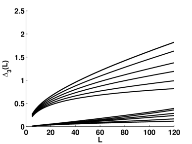
Figure 1: Here $\Delta_{3}(L,0.25,x)$ is shown for $x=0,\,2,\,4,\dots 10$, (upper lines). The calculations were for 500 spectra, with $N=400$. The standard deviation, $\sigma(400,L;x)$, corresponding to each value of $x$ (lower lines) grows rapidly with $L$. This makes the statistic much less sensitive for large $L$ values.

Now we have the tools necessary to compare a real spectrum with depleted GOE spectra in a meaningful way. After extracting $\Delta_{3}(L)$ from the data, the best value for $x$ will be the one that minimizes

$$\chi^{2}(x)=\sum^{L_{\textrm{max}}}_{L_{\textrm{min}}}\frac{[\Delta_{3}(L)-\overline{\Delta}_{3}(L,\alpha;x)]^{2}}{\sigma(N,L,\alpha;x)^{2}}.$$ (3)

Table 1: The fraction of depletion, $x$, created; the fraction determined using the $\Delta_{3}(L)$ method. The tests were run for 500 depleted spectra of size $N=90$ and 400, and with $\alpha=0.25$. The mean value, $\overline{x}$, and the standard deviation, $\sigma_{x}$ are given.

$x$	$\overline{x}\,(N=90)$	$\sigma_{x}$
3.2 %	3.2 %	3.1 %
5.3 %	4.7 %	3.4 %
8.2 %	7.3 %	2.9 %
$x$	$\overline{x}\,(N=400)$	$\sigma_{x}$
2.9 %	3.0 %	1.8%
5.0 %	5.0 %	1.9%
8.1 %	7.9 %	1.6%

For practical purposes we need an estimate of the error in $x$ from this method. To this end, we calculated the average value of $x$, and its standard deviation, for 500 GOE spectra with $N=90$ and 400 levels. The sets were made by randomly deleting 3 levels from a spectra of 93 levels, 5 out of 95, and 8 out of 98, to get spectra with $x=3.23\%$, 5.26%, and 8.16% respectively. A similar was performed for $N=400$. The results are in Table 1. Our method gave good agreement for the value of $x$, but for $N=90$ the uncertainties in $x$, $\sigma_{x}$, were of the same order as $x$, for example, with $x=5.3\%$, we get a value of $(4.7\pm 3.4)\%$. However, for $N=400$, $\sigma_{x}$ dropped to 1.9% (close to a factor of $\frac{1}{2}$) which is to be expected.

While this process for estimating the uncertainties in the fraction of missed levels is intuitive, and operationally straightforward, the results may be optimistic. There are more conservative approaches which would give larger estimates of the uncertainties. A method of calculating $\Delta_{3}(L)$ by Bohigas et al. Bohigas et al. (1984) would have us calculate $\Delta_{3}^{i}(L)$ for a much smaller number of intervals, which overlap by $L/2$. In our scheme this would translate into summing $i$ from 1 to $N-L-1$ in steps of $L/2$ in Eq. 1. An estimate of the uncertainties based on this scheme would give larger values, see Shriner Jr. and Mitchell (1992) for details.

The nearest level spacing distribution, $P(s)$, can be used to test for missing levels also. Here we will follow the work of Agvaanluvsan et al. Agvaanluvsan et al. (2003), where the maximum likelihood method is used to find the fraction of missing levels in a sequence. We tested the method on mixed, depleted, GOE spectra, and compared the results with those of our $\Delta_{3}$ analysis. $P(s)$ is known for a complete mixed GOE spectrum Guhr et al. (1998). If a level is missing, then two nearest neighbor spacings are unobserved, while one next-to-nearest spacing is included as a nearest level spacing, when it should not be. Furthermore, if $1-x$ is the fraction of the spectrum that is observed, then $D_{{\rm obs}}$, the experimental value for the average spacing, is related to the true value by $D=(1-x)D_{{\rm obs}}$. Agvaanluvsan et al. show that

$$P(s)=\sum_{k=0}^{\infty}(1-x)x^{k}P(k;s),$$ (4)

where $P(k;s)$ is the distribution function for the $k^{\textrm{th}}$ nearest neighbor spacing, $E_{k+i}-E_{i}$; for $k=0$ this reduces to $P(0;s)=P(s)$.

Given a set of level spacings $\{s_{i}\}$, the likelihood function is ${\mathcal{L}}=\prod_{i}P(s_{i})$. We are after the value of $x$ that maximizes ${\mathcal{L}}$ (although in practice it is easier to work with $\ln({\mathcal{L}})=\sum_{i}\ln P(s_{i})$). The functions $P(k;s)$ in Eq. 4 are complicated to derive, so instead of a closed form, the functions were fitted to the empirical distributions from the superposition of 1500 mixed GOE spectra, each of length $N=2000$. This was performed for each value of $\alpha$ relevant to the experimental data. Given these functions we tested the method on depleted spectra. Specifically, the procedure was tested on 1500 GOE spectra, with $N=90$ and 400, with $\alpha=0.25$; and for $N=150$, 200, 250, and 400, with $\alpha=0.4$. The depletion in each case went from 0.0% to 20% in steps of 0.5%. The error in $x$ from this method is taken to be the standard deviation of the outputted values of $x$ for the 1500 input spectra with known value of $x$. The results for $\alpha=0.25$ are shown in Table 2. The agreement with the $\Delta_{3}(L)$ method is encouraging. The $\Delta_{3}(L)$ method seems to be slightly more accurate, but the uncertainty in $x$ is slightly smaller for the MLM. Again, as with the uncertainty estimates for the $\Delta_{3}(L)$ method, the MLM uncertainties in $x$ could have been made a different way, for example Agvaanluvsan et al. Agvaanluvsan et al. (2003), use a different criterion, based on the values of the likelihood function. We have favored an approach based on distribution of results of many simulations.

Table 2: The fraction of depletion, $x$, created; the fraction determined using the maximum likelihood method. The tests were run for 1500 depleted spectra of size $N=90$ and 400, and with $\alpha=0.25$. The mean value $\overline{x}$, and the standard deviation, $\sigma_{x}$ are given.

$x$	$\overline{x}\,(N=90)$	$\sigma_{x}$
3.0 %	4.1 %	3.1 %
5.0 %	6.1 %	3.4 %
8.0 %	9.7 %	2.8 %
$x$	$\overline{x}\,(N=400)$	$\sigma_{x}$
3.0 %	3.6 %	1.6%
5.0 %	5.6 %	1.6%
8.0 %	8.7 %	1.4%

IV Nuclear data ensemble

The main idea behind using RMT to describe the fluctuations in nuclear spectra, is that each isotope corresponds to a random Hamiltonian from an ensemble with similar statistical properties as the GOE. Neutron and proton resonance data sets can be combined to make a so-called “Nuclear Data Ensemble” (NDE), see Haq et al. Haq et al. (1982). The odd-A isotopes we analyzed can be regarded as a small NDE. In Fig. 2 we have $\Delta_{3}(L)$ for each isotope (light lines), and the ensemble average (dashed line). There is a large variation in $\Delta_{3}(L)$ from spectrum to spectrum, but compare this with the situation in Fig. 3, where we see $\Delta_{3}(L)$ and $\sigma(N,L,\alpha;x)$ for 5 randomly chosen samples taken from an ensemble of GOE spectra, size $N=200$, with $\alpha=0.33$ and $x=4\%$ depletion. It is clear that variations in $\Delta_{3}(L)$ within the ensemble are normal. This is reflected in the relatively large value of $\sigma(N,L,\alpha;x)$. It is interesting to note that the plots of the level spacing distribution do not have the same variation: $P(s)$ for a particular spectrum will look like the ensemble average, see Mulhall et al. (2007).

The ensemble plot made for an NDE consisting of the data from p-wave neutrons is shown in Fig. 4. The average $\Delta_{3}(L)$ (dashed line) is consistent with an average of $x>10\%$. Compare it with the lower solid line which is $\Delta_{3}(L)$ for an ensemble of GOE spectra with $\alpha=0.33$ and $x=10\%$ depletion.

In Mulhall et al. (2007) neutron resonance data from even-even nuclei was analyzed. The ensemble plot corresponding to 9 of these isotopes is shown in Fig. 5. The isotopes represented here are ${}^{152}\text{Sm}$, ${}^{152}\text{Gd}$, ${}^{154}\text{Gd}$, ${}^{158}\text{Gd}$, ${}^{182}\text{W}$, ${}^{234}\text{U}$, ${}^{236}\text{U}$, ${}^{242}\text{Pu}$, ${}^{240}\text{Pu}$. When put into Eq. 3, the average $\Delta_{3}(L)$ for this even-even NDE gives a depletion of $x=4\%$. This is to be taken lightly, as the data comes from different facilities, over a period of decades, and is sometimes a combination of data from different experiments. It does suggest that $x=4\%$ may be typical in neutron resonance experiments, when one sequence of levels is present.

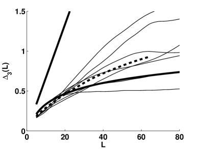
Figure 2: $\Delta_{3}(L)$ for the 7 odd-A isotopes of Tab. 3 (thin lines). The dashed line is the average of these thin lines. The lower thick line is the GOE value for $\alpha=0.4$ with no depletion ($x=0\%$). The upper thick line is for spectra with Poissonian statistics. In cases where an isotope has 2 entries in Table 3 the low energy subset is used here.

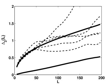
Figure 3: $\Delta_{3}(L)$, and its standard deviation vs. $L$ for 5 randomly chosen GOE spectra (dashed lines), with 4% depletion, $\alpha=0.33$, and $N=200$. The upper solid line is the ensemble average. The lower solid line is the corresponding $\sigma$.

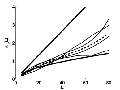
Figure 4: $\Delta_{3}(L)$ for the 4 data sets of p-wave neutrons of Tab. 4 (thin lines). The dashed line is the average of these thin lines. The lower thick line is mixed GOE spectra with $\alpha=0.4$ and 10% depletion. The upper thick line is for spectra with Poissonian statistics. In cases where an isotope has 2 entries in Table 4 the low energy subset is used here.

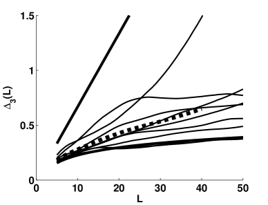
Figure 5: Here we have $\Delta_{3}(L)$ for the even-even NDE of the 9 isotopes described in Ref. Mulhall et al. (2007), the dashed line being the average value. Compare this with the pure GOE case (lower thick line). The upper thick line is the Poissonian case.

V Results and Discussion

We analyzed neutron resonance data from 11 isotopes in all. The data was taken from the Los Alamos National Laboratory website . The s-wave resonances from 7 odd-A isotopes and the p-wave resonances from 4 even-even isotopes were used. In the even-even case, the spin labels were either 1/2 or 3/2, so $\alpha=1/3$ for all 4 sets. There was a variation in the size of the sets. The ${\mathcal{N}}(E)$ plots gave us an initial idea of the completeness of the data. In Fig. 7 we see ${\mathcal{N}}(E)$ for 3 raw data sets of ${}^{58}\textmd{Cr}$, ${}^{58}\textmd{Ni}$ and ${}^{60}\textmd{Ni}$ data. The range of energy is so small compared to the neutron separation energy that one would expect ${\mathcal{N}}(E)$ to have a constant slope. A kink, where the slope (level density) gets suddenly smaller, suggests an experimental artifact that leads to missed levels. This was quite common in the data sets, which sometimes consisted of data from different facilities. In Fig. 8, for example, the see the case of ${}^{235}\textmd{U}$. There are 3 kinks in ${\mathcal{N}}(E)$, starting at $E=550$ eV. The histogram of the raw 3150 neutron resonances for ${}^{235}\textmd{U}$ is shown in Fig. 9 with the corresponding discontinuities in the level density. Notice that the kink at 550 eV in Fig. 8 corresponds to the obvious decrease in Fig. 9. Another example is in the ${}^{50}\textrm{Cr}$ data, where we see a kink at $\mathcal{N}(E)=96$ in Fig. 7. When such a kink was observed, the lower energy subset of the data (all the levels up to the kink) was examined separately. After selecting data sets the spectra were unfolded. The procedure is the same as that described in Sect. II, but ${\mathcal{N}}(E)$ was fit by a straight line, as using a higher-order polynomial would be unphysical.

The $\Delta_{3}(L)$ statistic is calculated from the data, and used to the find the value of $x$ that minimizes the quantity $\chi^{2}(x)$ in Eq. 3. The MLM was used also, and the results compared in Table 3 and 4. In what follows we compare and discuss these results, taking the odd-A isotope data first. The typical error in the value of $x$ reported from either method is 2%, based on the results in Tables 1 and 2.

V.1 ${}^{103}\textmd{Rh}$ and ${}^{147}\textmd{Sm}$

These were the only two isotopes with consistent results. Both methods suggested that only 2 or so levels were missed from the 112 ${}^{103}\textmd{Rh}$ levels, while the first 112 levels of the ${}^{147}\textmd{Sm}$ data looked complete. $\Delta_{3}(L)$ of ${}^{147}\textmd{Sm}$ lies on the $x=0\%$ line of the ensemble result, see Fig. 10. The ${\mathcal{N}}(E)$ plot for ${}^{147}\textmd{Sm}$ indicated missed levels for the remainder of the spectrum, and this was borne out by both methods, while the slope of ${\mathcal{N}}(E)$ for ${}^{103}\textmd{Rh}$ was relatively constant. See Fig. 6. The $x=6\%$ from $\Delta_{3}(L)$ is consistent with the MLM value of $x=9\%$, when reasonable error bars of 2% are used.

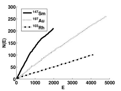
Figure 6: ${\mathcal{N}}(E)$ vs. $E$ for the ${}^{103}\textmd{Rh}$, ${}^{147}\textmd{Sm}$ and ${}^{197}\textmd{Au}$ data. Notice the change in slope after the $112^{\textrm{th}}$ level in the ${}^{147}\textmd{Sm}$ case.

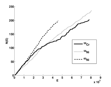
Figure 7: ${\mathcal{N}}(E)$ vs. $E$ for the raw ${}^{58}\textmd{Cr}$, ${}^{58}\textmd{Ni}$, ${}^{60}\textmd{Ni}$ data. Notice the decrease in slope after the first 100 levels in the ${}^{58}\textmd{Cr}$ data, suggesting that more levels were missed after the first 100 levels.

V.2 ${}^{167}\textmd{Er}$

The ${}^{167}\textmd{Er}$ data was missing 6% of the levels according to $\Delta_{3}(L)$, but the MLM said it was pure. Looking at a plot of ${\mathcal{N}}(E)$ will not convince you which value is preferred. There is no obvious kink, or curvature.

V.3 ${}^{185}\textmd{Re}$

The agreement regarding the ${}^{185}\textmd{Re}$ data was fine for the first 200 levels, both methods saying it was a complete set. When the full set of 477 levels was examined $\Delta_{3}(L)$ indicated over 10% of the levels were missed, while MLM still said 0%. It is unlikely that there were 0% missed in the full set, as a slope of ${\mathcal{N}}(E)$ decreases with energy.

V.4 ${}^{197}\textmd{Au}$

The first 112 levels of ${}^{197}\textmd{Au}$ look incomplete at the level of about 3% according to both methods. When the full set is analyzed, the MLM tells us that 7% are missed, but $\Delta_{3}(L)$ gives 0%. This could be a normal fluctuation, a reflection of the variation in the statistic itself, as seen in Fig. 3. An appeal to ${\mathcal{N}}(E)$ to support one result over the other is not convincing, because the graph is straight. See Fig. 6.

V.5 ${}^{241}\textmd{Pu}$

The results for ${}^{241}\textmd{Pu}$ are inconclusive. A subset was made of the first 180 levels, based on ${\mathcal{N}}(E)$. The last 57 levels had a slightly lower, but constant, density. The MLM gave $x=0\%$ in both cases, while $\Delta_{3}(L)$ gave $x=6\%$ in both cases. This disagreement is similar to that found in ${}^{167}\textmd{Er}$ case.

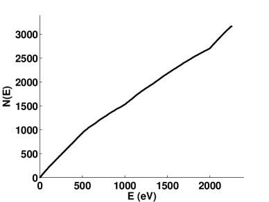
Figure 8: ${\mathcal{N}}(E)$ vs. $E$ for the raw ${}^{235}\textmd{U}$ data. Notice the decrease in slope after the first 950 levels. There are 2 other kinks, at $E=1000$ eV, and 2200 eV.

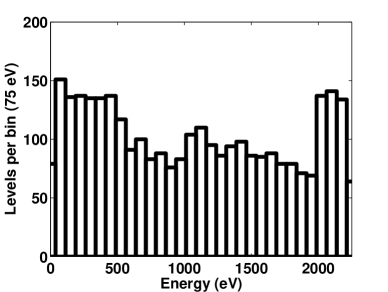
Figure 9: Histogram of the raw ${}^{235}\textmd{U}$ data. This is the slope of Fig. 8. The binsize is 75 eV. The first 950 levels span the range $0<E<500$ eV. There is a drop in the level density at 550 eV, and a sharp increase at 2000 eV, where the level density nearly doubles. This is almost certainly artificial, due to the fact that the data is the union of data from different facilities.

V.6 ${}^{235}\textmd{U}$

The ${}^{235}\textmd{U}$ is an amazing data set, because of its size and resolution. The first 950 levels were examined, as suggested by the location of the first kink in Fig. 8, at an energy of 550 eV. The abrupt change in the level density can also be seen in Fig. 9. The superposition of $j=3$ and 4 energies were analyzed together and separately. The MLM gave inconsistent results, saying the mixture of both sequences was complete, but each individual sequence was missing 2% or 3%. $\Delta_{3}(L)$ gave 1.5% missed in each separate subset. It gave 3% instead of the more consistent 1.5% for the superposition of both sequences, but these numbers agree with each other within the bounds of error. The errors in these values of $x$ are about 1%, given that $N=950$ and the errors when $N=90$ are $\approx 3\%$. This value of $x=3\%$ is very convincing when a graph of $\Delta_{3}(L)$ is examined, see Fig. 10.

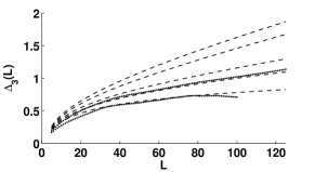
Figure 10: $\Delta_{3}(L)$ vs. $L$ for the lowest 950 levels in the ${}^{235}\textmd{U}$ (upper dots), and the lowest 112 levels of the ${}^{147}\textmd{Sm}$ (lower dots). The dashed lines are the GOE values for a mixed ($\alpha=0.4$) spectra, depleted by $x=0\%$, 3%, 5%, 8% and 10%, starting from the lowest curve. The $\Delta_{3}(L)$ analysis suggests that there are no levels missed in the ${}^{147}\textmd{Sm}$ data, and 3% of the ${}^{235}\textmd{U}$ data missed.

V.7 p-wave neutrons on even-even nuclei

The $\Delta_{3}(L)$ analysis gave $x>10\%$ for all 4 isotopes, while the MLM gave more credible results. In the case of ${}^{58}\textmd{Ni}$, the decrease in the slope of ${\mathcal{N}}(E)$ suggested that the first 116 levels looked like a more complete spectrum than the full set of 236 levels, Fig. 7. The result of the MLM analysis was consistent with this, giving $x=5.3\%$ and $7.9\%$ for these sets. The situation was the same for the ${}^{238}\textrm{U}$ data, with MLM giving $x=2.8\%$ for the first 300 levels, and $x=5.4\%$ for the full set of 1130 levels. See Table 4.

The large discrepancy in the values for $x$ is troublesome. To shed more light on this histograms of the level spacings, $s$ were compared with the GOE results for mixed spectra, with $x=0\%$ and $x=10\%$ depletion. In this case, where the possible labels for angular momentum are $1/2$ and $3/2$, we used $\alpha=1/3$. The lowest 96 ${}^{50}\textmd{Cr}$ levels, 116 ${}^{58}\textmd{Ni}$ levels, and the full set of 199 ${}^{60}\textmd{Ni}$ levels were combined into one set, see Fig. 11, and all the ${}^{238}\textmd{U}$ levels were considered as a separate set, see Fig. 12. We see in the combined set that only in the tail of $P(s)$ is the data consistent with $x\approx 10\%$, otherwise it looks undepleted. The situation for the 1130 ${}^{238}U$ levels is also perplexing in that there is an excess of small ($s<1.2$) spacings, while the tail of the histogram is consistent with $x=0$. In both cases the pictures suggest that a $\Delta_{3}(L)$ is appropriate here, and the $x>10\%$ is very unlikely indeed. Such a high fraction of missed levels would suggest that there would be a higher number of large spacings then we are seeing.

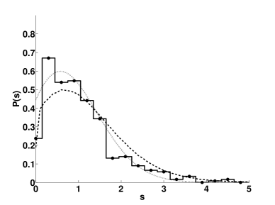
Figure 11: $P(s)$ vs. $s$ for the combined ${}^{50}\textmd{Cr}$ ${}^{58}\textmd{Ni}$ and ${}^{60}\textmd{Ni}$ data. The histogram has a bin width of 0.3, and has been normalized so that its area is unity. Also shown are the GOE results for $x=0\%$ (dotted line) and $x=10\%$ (dashed line).

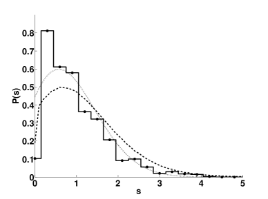
Figure 12: $P(s)$ vs. $s$ for the ${}^{238}\textmd{U}$ data. As in Fig. 11, the GOE results for $x=0\%$ (dotted line) and $x=10\%$ (dashed line) are shown.

Table 3: The results for $x$, the percent of missing levels in the data. In the last 3 rows, we separated the 950 levels from the ${}^{235}\textmd{U}$ data into the $j=3$ and $j=4$ sequences, according to the spin labels assigned in the data.

Isotope	MLM	$\Delta_{3}(L)$	$N$ (# levels)	subset
${}^{103}\textmd{Rh}$	1.6%	2%	101	All
${}^{147}\textmd{Sm}$	0.0%	0.0%	211	$1\rightarrow 112$
${}^{147}\textmd{Sm}$	9.9%	6.0%	211	All
${}^{167}\textmd{Er}$	0.0%	6.0%	113	All
${}^{185}\textmd{Re}$	0.0%	0.5%	477	$1\rightarrow 200$
${}^{185}\textmd{Re}$	0.9%	$>$10%	477	All
${}^{197}\textmd{Au}$	2.6%	4.0%	262	$1\rightarrow 119$
${}^{197}\textmd{Au}$	7.0%	0.0%	262	$120\rightarrow 262$
${}^{241}\textmd{Pu}$	0.0%	6.0%	237	$1\rightarrow 180$
${}^{241}\textmd{Pu}$	0.0%	6.0%	237	All
${}^{235}\textmd{U}\quad j=3,4$	0.0%	3.0%	3168	950
${}^{235}\textmd{U}\quad j=3$	3.4%	1.5%	1436	381
${}^{235}\textmd{U}\quad j=4$	2.1%	1.5%	1732	569

Table 4: The even-even nuclei had resonances with orbital angular momentum $L=1$, which means that these resonances had angular momentum $j=\frac{1}{2}$ or $j=\frac{3}{2}$, with mixing parameter $\alpha=\frac{1}{3}$. In these cases the $\Delta_{3}$ statistic gave $x>10\%$. The MLM was more optimistic. An uncertainty of 2% is reasonable for the MLM and $\Delta_{3}(L)$ results

Isotope	MLM	$\Delta_{3}(L)$	$N$ (# levels)	subset
${}^{50}\textmd{Cr}$	3.9%	$>$10%	203	$1\rightarrow 96$
${}^{58}\textmd{Ni}$	5.3%	$>$10%	236	$1\rightarrow 116$
${}^{58}\textmd{Ni}$	7.9%	$>$10%	236	All
${}^{60}\textmd{Ni}$	11.6%	$>$10%	199	All
${}^{238}\textmd{U}$	2.8%	$>$10%	1130	$1\rightarrow 300$
${}^{238}\textmd{U}$	5.4%	$>$10%	1130	All

VI Conclusion

The $\Delta_{3}(L)$ statistic was used to determine the completeness of neutron resonance data for 7 different odd-$A$ isotopes, and p-wave neutrons on 4 even-even isotopes. These are difficult data to work with due to the presence of 2 independent sequences of levels that do not repel each other. This means there is a much higher incidence of small level spacing, making it much more difficult to get a complete set of data. A method of estimating the fraction, $x$ of missed levels, based on $\Delta_{3}(L)$ was presented. The method was tested on numerical realizations of depleted and mixed GOEs. Experimental data was grouped into Nuclear Data Ensembles, and $\Delta_{3}(L)$ calculated. The behavior was consistent with the overarching theme of RMT. Results were compared with the maximum likelihood method. There were 13 data sets made from the 7 odd-A isotopes (including subsets for the same isotope). The MLM was in agreement with the $\Delta_{3}(L)$ method in 7 out of these 13 data sets. Of the 6 sets where there was discordance, it looked like there was only one case where the MLM result made more intuitive sense, (${}^{197}\textmd{Au}$, levels 120 to 262). In the other 5, it is difficult to say which method, if any, is more likely to be correct. In the 6 data sets made from the 4 even-even isotopes, the MLM gave a variety of consistent results, while $\Delta_{3}(L)$ gave $x>10\%$ for all sets. A plot of $P(s)$ and a comparison with the GOE results suggest that a $\Delta_{3}(L)$ analysis is not appropriate here. The cumulative level number ${\mathcal{N}}(E)$ was used as another indicator of the purity of the data, and the credibility of the results from the two statistics. A strong case has been made for the usefulness of the $\Delta_{3}(L)$ statistic as a gauge of the completeness of a data set when a RMT analysis is appropriate.