Rigorous results for tight-binding networks: particle trapping and scattering

Abstract

We investigate the particle trapping and scattering properties in a tight-binding network which consists of several subgraphs. The particle trapping condition is proved under which particles can be trapped in a subgraph without leaking. Based on exact solutions for the configuration of a $\pi$-shaped lattice, it is argued that the bound states in a specified subgraph are of two types, resonant and evanescent. We also link the trapping rigorous result to the scattering problem. The scattering features of the $\pi$-shaped lattice is investigated in the framework of the Bethe Ansatz.

I Introduction

Trapping and scattering of a particle is an important feature in many quantum information processing systems. Due to the development of technology, the implementation of quantum information processing in quantum systems with periodic potential, such as optical lattices OL , arrays of quantum dots QD , photonic crystal PC and coupled-resonator optical waveguide CROW , has attracted intensive investigations. The design of quantum device based on these promising technologies relies on the particle trapping and scattering properties in a discrete system. A heuristic example shows that the quantum confinement in a discrete system is distinct from its counterpart in continuum media Longhi PRE , due to the Wannier-Stark localization Fukuyama .

This paper focuses on noninteracting particles on discrete lattice, which is treated by tight-binding approximation. Intuitively, the particle trapping is implemented by sufficient strong on-site potential as the continuous system. In contrast to continuum, however, different dynamical properties emerge in the lattice system due to its distinct dispersion relation: a local wave packet can be confined by linear potential distribution Longhi PRE and the degree of spreading of a propagating wave packet can be controlled by judicious choice of the particle energy Osborne ; Yang PRA ; Kim PRB . Recent studies show that Fano resonance may be employed to construct the perfect mirror or transparency so as to control particles in a region of the lattice ZhouL1 ; ZhouL2 ; Liao via engineered configurations. Because of the numerous varieties of the possible geometry of the quantum network, we believe it is beneficial to have lattice-based rigorous results and exact solutions for the devise of a quantum device. In this paper, we show rigorously that the perfect particle trapping without any leakage can be achieved in simple tight-binding networks. This provides a method to devise the quantum network to confine particles with required mode. We also link the trapping rigorous result to the scattering problem. This general finding is illustrated by a practical network consisting of a waveguide with an embedded $\pi$-shaped subgraph. Exact solutions for such types of configurations are obtained to demonstrate and supplement the rigorous results.

II Rigorous result for particle trapping

A general tight-binding network is constructed topologically by the sites and the various connections between them, and is also represented as a vertex-edge graph. Cutting off some of the connections, a graph is decomposed into several subgraphs. So when a particle is strictly trapped within a certain region of a network, one can say that it is confined in a specified subgraph. The main aim of this paper is to answer the questions of what kind of subgraph can trap a particle as bound state and of how such a subgraph scatters a particle when it is embedded in a waveguide.

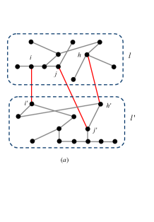
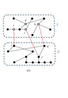
Figure 1: (Color online) An arbitrary graph of tight-binding network within part of which particles may be confined without any leakage. The graph can be decomposed into two subgraphs $l$ and $l^{\prime}$ which are connected via the coupling between the joint sites $(i,j,h)$ and $(i^{\prime},j^{\prime},h^{\prime})$ (a). The perfect bound states can be formed in subgraph $l$ when the eigen functions of $H_{l}$ have wave nodes on all the joint sites $(i,j,h)$, which are denoted by empty circles (b). The existence of more wave nodes (like site $g$) may allow multiple bound states.

The Hamiltonian of a tight-binding network, or a graph which consists of $n_{0}$ subgraphs reads as

$$H = \sum_{l=1}^{n_{0}}H_{l}+\sum_{lm}H_{lm},$$ (1)

$$H_{l} = -\sum_{\left\langle ij\right\rangle}(\kappa_{ij}^{[l]}a_{l,i}^{{\dagger}}a_{l,j}+\text{H.c.})+\sum_{i=1}^{N_{l}}\mu_{i}^{[l]}a_{l,i}^{{\dagger}}a_{l,i},$$

$$H_{lm} = -\sum_{i,j}(\kappa_{ij}^{[lm]}a_{l,i}^{{\dagger}}a_{m,j}+\text{H.c.}),$$

where label $l$ denotes the $l$th subgraph of $N_{l}$ site, which subgraph is defined by the distribution of the hopping integrals $\{\kappa_{ij}^{[l]}\}$ and on-site potentials $\{\mu_{i}^{[l]}\}$, and $a_{l,j}^{{\dagger}}$ is the boson or fermion creation operator at the $j$th site in the $l$th subgraph. Here, $H_{l}$ and $H_{lm}$ represent the Hamiltonians of the subgraphs and the couplings between them. In terms $H_{lm}$, site $i$ $(j)$ is the joint site of subgraph $l$ $(m)$ for the connections to other subgraphs. Obviously, the decomposition of subgraphs is arbitrary, and can be implemented at will. Figure 1 shows an example schematically. Note that the Hamiltonians $H_{l}$ (also $H$) are quadratic in particle operators and can be diagonalized through the linear transformation

$$\eta_{l,k}^{{\dagger}}=\sum_{j}g_{k,j}^{l}a_{l,j}^{{\dagger}}$$ (2)

which leads to

$$H_{l}=\sum_{k}\varepsilon_{l,k}\eta_{l,k}^{{\dagger}}\eta_{l,k},$$ (3)

where $\varepsilon_{l,k}$ is the corresponding eigenvalue of $H_{l}$ for the eigenfunction $g_{k,j}^{l}$. Site $j$ is defined as the wave node for the eigen mode $k$ of graph $l$ if we have $g_{k,j}^{l}=0$. We denote the wave node as $j(l,k)$, which reflects the property of the eigen state $\eta_{l,k}^{{\dagger}}\left|0\right\rangle$ of $H_{l}$

$$a_{l,j}\eta_{l,k}^{{\dagger}}\left|0\right\rangle=0,$$ (4)

where $\left|0\right\rangle$ is the vacuum state. Now we consider the case of that all the joint sites of the subgraph $l$ are the wave nodes of eigen mode $k$. Under this condition, we have

$$H\left(\eta_{l,k}^{{\dagger}}\left|0\right\rangle\right)=H_{l}\left(\eta_{l,k}^{{\dagger}}\left|0\right\rangle\right)=\varepsilon_{l,k}\left(\eta_{l,k}^{{\dagger}}\left|0\right\rangle\right),$$ (5)

i.e., the eigen state $\eta_{l,k}^{{\dagger}}\left|0\right\rangle$ is also the eigen state of the whole graph $H$. Then such a state represents the trapping or bound state of a particle within the subgraph $l$ with infinite life time. This rigorous conclusion has important implications in the design of quantum network to store particles in the target region at will. Figure 1 represents an arbitrary graph of tight-binding network within part of which particles can be confined without any leakage. The whole graph can be decomposed into two subgraphs $l$ and $l^{\prime}$ which are connected via the couplings between the joint sites $(i,j,h)$ and $(i^{\prime},j^{\prime},h^{\prime})$. The perfect bound state can be formed in subgraph $l$ as the eigen function of $H_{l}$ when it has wave nodes on all the joint sites $(i,j,h)$. The existence of additional wave nodes indicates the multiple bound states can be formed.

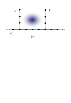
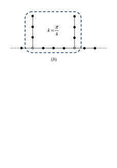
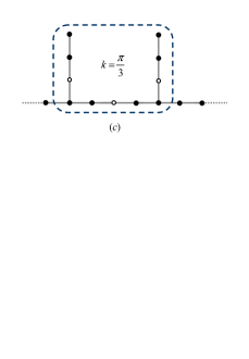
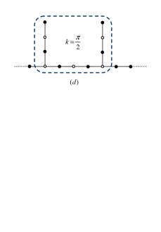
Figure 2: (Color online) Configuration of $\pi$-shaped lattice that admits the formation of trapping particles. It consists of three chains $A$, $B$ and $C$. Two three-site chains $A$ and $B$ are side coupled to the chain $C$ with arbitrary number of sites (a). This graph can be decomposed into three subgraphs, one of which is eleven-site chain enclosed by the dashed rectangular. The single-particle eigen states of the eleven-site chain with quasi momenta $k=\pi/4,\pi/3,$ and $\pi/2$ have two, three and four wave nodes, denoted by empty circles in (b), (c) and (d). For states with $k=\pi/4$ and $\pi/2$, the joint sites being all wave nodes, the particle can be trapped in the eleven-site chain, while state with $k=\pi/3$ is not a bound state. States with other values of $k$ can be analyzed accordingly.

III Demonstration configurations

Now we investigate a class of practical examples to demonstrate the application of the result above. We consider a system of $\pi$-shaped lattice (Figure 2), consisting of an infinite chain side coupling to two finite chains of length $N_{0}$ at the joint sites $1$ and $L$, which has the Hamiltonian

$$H = H_{a}+H_{b}+H_{c}+H_{\text{joint}},$$ (6)

$$H_{a}+H_{b} = -\kappa_{0}\sum_{i=1}^{N_{0}}(a_{i}^{{\dagger}}a_{i+1}+b_{i}^{{\dagger}}b_{i+1}+\text{H.c.}),$$

$$H_{c} = -\kappa\sum_{i=-\infty}^{\infty}(c_{i}^{{\dagger}}c_{i+1}+\text{H.c.}),$$

$$H_{\text{joint}} = -\kappa_{0}(a_{1}^{{\dagger}}c_{1}+b_{1}^{{\dagger}}c_{L}+\text{H.c.}),$$

where $a_{j}^{{\dagger}}$ ($b_{j}^{{\dagger}}$ and $c_{j}^{{\dagger}}$) is the boson or fermion creation operator at the $j$th site in the chain $a$ ($b$ and $c$). The side coupling model was employed to depict coupled-cavity system for stopping and storing light coherently Fan . For the simple case with the shortest side chains, i.e. $N_{0}=1$, the configuration is equivalent to the atom-cavity system with single excitation ZhouL1 ; ZhouL2 , where the side-site state represents the excited state of the two-level atom.

First of all, we consider a simplest case: the hopping integrals are identical for all chains, i.e., $\kappa=\kappa_{0}$. This graph can be decomposed into three subgraphs: left chain, right chain and central chain of $\Lambda=2N_{0}+L$ sites. The eigen wave functions of the central chain are given by

$$g_{k,j}=\sqrt{\frac{2}{\Lambda+1}}\sin kj,\text{ }j\in[1,\Lambda],$$ (7)

where $k=n\pi/\left(\Lambda+1\right)$, $n\in[1,\Lambda]$, with corresponding eigen values $-2\kappa\cos k$. These states possess the wave nodes at

$$j_{k}=\frac{\left(\Lambda+1\right)m}{n},$$ (8)

where $m$ are certain integers which ensure the existence of integer $j_{k}$ for a given $n$. Then in the case of that $\left\{j_{k}\right\}$ cover the joint sites $N_{0}+1$ and $N_{0}+L$ simultaneously, the corresponding eigen states are the trapping states, i.e., a particle can be hold along the central chain forever. An example of $N_{0}=3$, $L=5$ is depicted in Figure 2, where only typical cases with $k=\pi/4,\pi/3,$ and $\pi/2$ are presented. Actually, [Eq. (8)] shows that states with $k=\pi/4,$ $\pi/2,$ and $3\pi/4$ have wave nodes at the joint sites. Therefore there are three resonant bound states for this configuration. It has been proposed that such kind of trapping state can act as a cavity when a boson system is considered ZhouL2 . Remarkably, two peculiar features are identified. First, the bound state has infinite life time in the ideal case without decoherence since it is based on the mechanism of Fano interference rather than two potential barriers. Second, the number of the cavity mode does not solely depend on the size of the cavity $L$ like the case of using infinite potential well for particle trapping. For example, taking $N_{0}=1$, one can achieve a single mode cavity with $k=\pi/2$ for arbitrary odd $L$, but none for even $L$. Meanwhile, it will be shown later that there is another type of bound state, evanescent bound state. Besides these exact bound states, there exist eigen states of the subgraph which have nonzero, but very small probability at the joint sites in the case of large $L$. Such kind of state has finite but long life times, which is called quasi resonant bound states. To demonstrate these concepts, we present a numerical simulation of the damping process for various modes in two typical systems with $N_{0}=2$, $L=4$ and $N_{0}=3$, $L=123$, respectively. A particle is initially located in the subgraph in the eigen states $\left|k\right\rangle$ [Eq. (7)]. We investigate the dynamics of the states by computing the quantity

$$P(k,t)=\left\langle\sum_{i=1}^{N_{0}}(a_{i}^{{\dagger}}a_{i}+b_{i}^{{\dagger}}b_{i})+\sum_{i=1}^{L}c_{i}^{{\dagger}}c_{i}\right\rangle_{k,t},$$ (9)

where $\left\langle...\right\rangle_{k,t}$ denotes the expectation value of the probability of the particle within the subgraph for an evolved state $\exp\left(-iHt\right)\left|k\right\rangle$. Figure 3 shows the numerical simulation of $P(k,t)$ as functions of the mode $k$ and time $t$ for a short $L$ in the upper plot while for a longer $L$ in the lower plot. There are three types of curves in the two plots: (i) remaining unitary; (ii) damping slowly; (iii) dropping drastically and then keeping at a finite value. Cases (i) occurs in both two configurations, corresponding to perfect resonant bound states. Case (ii) occurs in large-$L$ system, corresponding to quasi resonant bound state (we omit such kind of curve in the lower panel). Case (iii) occurs in small-$L$ system, corresponding to another type of bound state, evanescent bound state, which will be discussed in detail later.

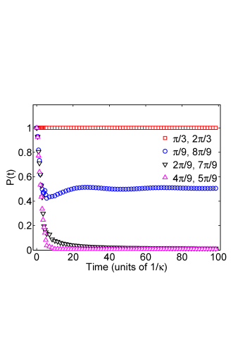
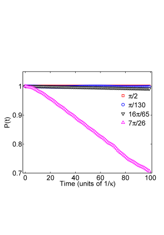
Figure 3: (Color online) The probability $P(k,t)$ of a particle, initially located in the state $\left|k\right\rangle$,  remaining in the subgraph. The simulations are performed in two typical systems with $N_{0}=2$, $L=4$ (upper panel) and $N_{0}=3$, $L=123$ (lower panel), respectively. The shapes of all the curves can be classified into three types as mentioned in the text.

A resonant bound-state configuration can be understood from the point of view of interference. The bound state we constructed in this manner is the standing-wave like state in the subgraph. In general, the formation of a standing wave in a quantum system is due to the infinite potential barriers which reflect the wave with any momentum. Then there is no additional condition for the distance between two barriers. In a tight-binding network, a side coupled chain can act as the infinite potential barriers for the incident wave with certain momentum. As an example, it can be readily shown by the method below that, for an incident wave with $k=\pi/2$, the transmission coefficient $T$ through one side coupled chain of length $N_{0}$ can be expressed as $T=\left[1+(-1)^{N_{0}}\right]/2$. It has been discussed in Ref. ZhouL1 ; ZhouL2 for the case of $N_{0}=1$. Besides the mirror condition $T=0$, a matching distance between two side coupled chains is also required to form a standing wave. This will be discussed below in the aid of exact results.

In the above analysis, the trapping subgraph is the simplest lattice, an open chain. There are some a little more complicated subgraphs, the hierarchical lattices, as the demonstration configurations. It has been shown that ZLin ; Cha96 ; Cha01 there are eigen wave functions of these hierarchical lattices, whose amplitudes are zero at certain sites. When these lattices are embedded in a network by linking the nodes only, the trapping states are formed. Considering an arbitrary generation Vicsek fractal as an example, there is eigen wave function whose amplitude is zero at the center of every five-site cell. Then when such a lattice is embedded in a network by linking the center sites only, the corresponding eigenstate is the trapping state with respect to the network. Nevertheless, for the hierarchical lattice itself, this eigenstate becomes an extended state as its size grows up.

IV Bethe Ansatz results

We now turn to discuss the complete bound states in a subgraph by taking the network of [Eq. (6)] as an example. It is worthy to point out that the bound states constructed by the before-mentioned method are not complete. In the following it will be shown that there are two types of bound states: resonant and evanescent. The former describes trapped particle in a specified spatial region and the later describes particle with an exponentially decaying probability beyond a specified spatial region. In the following, we investigate this problem based on the Bethe Ansatz approach. Actually, the bound-state wave functions $\psi(j)$ of the Hamiltonian [Eq. (6)] can be expressed as a piecewise function over all sites

$$\psi_{c}(j) = \left\{\begin{array}[]{ll}C_{1}e^{-ik\left(j-1\right)}&\text{ \ \ for }j\leq 1,\\ C_{2}e^{ikj}+C_{3}e^{-ikj}&\text{ \ \ for }2\prec j\prec L,\\ C_{4}e^{ik\left(j-L\right)}&\text{ \ \ for }j\geq L,\end{array}\right.$$

$$\psi_{a}(j) = A_{1}e^{iqj}+A_{2}e^{-iqj}\text{ \ \ for }1\leq j\leq N_{0},$$

$$\psi_{b}(j) = B_{1}e^{iqj}+B_{2}e^{-iqj}\text{ \ \ for }1\leq j\leq N_{0}.$$

Here $\psi_{a,b,c}$ denote wave functions along chains $a$, $b$, and $c$, respectively. The coefficients and momenta $C_{1,2,3,4}$, $A_{1,2}$, $B_{1,2}$, $k$, and $q$ are determined by matching conditions and the corresponding Schrodinger equations Hirsch

$$\psi\left(j+0^{+}\right)=\psi\left(j+0^{-}\right),$$ (11)

$$-\kappa_{j+1,j}\psi\left(j+1\right)-\kappa_{j-1,j}\psi\left(j-1\right) =E\psi\left(j\right).$$ (12)

where $E$ is eigen energy, $\kappa_{j\pm 1,j}$ are the corresponding hopping integrals. The solutions can be classified in two categories: resonant and evanescent ones, which correspond to zero and nonzero $C_{1,4}$, respectively.

For the resonant bound states, zero $C_{1,4}$ lead to zero particle probability at the joint points, which is consistent with the above mentioned rigorous results. In addition, the momenta $k$ and $q$ are determined by equations

$$\sin\left[k\left(L-1\right)\right] = \sin\left[q\left(N_{0}+1\right)\right]=0,$$ (13)

$$E = -2\kappa_{0}\cos q=-2\kappa\cos k.$$ (14)

For simplicity, only simple cases with $\kappa_{0}=\kappa$ are considered to demonstrate and explore the obtained rigorous results. The existence of the solution requires $\left(L-1\right)m=\left(N_{0}+1\right)n$, where $n\in[1,L-2]$ and $m\in[1,N_{0}]$. Obviously, the resonant bound states in the above mentioned example with $N_{0}=3$ and $L=5$ is the simplest case of $m=n=1$, $2$, and $3$, corresponding to momenta $\pi/4$, $\pi/2$, and $3\pi/4$, respectively.

For the evanescent bound state, which possesses nonzero particle probability at and around the joint points, the momenta $k$ and $q$ are determined by equations

$$\frac{\kappa\zeta\left(k\right)}{\zeta\left(k\left(L-1\right)\right)}\left[e^{-ik\left(L-1\right)}\pm 1\right] = \frac{\kappa_{0}\zeta\left(qN_{0}\right)}{\zeta\left(q\left(N_{0}+1\right)\right)},$$ (15)

$$E=-2\kappa_{0}\eta\left(q\right)=-2\kappa\eta\left(k\right),$$ (16)

where $\zeta\left(\theta\right)=$ $\left(e^{i\theta}-e^{-i\theta}\right)/2$ and $\eta\left(\theta\right)=$ $\left(e^{i\theta}+e^{-i\theta}\right)/2$. Taking $\kappa_{0}=\kappa$, $N_{0}=3$, and $L=5$ as an example, we have $q=k=0.382i$, $\pi+0.382i$, or $0.191i$, $\pi+0.191i$, which correspond to symmetric and antisymmetric evanescent bound eigen functions, respectively. Furthermore, for the case of $\kappa_{0}=\kappa$, $N_{0}=2$, and $L=4$, plotted in Figure 3, we have $q=k=0.382i$ or $\pi+0.382i$. Accordingly, three initial states with momenta $\pi/9$, $2\pi/9$, and $4\pi/9$, as well as their counterparts have nonzero overlaps with the two evanescent bound states. We are then able to obtain the long-time behavior of $P(t)$ as $0.5032$, $0.0027$, and $0.0058$, which are in agreement with the plots in the upper panel of Figure 3.

V Scattering problems

In general, trapping and scattering are two contrary phenomena which always refer to localized and extended states. In the context of this paper, the resonant bound state is essentially standing wave like, consisting of two constituents: incident and reflected waves. On the other hand, the rigorous result for such bound states has no restriction to the size and geometry of the subgraph and is applicable to the scattering problem. This is another main issue we want to stress in this paper.

For scattering problem, the input, output waveguides and the center system should be involved. One can take the input waveguide, which is usually semi-infinite chain, together with a part of the center system as the subgraph. The resonant bound state in such a subgraph corresponds to a total reflection. Actually, the trapping wave function within the input waveguide region is the superposition of two opposite travelling plane waves with the identical amplitudes. They correspond to the incident and total reflected waves. And the eigen energy $E$ of this trapping state is exactly the transmission zero, i.e., $T(E)=0$. Taking the above $\pi$-shaped lattice as an illustrated example, the subgraph containing the input waveguide is depicted by the Hamiltonian

$$H_{in}=-\kappa\left(\sum_{i=1}^{N_{0}}a_{i}^{{\dagger}}a_{i+1}+a_{1}^{{\dagger}}c_{1}+\sum_{i=-\infty}^{1}c_{i}^{{\dagger}}c_{i+1}+\text{H.c.}\right),$$ (17)

which is a uniform semi-infinite chain. The resonant bound states must have a node at site $c_{1}$ with energy $E=-2\kappa\cos q$, where $q$ is determined by the position of the node, $\sin\left[q\left(N_{0}+1\right)\right]=0$.

Now we consider the scattering problem of the $\pi$-shaped lattice, demonstrating the relation linking the scattering state and resonant bound state in the framework of the Bethe Ansatz. It is worth to note that many efforts have been devoted to discuss critically the effect of a dangling side coupled chain on the spectrum and transmission properties of a linear chain, including the Fano resonance, by approximate approaches AY ; PF ; Cha06 ; Cha07 .

In a $\pi$-shaped lattice, the scattering wave function has the form

$$\psi_{c}(j) = \left\{\begin{array}[]{ll}e^{ik\left(j-1\right)}+re^{-ik\left(j-1\right)}&\text{ \ \ for }j\leq 1,\\ Ae^{ik\left(j-1\right)}+Be^{-ik\left(j-1\right)}&\text{ \ \ for }2\prec j\prec L,\\ te^{ik\left(j-1\right)}&\text{ \ \ for }j\geq L,\end{array}\right.$$

$$\psi_{a}(j) = C_{a}e^{iqj}+D_{a}e^{-iqj},\text{ \ \ for }1\leq j\leq N_{0},$$

$$\psi_{b}(j) = C_{b}e^{iqj}+D_{b}e^{-iqj},\text{ \ \ for }1\leq j\leq N_{0}.$$

where $r$ and $t$ are reflection and transmission amplitudes for an incident wave with momentum $k$. Similarly, applying the matching conditions [Eq. (11)] and the corresponding Schrodinger equations [Eq. (12)], we then obtain

$$t=\frac{\alpha^{2}\sin^{2}k}{\alpha^{2}\sin^{2}k-i\alpha\beta\sin k+\left(\beta/2\right)^{2}\left[e^{i2k\left(L-1\right)}-1\right]}$$ (19)

where $\alpha=\kappa\sin\left[q\left(N_{0}+1\right)\right]$ and $\beta=\kappa_{0}\sin\left(qN_{0}\right)$. Note that zero $\alpha$ leads to vanishing of $t$, while zero $\beta$ leads to vanishing of $r$. The former and latter are in agreement with the conclusions of the above analysis from the interference point of view for the total reflection and resonant transmission, respectively.

From Eq. (19), the transmission probability has the form

$$T=\frac{\alpha^{4}\sin^{4}k}{\alpha^{4}\sin^{4}k+\left(\beta/2\right)^{2}\left(\beta^{2}+4\alpha^{2}\sin^{2}k\right)\sin^{2}\left[k\left(L-1\right)-\delta\right]}$$ (20)

where $\tan\delta=2\alpha\sin k/\beta$. Eq. (20) allows the analytical investigation on the transmission features. First, it is found that the total reflection condition coincides with the resonant bound condition Eq. (13). It indicates the conclusion that an incident wave is totally reflected by the side coupled chains if its energy exactly equals to the resonant bound state energy. The same conclusion has been obtained for some similar systems AY ; PF ; Cha06 ; Cha07 . This is a direct result from the fact that the scattering of any dangling side coupled chain is isotropic for the incident waves from both sides along the waveguide. On the other hand, the resonant transmission condition is also easy to be understood from the aspect of wave nodes in the subgraph. In fact equation $\sin\left(qN_{0}\right)=0$ indicates the effective disconnection of the wave guide from the side coupled system.

Second, for a fixed $N_{0}$, the common transmission zeros and reflection zeros for arbitrary $L$ can be simply determined by $\alpha=0$ and $\beta=0$, respectively. More precisely, for the incident waves with $k_{\min}=\cos^{-1}\left\{\left(\kappa_{0}/\kappa\right)\cos\left[n\pi/\left(N_{0}+1\right)\right]\right\}$, $n\in Z$, we have $T=0$, while the one with $k_{\max}=\cos^{-1}\left[\left(\kappa_{0}/\kappa\right)\cos\left(n\pi/N_{0}\right)\right]$, we have $T=1$. The rest reflection zeros are $L$-dependent and determined by $\sin^{2}\left[k\left(L-1\right)-\delta\right]=0$.

The transmission spectra are plotted for $\kappa=\kappa_{0}$, $N_{0}=2$ ,$3$ and different $L$ in Fig. 4 as illustration. We can see that the common transmission zeros occur at $E=-1$ for $N_{0}=2$; $E=-\sqrt{2}$ for $N_{0}=3$, while the common reflection zeros occur at $E=0$ for $N_{0}=2;$ $E=-1$ for $N_{0}=3$, which are in agreement with the above analysis. From the plots, one can find that it does not exhibit perfect Fano line shape. Nevertheless, the peak and dips profiles are the direct result of interference result from subwaves in different paths. Actually, the formations of $k_{\min}$ and $k_{\max}$ correspond to the complete destructive and constructive interferences.

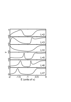
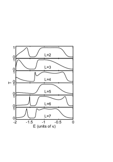
Figure 4: The plots of $T(E)$ from Eq. (20) for the systems of $N_{0}=2$ (left), $3$ (right) with different $L$.

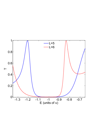
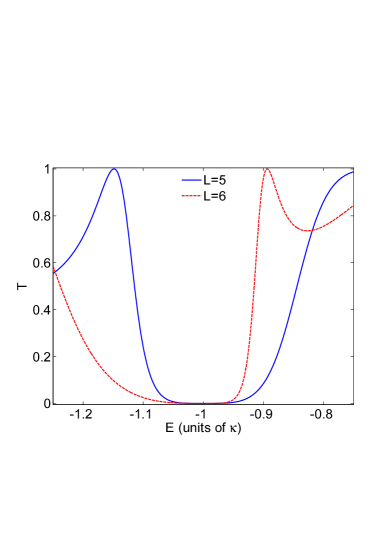
Figure 5: (Color online) Transmission probability $T(E)$ for the configurations with $N_{0}=2$ (up panel), $5$ (down panel) and $L=5$ (solid blue line), $L=6$ (dashed red line). The plots show the evident swapping of peak-dip profiles.

Now we focus on the $L$-dependent reflection zeros. Consider a system with fixed $L=L_{0}$, the $L$-dependent reflection zeros occur at $k_{0}$, which satisfies

$$\sin^{2}\left[k_{0}\left(L_{0}-1\right)-\delta\right]=0.$$ (21)

Meanwhile, for a system with $L=L_{0}+m$, the corresponding transmission coefficient obeys

$$T\left(k_{0},L_{0}+m\right)=T\left(k_{0},L_{0}-m\right)$$ (22)

for $L_{0}-m\succ 0$, due to the identity

$$\sin^{2}\left[k_{0}\left(L_{0}+m-1\right)-\delta\right]=\sin^{2}\left(mk_{0}\right).$$ (23)

This fact leads to an interesting conclusion. For a certain $k_{0}$, if there are two systems $L$ and $L^{\prime}$ that satisfy $T\left(k_{0},L\right)=$ $T\left(k_{0},L^{\prime}\right)=1$, there should exist a series of different $L,L^{\prime},L^{\prime\prime},L^{\prime\prime\prime},...,$ satisfy $T\left(k_{0},L^{\prime\prime}\right)=$ $T\left(k_{0},L^{\prime\prime\prime}\right)=...=1$. Especially, applying this conclusion for $m=1$ case, it follows that there is no $k_{0}$ to satisfy $T\left(k_{0},L\right)=$ $T\left(k_{0},L+1\right)=1$, except the common reflection zeros. In other words, there is no $L$-dependent reflection zeros for $L$ and $L+1$ meeting at the same $k$. This feature enhance the probability of the occurrence of so called peak-dip swapping as $L$ changes Cha06 ; Cha07 .

For a fixed $N_{0}$, one can always find two systems with successive $L$, that they have at least one peak (reflection zero) located at each side of a common dip (transmission zero). Since there is only one peak at each $k_{0}$, the peak-dip swapping profile is formed in the vicinity of a common dip. Here we exemplify this point by investigating the cases with $\kappa=\kappa_{0}$ and small $N_{0}$. For $N_{0}=2$, one of the common transmission zero is $k_{\min}=\pi/3$, while the $L$-dependent reflection zeros are determined by $\sin^{2}\left[k_{0}\left(L_{0}-1\right)-\delta\right]$ $=0$. The closest (or closer) solution of $k_{0}$ around $k_{\min}=\pi/3$ are the left one $k_{0L}=0.29\pi$ ($E=-1.21$) for $L=5$, and the right one $k_{0R}=0.36\pi$ ($E=-0.84$) for $L=6$. The profiles of the corresponding transmission spectra are plotted in Fig. 5 (upper), which exhibit the same character as the one in Fig. 7 of Ref. Cha06 . Another example for $N_{0}=5$ and $L=5$, $6$, is also plotted in Fig. 5 (lower). One can see the occurrence of the profile of evident peak-dip swapping.

VI Summary

In summary, we show in this paper, within the context of a tight-binding model, that a particle can be trapped in a nontrivial subgraph. As an application, we examine concrete networks consisting of a $\pi$-shaped lattice. Exact solutions for such types of configurations are obtained to demonstrate and supplement the rigorous results. It is shown that there are two types of bound states: resonant and evanescent. We also link the trapping rigorous result to the scattering problem for such a subgraph being embedded in a one-dimensional chain as the waveguide. It is shown that an incident wave experiences total reflection under certain condition. Finally, we also investigate the scattering features of the $\pi$-shaped lattice in the framework of the Bethe Ansatz. Such rigorous results are expected to be necessary and insightful for quantum control and engineering.

We acknowledge the support of the CNSF (Grants No. 10874091 and No. 2006CB921205).

References

- (1) O. Mandel, M. Greiner, A. Widera, T. Rom, T. W. Hänsch, and I. Bloch, Nature (London) 425, 937 (2003).
- (2) B. E. Kane, Nature (London) 393, 133 (1998); D. Loss and D. P. DiVincenzo, Phys. Rev. A 57, 120 (1998).
- (3) J. Bravo-Abad and M. Soljačić, Nature Mater. 6, 799 (2007); Y. Tanaka, J. Upham, T. Nagashima, T. Sugiya, T. Asano, and S. Noda, Nature Mater. 6, 862 (2007).
- (4) M. Sandberg, C. M. Wilson, F. Persson, T. Bauch, G. Johansson, V. Shumeiko, T. Duty, and P. Delsing, Appl. Phys. Lett. 92, 203501 (2008); M. A. Castellanos-Beltran and K. W. Lehnert, Appl. Phys. Lett. 91, 083509 (2007).
- (5) S. Longhi, Phys. Rev. E 75, 026606 (2007).
- (6) H. Fukuyama, R.A. Bari, and H.C. Fogedby, Phys. Rev. B 8, 5579 (1973).
- (7) T. J. Osborne and N. Linden, Phys. Rev. A 69, 052315 (2004).
- (8) S. Yang, Z. Song and C. P. Sun, Phys. Rev. A 73, 022317 (2006).
- (9) W. Kim, L. Covaci, and F. Marsiglio, Phys. Rev. B 74, 205120 (2006).
- (10) L. Zhou, Z. R. Gong, Y. X. Liu, C. P. Sun, and F. Nori, Phys. Rev. Lett. 101, 100501 (2008).
- (11) L. Zhou, H. Dong, Y. X. Liu, C. P. Sun, and F. Nori, Phys. Rev. A 78, 063827 (2008).
- (12) J. Q. Liao, J. F. Huang, Y. X. Liu, L. M. Kuang, and C. P. Sun, e-print arXiv:0904.0844v1.
- (13) M. F. Yanik and S. H. Fan, Phys. Rev. Lett. 92, 083901 (2004); M. F. Yanik and S. H. Fan Phys. Rev. A 71, 013803 (2005).
- (14) Z. Lin and M. Goda, J. Phys. A: Math. Gen. 26, L1217 (1993).
- (15) A. Chakrabarti and B. Bhattacharyya, Phys. Rev. B 54, R12625 (1996).
- (16) A. Chakraborti, B. Bhattacharyya and A. Chakrabarti, Phys. Rev. B 61, 7395 (2000).
- (17) J. E. Hirsch, Phys. Rev. B 50, 3165 (1994).
- (18) A. E. Miroshnichenko and Y. S. Kivshar, Phys. Rev. E 72, 056611 (2005).
- (19) P. A. Orellana, F. Domínguez-Adame, I. Gómez, and M. L. Ladrón de Guevara, Phys. Rev. B 67, 085321 (2003).
- (20) A. Chakrabarti, Phys. Rev. B 74, 205315 (2006).
- (21) A. Chakrabarti, Phys. Lett. A 366, 507 (2007).