Abstract

We construct a warm inflation model with inflaton field non-minimally coupled to induced gravity on a warped DGP brane. We incorporate possible modification of the induced gravity on the brane in the spirit of $f(R)$-gravity. We study cosmological perturbations in this setup. In the case of two field inflation such as warm inflation, usually entropy perturbations are generated. While it is expected that in the case of one field inflation these perturbations to be removed, we show that even in the absence of the radiation field, entropy perturbations are generated in our setup due to non-minimal coupling and modification of the induced gravity. We study the effect of dissipation on the inflation parameters of this extended braneworld scenario.
PACS: 04.50.-h,  98.80.-k,  98.80.cq,  98.80.Es
Key Words: Braneworld Gravity, Scalar-Tensor Theories, Induced Gravity, Warm Inflation, Perturbations

1 Introduction

The idea of inflation is a very successful paradigm to solve the problems of the standard cosmology and it provides a basis for production and evolution of seeds for large scale structure of the universe [1,2]. From a thermodynamical viewpoint, there are two possible alternatives to inflationary dynamics: Standard picture is isentropic inflation referred to as supercooled inflation. In this picture, universe expands in inflation phase and its temperature decrease rapidly. When inflation ends, a reheating period introduces radiation into the universe. The fluctuations in this type of inflation model are zero-point ground state fluctuations and evolution of the inflaton field is governed by ground state evolution equations. In this model we have not any thermal perturbations and therefore density perturbations are adiabatic ( or curvature). The other picture is a non-isentropic inflation, the so called warm inflation. Warm inflation has no need to introduce reheating phase since interaction between the inflaton and other fields in this scenario produces the radiation energy density. In this picture, inflation terminates smoothly and radiation regime is dominated without a reheating period. The fluctuations during warm inflation emerge from some excited states and the evolution of the inflaton has dissipative terms arising from interaction of the inflaton and other fields [3,4] which affects the inflaton dynamics through a noise term in the equations of motion [5,6] ( for a comprehensive list of the references on warm inflation, see [7]) . The important point in the warm inflation scenario is that the density fluctuations in this scenario arise from thermal rather than vacuum fluctuations [3,6,8] and the fluctuations in the radiation produce the entropy (isocurvature) perturbations. The thermal fluctuations during warm inflation lead to production of necessary initial seeds for Large Scale Structure (LSS) formation. The warm inflation ends when the radiation is dominated in the universe and the universe enters in a standard Big Bang phase [4,9]. The entropy fluctuations disappear before inflation ends.
The goal of this investigation is to study cosmological perturbations in a braneworld viewpoint of the warm inflation in the presence of interaction between inflaton and modified induced gravity on the brane. Among various braneworld scenarios, the model proposed by Dvali, Gabadadze and Porrati (DGP) [10] predicts deviations from the standard $4$-dimensional gravity even over large distances. In this scenario, the transition between four and $5$-dimensional gravitational potentials arises due to the presence of an induced gravity term in the brane action. Existence of a higher dimensional embedding space allows for the existence of bulk or brane matter which can certainly influence the cosmological dynamics on the brane. In the DGP setup, the bulk is a flat Minkowski spacetime, but a reduced gravity term appears on the brane without tension. This model has a rich phenomenology discussed in [11]. Maeda, Mizuno and Torii have constructed a braneworld scenario which combines the Randall-Sundrum II ( RS II) and the DGP model [12]. In this combination, an induced curvature term appears on the brane in the RS II scenario which contains an AdS bulk. This model has been called the warped DGP braneworld in the literature [13]. The supercooled inflation models in this scenario were studied in minimal and non-minimal cases [13-17]. Warm inflation model on a warped DGP brane in the minimal case has been studied by del Campo and Herrera [18], but here we consider the effects of the non-minimal coupling of the scalar field and modified induced gravity on the brane because one important feature of the inflationary paradigm is the fact that inflaton can interact with other fields such as gravitational sector of the theory. This interaction is shown by the non-minimal coupling of the inflaton field and modified induced curvature in the spirit of the scalar-tensor theories, which is motivated from several compelling reasons ( for a discussion on the reasons to include an explicit non-minimal coupling between inflaton and gravitational sector in a typical inflation model, see [19]). In fact, inclusion of the non-minimal coupling in our setup is not just a matter of taste; it is forced upon us since as has been indicated in [19], in most theories used to describe inflationary scenarios, it turns out that a non-vanishing value of the coupling constant cannot be avoided.
To have a complete treatment of the problem, we consider possible modification of the induced gravity on the brane in the spirit of the $f(R)$-gravity. The main motivation for adopting such a framework is the fact that although inflation is an elegant scenario to resolve some shortcomings of the standard cosmology and provides a causal and predictive theory of structure formation, there are some important and yet unsolved problems in it [20]. Hierarchy problem, trans-Planckian problem and singularity problem are among these problems. Modification of the induced gravity in the spirit of $f(R)$ theories may provide a reliable framework to solve at least part of these problems. In another words, incorporation of the modified induced gravity on the brane in the spirit of higher order gravitational theories may shed more light on these problems. In fact, $f(R)$-gravity is the simplest way to achieve this goal and it is also possible to obtain a nonsingular cosmology in this setup. For a review on $f(R)$-gravity and also inflation and cosmic acceleration in modified gravity see [21]. In this paper we consider the general form of $f(R)$-gravity and we discuss cosmological perturbations in the framework of non-minimal warm inflation on the warped DGP brane.
Through this paper, a dot on a quantity represents the time derivative and a prim marks derivative with respect to Ricci curvature $R$.

2 Warped DGP Scenario

Consider a 5-dimensional AdS bulk spacetime with a single $4$-dimensional brane embedded in it. Standard matter, including inflaton field, are localized on the brane but gravity and possibly non-standard matter are free to propagate in the bulk. The gravity is induced on the brane via interaction of bulk gravitons and matter localized on the brane. The action of this extension of DGP scenario where brane is foliated in the bulk with warped geometry can be written as follows [12]

$${\cal{S}}=\int_{bulk}d^{5}X\sqrt{-{}^{(5)}g}\bigg{[}\frac{1}{2\kappa_{5}^{2}}{}^{(5)}R+{}^{(5)}{\cal{L}}_{m}\bigg{]}+\int_{brane}d^{4}x\sqrt{-g}\bigg{[}\frac{1}{\kappa_{5}^{2}}K^{\pm}+{\cal{L}}_{brane}(g_{\alpha\beta},\psi)\bigg{]}.$$ (1)

In this action the quantities are defined as follows: $X^{A}$ with $A=0,1,2,3,5$ are coordinates in the bulk while $x^{\mu}$ with $\mu=0,1,2,3$ are induced coordinates on the brane. $\kappa_{5}^{2}$ is the 5-dimensional gravitational constant. ${}^{(5)}R$ and ${}^{(5)}{\cal{L}}_{m}$ are 5-dimensional Ricci scalar and matter Lagrangian respectively. $K^{\pm}$ is the trace of the extrinsic curvature on either sides of the brane. This term is known as the York-Gibbons-Hawking term [22] which provides a through framework for imposing suitable boundary conditions on the field equations. ${\cal{L}}_{brane}(g_{\alpha\beta},\psi)$ is the effective $4$-dimensional Lagrangian. This action is actually a combination of the Randall-Sundrum II [23] and the DGP model [10]. Consider the brane Lagrangian as follows

$${\cal{L}}_{brane}(g_{\alpha\beta},\psi)=\frac{\mu^{2}}{2}R-\lambda+L_{m}$$ (2)

where $\mu$ is a mass parameter, $R$ is Ricci scalar of the brane, $\lambda$ is tension of the brane and $L_{m}$ is Lagrangian of the matters localized on the brane. Assume that bulk contains only a cosmological constant, ${}^{(5)}\Lambda$. With these choices, action (1) gives either a generalized DGP or a generalized RS II model: it gives DGP model if $\lambda=0$ and ${}^{(5)}\Lambda=0$ and gives RS II model if $\mu=0$ [12].

Considering a spatially flat FRW metric on the brane, the cosmological dynamics on the brane is given by

$$H^{2}=\frac{1}{3\mu^{2}}\bigg{[}\rho+\rho_{0}\Big{(}1+\varepsilon{\cal{A}}(\rho,a)\Big{)}\bigg{]},$$ (3)

where $\varepsilon=\pm 1$ is corresponding to two possible branches of the solutions in this warped DGP model as a manifestation of the two possible embedding of brane in the bulk. Other quantities are defined as   ${\cal{A}}=\bigg{[}{\cal{A}}_{0}^{2}+\frac{2\eta}{\rho_{0}}\Big{(}\rho-\mu^{2}\frac{{\cal{E}}_{0}}{a^{4}}\Big{)}\bigg{]}^{1/2}$ where    ${\cal{A}}_{0}\equiv\bigg{[}1-2\eta\frac{\mu^{2}\Lambda}{\rho_{0}}\bigg{]}^{1/2}$,   $\eta\equiv\frac{6m_{5}^{6}}{\rho_{0}\mu^{2}}$   with $0<\eta\leq 1$   and   $\rho_{0}\equiv m_{\lambda}^{4}+6\frac{m_{5}^{6}}{\mu^{2}}$. Note that by definition, $m_{\lambda}=\lambda^{1/4}$,  $m_{5}=k_{5}^{-2/3}$   and ${\cal{E}}_{0}$ is an integration constant where corresponding term in the generalized Friedmann equation is called the dark radiation term. Since we are interested in the inflation dynamics of our model, we neglect dark radiation term in which follows. In this case, generalized Friedmann equation (3) attains the following form

$$H^{2}=\frac{1}{3\mu^{2}}\bigg{[}\rho+\rho_{0}+\varepsilon\rho_{0}\Big{(}{\cal{A}}_{0}^{2}+\frac{2\eta\rho}{\rho_{0}}\Big{)}^{1/2}\bigg{]}.$$ (4)

This equation is the basis of our forthcoming arguments.

3 Non-Minimal $f(R)$-DGP-Inspired Warm Inflation

After introducing the warped DGP braneworld scenario, here we consider the case of non-minimal warm inflation in this setup. We assume that the warm inflation is driven by the non-minimally coupled scalar field $\varphi$ with potential $V(\varphi)$ on the warped DGP brane, where possible modification of the induced gravity on the brane is taken into account within the general framework of $f(R)$-gravity. The action of this model with a non-minimally coupled scalar field is given as follows

$${\cal{S}}=\int_{bulk}d^{5}X\sqrt{-{}^{(5)}g}\bigg{[}\frac{1}{2\kappa_{5}^{2}}{}^{(5)}R+{}^{(5)}{\cal{L}}_{m}\bigg{]}$$

$$+\int_{brane}d^{4}x\sqrt{-g}\bigg{[}\frac{\mu^{2}}{2}R+\frac{1}{2}\xi f(R)\varphi^{2}-\frac{1}{2}\partial_{\mu}\varphi\partial^{\mu}\varphi-V(\varphi)+\frac{1}{\kappa_{5}^{2}}K^{\pm}-\lambda+L^{\prime}_{m}\bigg{]}.$$ (5)

where $\xi$ is a non-minimal coupling and $f(R)$ is a function of the Ricci scalar on the brane [25]. $L^{\prime}_{m}$ is Lagrangian of the other matters localized on the brane.

Variation of the action with respect to $\varphi$ gives the equation of motion of the scalar field in this warm inflation scenario

$$\ddot{\varphi}+3H\dot{\varphi}-\xi f(R)\varphi+\frac{dV}{d\varphi}=-\Gamma\dot{\varphi}.$$ (6)

$\Gamma$ is the dissipation coefficient and during inflation period, it is responsible for decay of the scalar field into radiation. There are several choices for $\Gamma$, that is: a constant, a function of the scalar field $\varphi$, a function of temperature $T$ and a function of both scalar field and temperature, $(\varphi,T)$ ( for a recent progress in this direction, see [26]). In the supercooled inflation models $\Gamma=0$ and the equation of motion has the standard form $\ddot{\varphi}+3H\dot{\varphi}-\xi f(R)\varphi+\frac{dV}{d\varphi}=0$. The energy-momentum tensor of a scalar field non-minimally coupled to induced gravity for a DGP-inspired $f(R)$-gravity scenario is

$$T_{\mu\nu}=g_{\mu\nu}\Big{(}\frac{1}{2}\xi f(R)\varphi^{2}-\frac{1}{2}g^{\alpha\beta}\partial_{\alpha}\varphi\partial_{\beta}\varphi-V(\varphi)\Big{)}$$

$$+\partial_{\mu}\varphi\partial_{\nu}\varphi-\xi f^{\prime}(R)R_{\mu\nu}\varphi^{2}-\xi\Big{(}g_{\mu\nu}\hbox{$\hbox to0.0pt{$\sqcup$\hss}\sqcap$}-\nabla_{\mu}\nabla_{\nu}\Big{)}f^{\prime}(R)\varphi^{2}.$$ (7)

So, the energy density and pressure are given by

$$\rho_{\varphi}=\frac{1}{2}\dot{\varphi}^{2}+V(\varphi)+\rho^{(curve)}\hskip 355.65944pt$$

$$=\frac{1}{2}\dot{\varphi}^{2}+V(\varphi)+\xi\Bigg{[}-\frac{1}{2}f(R)\varphi^{2}-6f^{\prime}(R)\varphi H\dot{\varphi}+3f^{\prime}(R)\varphi^{2}(\dot{H}+H^{2})-18f^{\prime\prime}(R)\varphi^{2}H(\ddot{H}+4H\dot{H})\Bigg{]},\hskip 28.45274pt$$ (8)

$$p_{\varphi}=\frac{1}{2}\dot{\varphi}^{2}-V(\varphi)+P^{(curve)}\hskip 355.65944pt$$

$$=\frac{1}{2}\dot{\varphi}^{2}-V(\varphi)+\xi\Bigg{[}2\big{(}\varphi\ddot{\varphi}+2\varphi H\dot{\varphi}+\dot{\varphi}^{2}\big{)}f^{\prime}(R)+\Big{(}\frac{1}{2}f(R)-f^{\prime}(R)(\dot{H}+3H^{2})\Big{)}\varphi^{2}\hskip 56.9055pt$$

$$+12f^{\prime\prime}(R)\Big{(}H\varphi^{2}+2\varphi\dot{\varphi}\Big{)}(\ddot{H}+4H\dot{H})+6f^{\prime\prime}(R)(\dddot{H}+4\dot{H}^{2}+4H\dot{H})\varphi^{2}+36f^{\prime\prime\prime}(R)(\ddot{H}+4H\dot{H})^{2}\varphi^{2}\Bigg{]}.$$ (9)

Note that $\rho^{(curve)}$ and $p^{(curve)}$ are curvature-dependent parts of the energy density and pressure of the non-minimally coupled scalar field respectively. The conservation equation for scalar field energy density in this dissipative setup is given by

$$\dot{\rho}_{\varphi}+3H(\rho_{\varphi}+P_{\varphi})=-\Gamma\dot{\varphi}^{2}.$$ (10)

Since $\Gamma$ is responsible for interaction of the scalar field and radiation, it is expected that this coefficient has no dependence on the non-minimal coupling of the scalar field and $f(R)$-gravity. The energy density and pressure that contain both scalar field and radiation contributions are

$$\rho=\rho_{\varphi}+\rho_{\gamma}=\rho_{\varphi}+\frac{3}{4}ST,$$ (11)

and

$$p=p_{\varphi}+p_{\gamma}=p_{\varphi}+\frac{1}{4}ST,$$ (12)

where $\rho_{\gamma}$ and $p_{\gamma}$ are the radiation energy density and pressure respectively. The conservation equation for the combined system of scalar field and radiation is given by

$$\dot{\rho}+3H(\rho+P)=0,$$ (13)

which implies the entropy production. Making use of Eq. (11) and (12) we get

$$T(\dot{S}+3HS)=\Gamma\dot{\varphi}^{2},$$ (14)

where by equation (6),  $\dot{\varphi}$ is directly related to the non-minimal coupling. The basic idea of warm inflation is that radiation production is occurring concurrently with inflationary expansion due to dissipation of the inflaton field system. The equation of state for radiation field is given by $P_{\gamma}=\frac{\rho_{\gamma}}{3}$. Therefore, the conservation equation of $\rho_{\gamma}$ yields the following result

$$\dot{\rho}_{\gamma}+4H\rho_{\gamma}=\Gamma\dot{\varphi}^{2}.$$ (15)

that a part of dynamics is represented by this equation.
In the slow-roll approximation where $\ddot{\varphi}\ll V(\varphi)$, equation of motion for the scalar field takes the following form

$$\dot{\varphi}=\frac{\xi f(R)\varphi-V_{,\varphi}}{\Gamma+3H},$$ (16)

where $V_{,\varphi}\equiv\frac{dV}{d\varphi}$. In warm inflation, the radiation production is quasi-stable so that   $\dot{\rho}_{\gamma}\ll 4H\rho_{\gamma}$   and   $\dot{\rho}_{\gamma}\ll\Gamma\dot{\varphi}^{2}$. Therefore we have from (15)

$$\rho_{\gamma}=\frac{\Gamma\dot{\varphi}^{2}}{4H}.$$ (17)

By using equations (4), (16) and (17) we obtain

$$\rho_{\gamma}=\alpha T^{4}=\frac{r\mu^{2}}{4(1+r)^{2}}\Bigg{[}\frac{\Big{(}\xi f(R)\varphi-V_{,\varphi}\Big{)}^{2}}{\Big{[}\rho_{\varphi}+\rho_{0}+\varepsilon\rho_{0}\Big{(}{\cal{A}}_{0}^{2}+\frac{2\eta\rho_{\varphi}}{\rho_{0}}\Big{)}^{1/2}\Big{]}}\Bigg{]},$$ (18)

where we have used the definition of the dissipation factor as follows

$$r\equiv\frac{\Gamma}{3H},$$ (19)

which is a dimensionless parameter. Since during an inflationary era the scalar field energy density dominates over the energy density of the radiation field, that is,  $\rho_{\varphi}>\rho_{\gamma}$,  we can assume $\rho\simeq\rho_{\varphi}$. Here $\alpha\equiv\frac{g_{*}\pi^{2}}{30}$ is the Stefan-Boltzmann constant and $g_{*}$ is the number of degrees of freedom for the radiation field, that in the standard cosmology is $g_{*}\approx 100$. A part of the effects of the non-minimal coupling and dissipation is hidden in the definition of energy density, $\rho_{\varphi}$, which attains the following form by using (8)

$$\rho_{\varphi}\approx V+\xi\Bigg{[}-\frac{1}{2}f(R)\varphi^{2}-2\frac{f^{\prime}(R)}{(1+r)}\Big{(}\xi f(R)\varphi^{2}-V_{,\varphi}\varphi\Big{)}+\frac{1}{2}f^{\prime}(R)R\varphi^{2}+3f^{\prime}(R)\varphi^{2}H^{2}-3f^{\prime\prime}(R)\dot{R}H\Bigg{]},$$ (20)

where $R=6(\dot{H}+2H^{2})$ and $\dot{R}=6(\ddot{H}+4H\dot{H})$.
We define the most important slow-roll parameter as

$$\epsilon\equiv-\frac{\dot{H}}{H^{2}}=\frac{\mu^{2}}{2(1+r)}\big{(}V_{,\varphi}^{2}+\xi\beta\big{)}\frac{\bigg{[}1+\varepsilon\eta\Big{(}{\cal{A}}_{0}^{2}+\frac{2\eta\rho_{\varphi}}{\rho_{0}}\Big{)}^{-1/2}\bigg{]}}{\bigg{[}\rho_{\varphi}+\rho_{0}+\varepsilon\rho_{0}\Big{(}{\cal{A}}_{0}^{2}+\frac{2\eta\rho_{\varphi}}{\rho_{0}}\Big{)}^{1/2}\bigg{]}^{2}},\hskip 19.91684pt$$ (21)

where by definition

$$\beta\equiv V_{,\varphi}\Bigg{(}-2f(R)\varphi+f^{\prime}(R)\Big{[}-2\frac{V_{,\varphi}\,r_{,\varphi}\,\varphi}{(1+r)^{2}}+2\frac{V_{,\varphi\varphi}\,\varphi}{(1+r)}-2\frac{V_{,\varphi}}{(1+r)}+(R+6H^{2})\varphi+\frac{6\varphi^{2}H\dot{H}}{\dot{\varphi}}\Big{]}$$

$$+\frac{f^{\prime\prime}(R)}{\dot{\varphi}}\Big{[}2\frac{V_{,\varphi}\,\varphi\dot{R}}{(1+r)}+\frac{1}{2}(R+6H^{2})\dot{R}\varphi^{2}-3(\dot{R}\dot{H}+\ddot{R}H)\Big{]}-3f^{\prime\prime\prime}(R)\frac{\dot{R}^{2}H}{\dot{\varphi}}\Bigg{)}.$$ (22)

Due to complicated form of the equations, here we restrict our analysis to the first order of the non-minimal coupling, $\xi$. Since $\beta$ itself is multiplied by $\xi$ in equation (21), to have a first order analysis we should consider those terms of $\beta$ that are independent of $\xi$. So, we should consider only the terms independent of $\xi$ in the definition of $H$ and $\dot{H}$. These terms are  $H=-\frac{V_{,\varphi}}{3(1+r)\dot{\varphi}}$   and $\dot{H}=-\frac{V_{,\varphi\varphi}}{3(1+r)}+\frac{V_{,\varphi}\,r_{,\varphi}}{3(1+r)^{2}}+\frac{V_{,\varphi}\ddot{\varphi}}{3(1+r)\dot{\varphi}^{2}}$,  respectively.
In comparison with minimal warm inflation on DGP brane as presented in Ref. [18], we see that our equation (21) reduces to equation (15) of Ref. [18] for $\xi=0$. On the other hand, for $r=0$ we recover typical expression for non-minimal supercool inflation in the warped DGP brane. The relation between energy densities of radiation and inflaton fields can be calculated using the slow-roll parameter $\epsilon$ to find

$$\rho_{\gamma}=\frac{r}{2(1+r)}\epsilon\,\frac{\Big{(}V_{,\varphi}-\xi f(R)\varphi\Big{)}^{2}}{\Big{(}V_{,\varphi}^{2}+\xi\beta\Big{)}}\times\Bigg{[}\frac{\rho_{\varphi}+\rho_{0}\Big{[}1+\varepsilon\Big{(}{\cal{A}}_{0}^{2}+\frac{2\eta\rho_{\varphi}}{\rho_{0}}\Big{)}^{1/2}\Big{]}}{1+\varepsilon\eta\Big{(}{\cal{A}}_{0}^{2}+\frac{2\eta\rho_{\varphi}}{\rho_{0}}\Big{)}^{-1/2}}\Bigg{]}.$$ (23)

The inflation takes place when the condition $\epsilon<1$ (or equivalently $\ddot{a}>0$) is fulfilled. This condition in our case reduces to the following expression for realization of the warm inflation in our non-minimal setup

$$\Bigg{[}\frac{\rho_{\varphi}+\rho_{0}\Big{[}1+\varepsilon\Big{(}{\cal{A}}_{0}^{2}+\frac{2\eta\rho_{\varphi}}{\rho_{0}}\Big{)}^{1/2}\Big{]}}{1+\varepsilon\eta\Big{(}{\cal{A}}_{0}^{2}+\frac{2\eta\rho_{\varphi}}{\rho_{0}}\Big{)}^{-1/2}}\Bigg{]}>\frac{2(1+r)}{r}\rho_{\gamma}\,\frac{\Big{(}V_{,\varphi}^{2}+\xi\beta\Big{)}}{\Big{(}V_{,\varphi}-\xi f(R)\varphi\Big{)}^{2}}.$$ (24)

The warm inflationary period lasts up to violation of this condition. The inflationary epoch ends when the $\epsilon\simeq 1$ is fulfilled and this implies that

$$\Bigg{[}\frac{\rho_{\varphi}+\rho_{0}\Big{[}1+\varepsilon\Big{(}{\cal{A}}_{0}^{2}+\frac{2\eta\rho_{\varphi}}{\rho_{0}}\Big{)}^{1/2}\Big{]}}{1+\varepsilon\eta\Big{(}{\cal{A}}_{0}^{2}+\frac{2\eta\rho_{\varphi}}{\rho_{0}}\Big{)}^{-1/2}}\Bigg{]}=\frac{2(1+r)}{r}\rho_{\gamma}\,\frac{\Big{(}V_{,\varphi}^{2}+\xi\beta\Big{)}}{\Big{(}V_{,\varphi}-\xi f(R)\varphi\Big{)}^{2}}.$$ (25)

The second slow-roll parameter in this setup is given by

$$\alpha\equiv-\frac{\ddot{H}}{H\dot{H}}\simeq\mu^{2}\Big{[}\frac{V_{,\varphi\varphi}}{(1+r)}-\frac{V_{,\varphi}\,r_{,\varphi}}{(1+r)^{2}}-\frac{\xi}{(1+r)}\big{(}f^{\prime}(R)\dot{R}+f(R)-\frac{f(R)r_{,\varphi}\,\varphi}{(1+r)}\big{)}\Big{]}$$

$$\times\bigg{[}\rho_{\varphi}+\rho_{0}+\varepsilon\rho_{0}\Big{(}{\cal{A}}_{0}^{2}+\frac{2\eta\rho_{\varphi}}{\rho_{0}}\Big{)}^{1/2}\bigg{]}^{-1}.$$ (26)

In the minimal case one has only the first two terms of the right hand side of this expression. Note also that in our setup we consider $\Gamma=\Gamma(\varphi)$ or equivalently $r=r(\varphi)$. The number of e-folds, $N\equiv\ln\frac{a_{e}}{a_{i}}$ in the presence of the non-minimal coupling and for a warped DGP-inspired $f(R)$-gravity can be written as

$$N(\varphi)=-\int_{\varphi_{i}}^{\varphi_{e}}3H^{2}\frac{(1+r)}{\Big{(}V_{,\varphi}-\xi f(R)\varphi\Big{)}}d\varphi\hskip 133.72786pt$$

$$\hskip 56.9055pt=-\frac{1}{\mu^{2}}\int_{\varphi_{i}}^{\varphi_{e}}\frac{(1+r)}{\Big{(}V_{,\varphi}-\xi f(R)\varphi\Big{)}}\bigg{[}\rho_{\varphi}+\rho_{0}+\varepsilon\rho_{0}\Big{(}{\cal{A}}_{0}^{2}+\frac{2\eta\rho_{\varphi}}{\rho_{0}}\Big{)}^{1/2}\bigg{]}d\varphi.$$ (27)

where $\varphi_{i}$ denotes the value of the scalar field $\varphi$ when Universe scale observed today crosses the Hubble horizon during inflation, and $\varphi_{e}$ is the value of the scalar field when the Universe exits the inflationary phase.

4 Perturbations

The inhomogeneous perturbations of the FRW background are described by the metric in the longitudinal gauge [28, 29]

$$ds^{2}=-\big{(}1+2\phi\big{)}dt^{2}+a^{2}(t)\big{(}1-2\psi\big{)}\delta_{i\,j}\,dx^{i}dx^{j}.$$ (28)

where $a(t)$ is the scale factor on the brane, $\phi=\phi(t,x)$ and $\psi=\psi(t,x)$ are the metric perturbations. The radiation and scalar fields interact through the friction term $\Gamma$. The spatial dependence of all perturbed quantities are of the form of plane waves $e^{ik.x}$, where $k$ is the wave number. A perturbation of the metric implies, through Einstein’s equations of motion, a perturbation in the energy-momentum tensor. The energy-momentum tensor in our setup as defined in equation (7) is diagonal if we note that $R$ is just a function of the cosmic time [30]. We note that the two metric perturbations are not equal due to the presence of the anisotropic stress perturbation. The perturbed Weyl contribution to the Einstein equations can be parametrized as an effective fluid with anisotropic stress perturbation, and this contribution cannot be set to zero.
The perturbed field equations can be obtained straightforwardly from Einstein field equations. In a warped DGP braneworld model, the Einstein field equations change to effective equations on the brane given as [12]

$$G_{\mu\nu}=\frac{\Pi_{\mu\nu}}{m_{5}^{6}}-E_{\mu\nu},$$ (29)

where $m_{5}^{6}=\frac{\rho_{0}\mu^{2}\eta}{6}$   and

$$\Pi_{\mu\nu}=-\frac{1}{4}{T}_{\mu\sigma}{T}_{\nu}^{\sigma}+\frac{1}{12}{T}{T}_{\mu\nu}+\frac{1}{8}g_{\mu\nu}\Big{(}{T}_{\rho\sigma}{T}^{\rho\sigma}-\frac{1}{3}{T}^{2}\Big{)},$$ (30)

and ${T}_{\mu\nu}$ is the total stress-tensor on the brane. Also we have

$$E_{\mu\nu}=C_{MRNS}\,\,n^{M}\,\,n^{N}{g^{R}}_{\mu}\,\,{g^{S}}_{\nu}$$ (31)

where $C_{MRNS}$ is the five dimensional Weyl tensor and $n_{A}$ is the spacelike unit vector normal to the brane. The Friedmann equation (3) can be calculated directly from these equations (see [31] for instance). So, to obtain perturbed field equations, if we adopt the standard prescription as has been presented in Ref. [32], we should replace the quantities in the standard picture with corresponding effective quantities. We note that in the background spacetime, $E_{\mu\nu}=0$ and we can use equation (4) as Friedmann equation in this setup. But the perturbed FRW brane has a nonzero $E_{\mu\nu}$, which encodes the effects of the bulk gravitational field on the brane [33] and we have use the Friedmann equation (3) where $E_{\,0}^{0}=\frac{{\cal{E}}_{0}}{a^{4}}$ [12]. The perturbed $5D$ field equations are needed to determine the evolution of $\delta E_{\mu\nu}$. In this manner, the temporal part of the perturbed field equations are given as

$$-3H(H\phi+\dot{\psi})-\frac{k^{2}}{a^{2}}=\frac{1}{2\mu^{2}}\delta\rho_{tot}$$ (32)

$$\ddot{\psi}+3H(H\phi+\dot{\psi})+H\dot{\phi}+2\dot{H}\phi+\frac{1}{3a^{2}}k^{2}(\phi-\psi)=\frac{1}{2\mu^{2}}\delta P_{tot}$$ (33)

$$\dot{\psi}+H\phi=\frac{1}{2\mu^{2}}\Big{(}-\frac{4}{3k}\rho_{\gamma}av+\frac{\rho_{\varphi}}{\rho_{0}\eta}\dot{\varphi}\delta\varphi-\frac{\rho_{\varphi}}{\rho_{0}\eta}\int(\delta T_{i}^{0})_{\xi}\,dx_{i}\Big{)}+\frac{1}{2}\int(\delta E_{i}^{0})\,dx_{i},$$ (34)

$$\psi-\phi=\frac{\delta f^{\prime}(R)}{f^{\prime}(R)}+8\pi G\frac{H}{r_{c}(\dot{H}+2H^{2})-H}a^{2}\delta_{\pi E}$$ (35)

where $v$ appears from the decomposition of the velocity field as $\delta u_{i}=-\frac{iak_{j}}{k}ve^{ik.x}\,(j=1,2,3)$ [29] and we have omitted the subscript $k$. The last equation is related to the perturbed effective Einstein equation for the component $\delta G_{i}^{0}$ that $\delta\Pi_{i}^{0}=-\frac{1}{6}\rho_{\varphi}\Big{[}\partial_{i}\dot{\varphi}\delta\varphi-(\delta T_{i}^{0})_{\xi}\Big{]}$. Equations (32) and (33) above have their standard forms but now in the non-minimal DGP brane world model. The perturbed total energy density and pressure in longitudinal gauge can be written as

$$\delta\rho_{tot}=\delta\rho_{eff}+\delta\rho_{\gamma},$$ (36)

and

$$\delta P_{tot}=\delta P_{eff}+\frac{1}{3}\delta\rho_{\gamma},$$ (37)

respectively. The second terms on the right hand side of these two equations are hallmark of the warm inflation, because a perturbation of the metric leads to a perturbation in the stress energy-momentum tensor and in the warm inflationary model the stress-momentum tensor contains the radiation field too. In the DGP brane world model by using the Friedmann equation (3), one can define an effective gravitational energy density and pressure as

$$\rho_{eff}=\rho_{\varphi}+\rho_{0}+\varepsilon\rho_{0}\Big{[}{\cal{A}}_{0}^{2}+\frac{2\eta}{\rho_{0}}\big{(}\rho_{\varphi}-\frac{\mu^{2}{\cal{E}}_{0}}{a^{4}}\big{)}\Big{]}^{1/2},$$ (38)

and

$$P_{eff}=P_{\varphi}+\varepsilon\eta\Big{(}P_{\varphi}+\rho_{\varphi}-\frac{4}{3}\frac{\mu^{2}{\cal{E}}_{0}}{a^{4}}\Big{)}\Big{[}{\cal{A}}_{0}^{2}+\frac{2\eta}{\rho_{0}}\big{(}\rho_{\varphi}-\frac{\mu^{2}{\cal{E}}_{0}}{a^{4}}\big{)}\Big{]}^{-1/2}$$

$$-\Bigg{(}\rho_{0}+\varepsilon\rho_{0}\Big{[}{\cal{A}}_{0}^{2}+\frac{2\eta}{\rho_{0}}\big{(}\rho_{\varphi}-\frac{\mu^{2}{\cal{E}}_{0}}{a^{4}}\big{)}\Big{]}^{1/2}\Bigg{)},$$ (39)

respectively where $\rho_{eff}$ and $P_{eff}$ obey the standard Friedmann equation. In other words, using the standard Friedmann equation as $H^{2}=\frac{1}{3\mu^{2}}\rho$ and substituting for $\rho$ from equation (38), we recover the equation (3). The effective pressure is then calculated by using the continuity equation. Now we can rewrite equations. (36) and (37) for DGP brane world model as

$$\delta\rho_{tot}=\delta\rho_{\varphi}+\varepsilon\eta\Big{[}{\cal{A}}_{0}^{2}+\frac{2\eta}{\rho_{0}}\big{(}\rho_{\varphi}-\mu^{2}E_{\,0}^{0}\big{)}\Big{]}^{-1/2}\big{(}\delta\rho_{\varphi}-\mu^{2}\delta E_{\,0}^{0}\big{)}+\delta\rho_{\gamma},$$ (40)

$$\delta P_{tot}=\delta P_{\varphi}+\varepsilon\eta\Big{[}{\cal{A}}_{0}^{2}+\frac{2\eta}{\rho_{0}}\big{(}\rho_{\varphi}-\mu^{2}E_{\,0}^{0}\big{)}\Big{]}^{-1/2}\Big{(}\delta P_{\varphi}-\frac{1}{3}\mu^{2}\delta E_{\,0}^{0}\Big{)}$$

$$-\frac{\varepsilon\eta^{2}}{\rho_{0}}\Big{(}P_{\varphi}+\rho_{\varphi}-\frac{4}{3}\mu^{2}E_{\,0}^{0}\Big{)}\Big{[}{\cal{A}}_{0}^{2}+\frac{2\eta}{\rho_{0}}\big{(}\rho_{\varphi}-\mu^{2}E_{\,0}^{0}\big{)}\Big{]}^{-3/2}\big{(}\delta\rho_{\varphi}-\mu^{2}\delta E_{\,0}^{0}\big{)}+\frac{1}{3}\delta\rho_{\gamma},$$ (41)

where $E_{\,0}^{0}$ can calculated from the general equation $\delta E_{\,\nu}^{\mu}$ as

$$\delta E_{\,\nu}^{\mu}=-\frac{1}{\mu^{2}}\left(\begin{array}[]{cc}-\delta\rho_{E}&a\delta q_{E}\\ a^{-1}\delta q_{E}&\frac{1}{3}\delta\rho_{E}\delta^{i}_{\,j}+\delta\pi^{i}_{\,E\,j}\\ \end{array}\right),$$ (42)

where $E_{\,\nu}^{\mu}$ can parametrize as an effective fluid , with density perturbation $\delta\rho_{E}$, isotropic pressure perturbation $\frac{1}{3}\,\delta\rho_{E}$, anisotropic stress perturbation $\delta\pi_{E}$ and energy flux perturbation $\delta q_{E}$. Indeed, the perturbed Weyl contribution to the Einstein equations can be parametrized as an effective fluid with anisotropic stress perturbation (for details, see [33]).

$\delta\rho_{\varphi}$ and $\delta P_{\varphi}$ contain the effects of the non-minimal coupling

$$\delta\rho_{\varphi}=\dot{\varphi}\delta\dot{\varphi}-\dot{\varphi}^{2}\phi+V_{,\varphi}\delta\varphi+\delta\rho_{\xi}\,,$$ (43)

$$\delta P_{\varphi}=\dot{\varphi}\delta\dot{\varphi}-\dot{\varphi}^{2}\phi-V_{,\varphi}\delta\varphi+\delta P_{\xi}\,.$$ (44)

The last terms in both of these relations are related to the non-minimal coupling of the scalar filed and induced gravity on the brane and can be calculated as follows

$$(\delta T_{0}^{0})_{\xi}=(\delta\rho)_{\xi},$$ (45)

$$(\delta T_{i}^{j})_{\xi}=(\delta P)_{\xi}\,\delta_{i}^{j},$$ (46)

where

$$(\delta T_{\nu}^{\mu})_{\xi}=\delta g^{\mu\alpha}(T_{\alpha\nu})_{\xi}+g^{\mu\alpha}(\delta T_{\alpha\nu})_{\xi},$$ (47)

so that $(T_{\mu\nu})_{\xi}$ and $(\delta T_{\mu\nu})_{\xi}$ are defined as follows

$$(T_{\mu\nu})_{\xi}=-\xi\varphi^{2}f^{\prime}(R)R_{\mu\nu}-\xi\Big{(}g_{\mu\nu}\hbox{$\hbox to0.0pt{$\sqcup$\hss}\sqcap$}-\nabla_{\mu}\nabla_{\nu}\Big{)}f^{\prime}(R)\varphi^{2}+\frac{1}{2}\xi g_{\mu\nu}\varphi^{2}f(R),$$ (48)

and

$$(\delta T_{\mu\nu})_{\xi}=-\xi\Bigg{[}\varphi\delta\varphi\Big{(}2f^{\prime}(R)R_{\mu\nu}-g_{\mu\nu}f(R)\Big{)}+\varphi^{2}\delta R\Big{(}f^{\prime\prime}(R)R_{\mu\nu}-\frac{1}{2}g_{\mu\nu}f^{\prime}(R)\Big{)}+\varphi^{2}f^{\prime}(R)\delta R_{\mu\nu}$$

$$+\Big{(}g_{\mu\nu}\hbox{$\hbox to0.0pt{$\sqcup$\hss}\sqcap$}-\nabla_{\mu}\nabla_{\nu}\Big{)}\Big{(}f^{\prime\prime}(R)\varphi^{2}\delta R+2\varphi f^{\prime}(R)\delta\varphi\Big{)}+\delta g_{\mu\nu}\Big{[}\hbox{$\hbox to0.0pt{$\sqcup$\hss}\sqcap$}(f^{\prime}(R)\varphi^{2})-\frac{1}{2}\varphi^{2}f(R)\Big{]}\Bigg{]}.$$ (49)

We need the following relation to calculate equation (47) explicitly

$$\delta R=2\Big{[}(\frac{k^{2}}{a^{2}}-3\dot{H})\phi-\frac{2k^{2}}{a^{2}}\psi-3\big{(}\ddot{\psi}+4H\dot{\psi}+H\dot{\phi}+\dot{H}\phi+4H^{2}\phi\big{)}\Big{]}$$ (50)

To have a complete set of equations for treating perturbations, we perturb equations (6) and (15) to find

$$\delta\ddot{\varphi}+(3H+\Gamma)\delta\dot{\varphi}+\Big{(}V_{,\varphi\varphi}+\frac{k^{2}}{a^{2}}+\Gamma_{,\varphi}\dot{\varphi}-\xi f(R)\Big{)}\delta\varphi$$

$$=\dot{\varphi}(3\dot{\psi}+\dot{\phi})+\phi\Big{(}2\xi f(R)\varphi-2V_{,\varphi}+\Gamma\dot{\varphi}\Big{)}$$

$$+2\xi f^{\prime}(R)\varphi\Big{[}(\frac{k^{2}}{a^{2}}-3\dot{H})\phi-\frac{2k^{2}}{a^{2}}\psi-3\big{(}\ddot{\psi}+4H\dot{\psi}+H\dot{\phi}+\dot{H}\phi+4H^{2}\phi\big{)}\Big{]}$$ (51)

$$\delta\dot{\rho}_{\gamma}+4H\delta\rho_{\gamma}+\frac{4}{3}ka\rho_{\gamma}\nu=4\rho_{\gamma}\dot{\psi}+\dot{\varphi}^{2}\Gamma_{,\varphi}\delta\varphi+\Gamma\dot{\varphi}(2\delta\dot{\varphi}-3\dot{\varphi}\phi)$$ (52)

We study the effects of the non-minimal coupling of the scalar field and modified induced gravity on the brane in the warm inflation and we compare our results with the minimal case. Note that equation (52) is the same the corresponding equation for minimal case but other equations mentioned above are changed considerably.

5 Isocurvature Perturbations

To interpret the evolution of the cosmological perturbations, the scalar perturbations can be decomposed so that: a) The projection orthogonal to the trajectory which is called entropy or isocurvature perturbation is generated if inflation is driven by more than one scalar field, and b) The parallel projection corresponds to the adiabatic or curvature perturbations and this type of perturbations are generated if the inflaton field is the only field in inflation period [34,35]. Note however that these perturbations might even be cross-correlated to the entropy ones [36-38].
Since warm inflation paradigm includes two interacting fields, isocurvature (entropy) perturbations are expected to be generated due to thermal fluctuations in the radiation field since the scalar and radiation fields interact in a thermal bath [32,39,40].
For treating entropy perturbations, we note that $\delta P$ and $\delta\rho$ are related together via entropy perturbation $\delta S$ [32,41]

$$\big{(}\dot{P}\delta S=\delta P-c_{s}^{2}\delta\rho\big{)}_{tot},$$ (53)

where $c_{s}^{2}=\frac{\dot{P_{\gamma}}+\dot{P}_{eff}}{\dot{\rho_{\gamma}}+\dot{\rho}_{eff}}$ is the sound effective velocity in the fluid composed of the radiation and scalar field non-minimally coupled to modified induced gravity on the warped DGP brane. $\dot{P}\delta S$ is the non-adiabatic pressure perturbation, $(\dot{P}\delta S)_{tot}\equiv\delta P_{nad}$, which is due to variation of the total equation of state that relates $P$ and $\rho$. The entropy perturbation $\delta S$ represents the displacement between hypersurfaces of uniform pressure and density.
Using equations (40)-(44) in equation (53), we have

$$\delta P_{nad}=(1-c_{s}^{2})\delta\rho_{tot}-\big{(}2V_{,\varphi}\delta\varphi+\delta\rho_{\xi}-\delta P_{\xi}\big{)}\bigg{(}1+\varepsilon\eta\Big{[}{\cal{A}}_{0}^{2}+\frac{2\eta}{\rho_{0}}\big{(}\rho_{\varphi}-\mu^{2}E_{\,0}^{0}\big{)}\Big{]}^{-1/2}\bigg{)}$$

$$-\frac{2}{3}\delta\rho_{\gamma}+\frac{2}{3}\varepsilon\eta\mu^{2}\delta E_{\,0}^{0}\Big{[}{\cal{A}}_{0}^{2}+\frac{2\eta}{\rho_{0}}\big{(}\rho_{\varphi}-\mu^{2}E_{\,0}^{0}\big{)}\Big{]}^{-1/2}$$

$$-\frac{\varepsilon\eta^{2}}{\rho_{0}}\Big{(}\rho_{\varphi}+P_{\varphi}-\frac{4}{3}\mu^{2}E_{\,0}^{0}\Big{)}\Big{[}{\cal{A}}_{0}^{2}+\frac{2\eta}{\rho_{0}}\big{(}\rho_{\varphi}-\mu^{2}E_{\,0}^{0}\big{)}\Big{]}^{-3/2}\big{(}\delta\rho_{\varphi}-\mu^{2}\delta E_{\,0}^{0}\big{)}.$$ (54)

Note that if we set $\varepsilon=0$, this expression reduces to the standard model result and all traces of the DGP setup will disappear.  $\rho_{\varphi}$, $P_{\varphi}$ and $\delta\rho_{\varphi}$ have been defined by (8), (9) and (43). Using the equations (32), (33) and (34) we can rewrite this relation as

$$\delta P_{nad}=-\frac{2\mu^{2}(1-c_{s}^{2}-\cal{Y})}{a^{2}}k^{2}\psi-2\mu^{2}(H\phi+\dot{\psi})\chi-\frac{2}{3}\delta\rho_{\gamma}+\big{(}\delta\rho_{\gamma}+\mu^{2}\delta E_{\,0}^{0}\big{)}{\cal{Y}}+\frac{2}{3}\mu^{2}\delta E_{\,0}^{0}\big{(}{\cal{Z}}-1\big{)}$$

$$+\Big{(}\delta P_{\xi}-\delta\rho_{\xi}-\frac{8\rho_{\gamma}\rho_{0}aV_{,\varphi}v\eta}{3k\rho_{\varphi}\dot{\varphi}}-2\frac{V_{,\varphi}}{\dot{\varphi}}\int(\delta T_{i}^{0})_{\xi}\,dx_{i}+\frac{\rho_{0}V_{,\varphi}\eta}{\rho_{\varphi}\dot{\varphi}}\int\delta E_{\,i}^{0}\,dx_{i}\Big{)}{\cal{Z}}.$$ (55)

where $\chi$, $\cal{Y}$ and ${\cal{Z}}$ in the non-minimal case are defined as

$$\chi\equiv\frac{8H\rho_{\gamma}-2\Gamma\dot{\varphi}^{2}-3(2V_{,\varphi}\dot{\varphi}+\dot{\rho}_{\xi}-\dot{P}_{\xi}){\cal{Z}}-8\mu^{2}E_{\,0}^{0}H\big{(}{\cal{Z}}-1\big{)}-3{\cal{Y}}{\cal{Z}}\big{(}\dot{\varphi}\ddot{\varphi}+V_{,\varphi}\dot{\varphi}+\dot{\rho}_{\xi}+4\mu^{2}E_{\,0}^{0}H\big{)}}{3\big{(}\frac{4}{3}\rho_{\gamma}+\dot{\varphi}^{2}\big{)}-\frac{1}{H}\big{(}\xi f(R)\varphi\dot{\varphi}+\dot{\rho_{\xi}}\big{)}{\cal{Z}}+\Big{[}\big{(}3+\frac{\Gamma}{H}\big{)}\dot{\varphi}^{2}-4\mu^{2}E_{\,0}^{0}\Big{]}\big{(}{\cal{Z}}-1\big{)}}$$

$$+\frac{2V_{,\varphi}\rho_{0}\eta}{\rho_{\varphi}\dot{\varphi}}{\cal{Z}}-3H{\cal{Y}},$$ (56)

$${\cal{Y}}\equiv\frac{\varepsilon\eta^{2}}{\rho_{0}}\big{(}P_{\xi}+\rho_{\xi}+\dot{\varphi}^{2}-\frac{4}{3}\mu^{2}E_{\,0}^{0}\big{)}\bigg{(}\Big{[}{\cal{A}}_{0}^{2}+\frac{2\eta}{\rho_{0}}\big{(}\rho_{\varphi}-\mu^{2}E_{\,0}^{0}\big{)}\Big{]}^{3/2}{\cal{Z}}\bigg{)}^{-1},$$ (57)

and

$${\cal{Z}}\equiv\bigg{(}1+\varepsilon\eta\Big{[}{\cal{A}}_{0}^{2}+\frac{2\eta}{\rho_{0}}\big{(}\rho_{\varphi}-\mu^{2}E_{\,0}^{0}\big{)}\Big{]}^{-1/2}\bigg{)},$$ (58)

respectively. We use the slow-roll approximation and quasi-stable conditions (16) and (17) to write

$$\chi=-2\Gamma+\frac{\Bigg{[}\dot{\rho_{\xi}}\Big{(}-\frac{V_{,\varphi}}{\dot{\varphi}}+\Gamma+\frac{\xi f(R)\varphi}{\dot{\varphi}}\Big{)}+\dot{P_{\xi}}\Big{(}\frac{V_{,\varphi}}{\dot{\varphi}}+\Gamma-\frac{\xi f(R)\varphi}{\dot{\varphi}}\Big{)}+2V_{,\varphi}\big{(}\xi f(R)\varphi-V_{,\varphi}\big{)}\Bigg{]}{\cal{Z}}}{\big{(}V_{,\varphi}\dot{\varphi}+\dot{\rho_{\xi}}\big{)}{\cal{Z}}+4\mu^{2}E_{\,0}^{0}H\big{(}{\cal{Z}}-1\big{)}}$$

$$+2\frac{V_{,\varphi}\rho_{0}\eta}{\rho_{\varphi}\dot{\varphi}}{\cal{Z}}-\frac{4\mu^{2}E_{\,0}^{0}\Big{(}4\big{(}{\cal{Z}}-1\big{)}-3{\cal{Y}}\Big{)}H^{2}}{\big{(}V_{,\varphi}\dot{\varphi}+\dot{\rho_{\xi}}\big{)}{\cal{Z}}+4\mu^{2}E_{\,0}^{0}H\big{(}{\cal{Z}}-1\big{)}}.$$ (59)

As is obvious from equation (55), in addition to dissipation, the non-minimal coupling of the scalar field and modified induced gravity on the brane has a crucial role in the shape of the entropy perturbations; it is seen in the first two terms (where a part of the effects of the non-minimal coupling is hidden in the definition of the sound effective velocity, $c_{s}^{2}$) and in the last three terms of this equation. In the minimal case, equation (59) leads to

$$\chi=-2\Gamma-\frac{2V_{,\varphi}^{2}{\cal{Z}}}{V_{,\varphi}\dot{\varphi}{\cal{Z}}+4\mu^{2}E_{\,0}^{0}H\big{(}{\cal{Z}}-1\big{)}}+2\frac{V_{,\varphi}\rho_{0}\eta}{\rho_{\varphi}\dot{\varphi}}{\cal{Z}}-\frac{4\mu^{2}E_{\,0}^{0}\Big{(}4\big{(}{\cal{Z}}-1\big{)}-3{\cal{Y}}\Big{)}H^{2}}{V_{,\varphi}\dot{\varphi}{\cal{Z}}+4\mu^{2}E_{\,0}^{0}H\big{(}{\cal{Z}}-1\big{)}}$$

which contains dissipation effect in the DGP model. However, in the presence of the non-minimal coupling between induced gravity and the scalar field, both non-minimal coupling and dissipation affect dynamics of these perturbations in relatively complicated manner. In the minimal case and within the standard model, if we consider a small dissipation by setting $\Gamma\simeq 0$, the entropy perturbation vanishes for long wavelength and the primordial spectrum of perturbation is due to adiabatic perturbations [32]. But in our case, if we set $\Gamma\simeq 0$, for long wavelength that $k\simeq 0$, the entropy perturbation is given by

$$\delta P_{nad}=-2\mu^{2}(H\phi+\dot{\psi})\chi+\mu^{2}\delta E_{\,0}^{0}{\cal{Y}}+\frac{2}{3}\mu^{2}\delta E_{\,0}^{0}\big{(}{\cal{Z}}-1\big{)}$$

$$+\Big{(}\delta P_{\xi}-\delta\rho_{\xi}-2\frac{V_{,\varphi}}{\dot{\varphi}}\int(\delta T_{i}^{0})_{\xi}\,dx_{i}+\frac{\rho_{0}V_{,\varphi}\eta}{\rho_{\varphi}\dot{\varphi}}\int\delta E_{\,i}^{0}\,dx_{i}\Big{)}{\cal{Z}},$$ (60)

where

$$\chi=\frac{\Bigg{[}\dot{\rho_{\xi}}\Big{(}-\frac{V_{,\varphi}}{\dot{\varphi}}+\frac{\xi f(R)\varphi}{\dot{\varphi}}\Big{)}+\dot{P_{\xi}}\Big{(}\frac{V_{,\varphi}}{\dot{\varphi}}-\frac{\xi f(R)\varphi}{\dot{\varphi}}\Big{)}+2V_{,\varphi}\big{(}\xi f(R)\varphi-V_{,\varphi}\big{)}\Bigg{]}{\cal{Z}}}{\big{(}V_{,\varphi}\dot{\varphi}+\dot{\rho_{\xi}}\big{)}{\cal{Z}}+4\mu^{2}E_{\,0}^{0}H\big{(}{\cal{Z}}-1\big{)}}$$

$$+2\frac{V_{,\varphi}\rho_{0}\eta}{\rho_{\varphi}\dot{\varphi}}{\cal{Z}}-\frac{4\mu^{2}E_{\,0}^{0}\Big{(}4\big{(}{\cal{Z}}-1\big{)}-3{\cal{Y}}\Big{)}H^{2}}{\big{(}V_{,\varphi}\dot{\varphi}+\dot{\rho_{\xi}}\big{)}{\cal{Z}}+4\mu^{2}E_{\,0}^{0}H\big{(}{\cal{Z}}-1\big{)}}.$$ (61)

In the absence of the non-minimal coupling, the entropy perturbation reduces to the result of the minimal setup [18]

$$\delta P_{nad}=4\mu^{2}(H\phi+\dot{\psi})\Bigg{[}\frac{V_{,\varphi}^{2}{\cal{Z}}}{V_{,\varphi}\dot{\varphi}{\cal{Z}}+4\mu^{2}E_{\,0}^{0}H\big{(}{\cal{Z}}-1\big{)}}-\frac{V_{,\varphi}\rho_{0}\eta}{\rho_{\varphi}\dot{\varphi}}{\cal{Z}}+\frac{2\mu^{2}E_{\,0}^{0}\Big{(}4\big{(}{\cal{Z}}-1\big{)}-3{\cal{Y}}\Big{)}H^{2}}{V_{,\varphi}\dot{\varphi}{\cal{Z}}+4\mu^{2}E_{\,0}^{0}H\big{(}{\cal{Z}}-1\big{)}}\Bigg{]}$$

$$+\mu^{2}\delta E_{\,0}^{0}{\cal{Y}}+\frac{2}{3}\mu^{2}\delta E_{\,0}^{0}\big{(}{\cal{Z}}-1\big{)}+\frac{\rho_{0}V_{,\varphi}\eta}{\rho_{\varphi}\dot{\varphi}}\int\delta E_{\,i}^{0}\,dx_{i}{\cal{Z}}.$$

In the minimal standard theory of cosmological perturbations, when there are no dissipation effects, all perturbations are adiabatic and there is no trace of the non-adiabatic perturbations. But, as we have shown here, in a DGP-inspired non-minimal setup, in the absence of dissipations there is a non-vanishing contribution of the non-adiabatic perturbations. We note that our inspection shows that this effect is mainly as a result of DGP than non-minimal coupling. The effect of the non-minimal coupling tends to increase the contribution of the entropy perturbations.
The curvature perturbation on a uniform density hypersurface is defined as [42,43]

$$\zeta\equiv\psi+\frac{1}{6\mu^{2}}\frac{\delta\rho_{tot}}{\dot{H}}$$ (62)

Using the acceleration equation

$$\dot{H}=-\frac{1}{2\mu^{2}}(\rho_{tot}+P_{tot})$$ (63)

where by definition $\rho_{tot}=\rho_{eff}+\rho_{\gamma}$ , the curvature perturbation can be written as

$$\zeta\equiv\psi-\frac{\delta\rho_{tot}}{3\big{(}\rho_{tot}+P_{tot}\big{)}}.$$ (64)

From this equation, we deduce [44]

$$\dot{\zeta}=H\Big{(}\frac{\delta P_{nad}}{\rho+P}\Big{)}_{tot},$$ (65)

which implies that $\zeta$ is a constant if the pressure perturbation is adiabatic on the large scales. This equation relates the change in the comoving curvature perturbation due to the source $\dot{P}\delta S$ ( or equivalently $\delta P_{nad})$. Using (55) for long wavelength perturbations, $\dot{\zeta}$ is given by

$$\dot{\zeta}=-\frac{2(H\phi+\dot{\psi})}{3H(1+\omega_{tot})}\chi+\frac{1}{3\mu^{2}H(1+\omega_{tot})}\Big{(}\delta P_{\xi}-\delta\rho_{\xi}-2\frac{V_{,\varphi}}{\dot{\varphi}}\int(\delta T_{i}^{0})_{\xi}\,dx_{i}+\frac{\rho_{0}V_{,\varphi}\eta}{\rho_{\varphi}\dot{\varphi}}\int\delta E_{\,i}^{0}\,dx_{i}\Big{)}{\cal{Z}}$$

$$-\frac{2\rho_{\gamma}}{9\mu^{2}H(1+\omega_{tot})}\Big{(}\frac{4\rho_{0}aV_{,\varphi}v\eta}{k\rho_{\varphi}\dot{\varphi}}{\cal{Z}}+\frac{\delta\rho_{\gamma}}{\rho_{\gamma}}\big{(}1-\frac{3}{2}{\cal{Y}}\big{)}\Big{)}+\frac{\delta E_{\,0}^{0}}{3H(1+\omega_{tot})}\Big{(}{\cal{Y}}+\frac{2}{3}\big{(}{\cal{Z}}-1\big{)}\Big{)}.$$ (66)

where $\omega_{tot}=\frac{P_{tot}}{\rho_{tot}}$. In contrast to the minimal standard case, the entropy perturbations depend not only on the dissipation effects but also they depends on the non-minimal coupling of the scalar field and induced gravity in the DGP setup. In other words, even with small dissipation, the entropy perturbations are important yet. It was expected a priori, based on the standard picture, that in the absence of dissipation the perturbation should be adiabatic since just one field is present. However, in our non-minimal DGP-inspired model with modified induced gravity the effects of the non-adiabatic perturbations are present yet and in this case curvature perturbations cannot be constant in time and they attain an explicit time-dependence. These are new results for the rest of the theory of cosmology perturbations. We note that isocurvature perturbations are free to evolve on superhorizon scales, and the amplitude at the present day depends on the details of the entire cosmological evolution from the time that they are formed. On the other hand, because all super-Hubble radius perturbations evolve in the same way, the shape of the isocurvature perturbation spectrum is preserved during this evolution [45].

6 The Power Spectrum

In the previous section, we have shown that in the warm inflationary model the entropy perturbations are generated since inflaton and radiation fields interact with each other. Here we are going to obtain scalar and tensorial perturbation for warm inflation and we expect that for $\Gamma=0$, the results of cool inflation will be recovered.
We take into account the slow-roll approximation at the large scales, $k\ll aH$, where we need to describe the non-decreasing adiabatic and entropy modes. In this situation, equations (51) and (52) become respectively

$$(3H+\Gamma)\delta\dot{\varphi}+\Big{(}V_{,\varphi\varphi}+\Gamma_{,\varphi}\dot{\varphi}-\xi f(R)\Big{)}\delta\varphi\simeq\phi\big{(}2\xi f(R)\varphi-2V_{,\varphi}+\Gamma\dot{\varphi}\big{)}-12\xi f^{\prime}(R)\varphi\phi(\dot{H}+2H^{2}),$$ (67)

$$\frac{\delta\rho_{\gamma}}{\rho_{\gamma}}\simeq\frac{\Gamma_{,\varphi}}{\Gamma}\delta\varphi-3\phi,$$ (68)

and equation (34) takes the following form

$$\phi\simeq\frac{1}{2\mu^{2}H}\Big{(}\frac{\Gamma}{4H}+\frac{\Gamma_{,\varphi}\dot{\varphi}}{48H^{2}}+\frac{\rho_{\varphi}}{\rho_{0}\eta}+\frac{\mu^{2}}{\dot{\varphi}\delta\varphi}\int\delta E_{i}^{0}\,dx_{i}\Big{)}\Big{[}1+\xi\frac{\rho_{\varphi}}{\rho_{0}\eta\mu^{2}}\varphi^{2}f^{\prime}(R)\Big{]}^{-1}\dot{\varphi}\delta\varphi,$$ (69)

where we have used the relation of the velocity field as $v\simeq-\frac{k}{4aH}\Big{(}\phi+\frac{\delta\rho_{\gamma}}{4\rho_{\gamma}}+\frac{3\Gamma\dot{\varphi}}{4\rho_{\gamma}}\delta\varphi\Big{)}$ and $\int(\delta T_{i}^{0})_{\xi}\,dx_{i}=2\xi\varphi^{2}f^{\prime}(R)(\dot{\psi}+H\phi)$. Now solve these three equations to find the desired relations. First, by substituting equation (69) into equation (67), we find

$$(3H+\Gamma)\delta\dot{\varphi}+\Big{(}V_{,\varphi\varphi}+\Gamma_{,\varphi}\dot{\varphi}-\xi f(R)\Big{)}\delta\varphi\simeq\frac{1}{2\mu^{2}H}\Big{(}2\xi f(R)\varphi-2V_{,\varphi}+\Gamma\dot{\varphi}-12\xi f^{\prime}(R)\varphi(\dot{H}+2H^{2})\Big{)}$$

$$\times\Big{(}\frac{\Gamma}{4H}+\frac{\Gamma_{,\varphi}\dot{\varphi}}{48H^{2}}+\frac{\rho_{\varphi}}{\rho_{0}\eta}+\frac{\mu^{2}}{\dot{\varphi}\delta\varphi}\int\delta E_{i}^{0}\,dx_{i}\Big{)}\Big{[}1+\xi\frac{\rho_{\varphi}}{\rho_{0}\eta\mu^{2}}\varphi^{2}f^{\prime}(R)\Big{]}^{-1}\dot{\varphi}\delta\varphi.$$ (70)

Following [45], we define an auxiliary function as

$$\chi=\frac{\delta\varphi}{V_{,\varphi}}exp\Big{(}\int\frac{\Gamma_{,\varphi}}{\Gamma+3H}\,d\varphi\Big{)}.$$ (71)

Therefore, equation (70) can be rewritten as

$$\frac{\chi_{,\varphi}}{\chi}\simeq-\frac{9}{8}\frac{(\Gamma+2H)}{(\Gamma+3H)^{2}}\Big{[}V_{,\varphi}-\xi f(R)\varphi+4\frac{(\Gamma+3H)}{(\Gamma+2H)}\xi f^{\prime}(R)\varphi(\dot{H}+2H^{2})\Big{]}$$

$$\times\Bigg{[}\Gamma-\frac{\Gamma_{,\varphi}\big{(}V_{,\varphi}-\xi f(R)\varphi\big{)}}{12H(\Gamma+3H)}+4H\frac{\rho_{\varphi}}{\rho_{0}\eta}+\frac{4H\mu^{2}}{\dot{\varphi}\delta\varphi}\int\delta E_{i}^{0}\,dx_{i}\Bigg{]}\Big{[}1+\xi\frac{\rho_{\varphi}}{\rho_{0}\eta\mu^{2}}\varphi^{2}f^{\prime}(R)\Big{]}^{-1}$$

$$\times\bigg{[}\rho_{\varphi}+\rho_{0}+\varepsilon\rho_{0}\Big{[}{\cal{A}}_{0}^{2}+\frac{2\eta}{\rho_{0}}\big{(}\rho_{\varphi}-\mu^{2}E_{\,0}^{0}\big{)}\Big{]}^{1/2}\bigg{]}^{-1}.$$ (72)

A solution of this equation is given as $\chi=C\,\exp\big{(}\int\frac{\chi^{\prime}}{\chi}d\varphi\big{)}$, where $C$ is an integration constant. From equation (71), $\delta\varphi$ is given by

$$\delta\varphi\simeq C\,V_{,\varphi}exp\Bigg{[}-\int\Bigg{(}\frac{\Gamma_{,\varphi}}{\Gamma+3H}+\frac{9}{8}\frac{(\Gamma+2H)}{(\Gamma+3H)^{2}}\Big{[}V_{,\varphi}-\xi f(R)\varphi+4\frac{(\Gamma+3H)}{(\Gamma+2H)}\xi f^{\prime}(R)\varphi(\dot{H}+2H^{2})\Big{]}$$

$$\times\Bigg{[}\Gamma-\frac{\Gamma_{,\varphi}\big{(}V_{,\varphi}-\xi f(R)\varphi\big{)}}{12H(\Gamma+3H)}+4H\frac{\rho_{\varphi}}{\rho_{0}\eta}+\frac{4H\mu^{2}}{\dot{\varphi}\delta\varphi}\int\delta E_{i}^{0}\,dx_{i}\Bigg{]}\Big{[}1+\xi\frac{\rho_{\varphi}}{\rho_{0}\eta\mu^{2}}\varphi^{2}f^{\prime}(R)\Big{]}^{-1}$$

$$\times\bigg{[}\rho_{\varphi}+\rho_{0}+\varepsilon\rho_{0}\Big{[}{\cal{A}}_{0}^{2}+\frac{2\eta}{\rho_{0}}\big{(}\rho_{\varphi}-\mu^{2}E_{\,0}^{0}\big{)}\Big{]}^{1/2}\bigg{]}^{-1}\Bigg{)}d\varphi\Bigg{]}.$$ (73)

For simplicity we define the following quantity

$$\textbf{A}(\varphi)\equiv-\int\Bigg{(}\frac{\Gamma_{,\varphi}}{\Gamma+3H}+\frac{9}{8}\frac{(\Gamma+2H)}{(\Gamma+3H)^{2}}\Big{[}V_{,\varphi}-\xi f(R)\varphi+4\frac{(\Gamma+3H)}{(\Gamma+2H)}\xi f^{\prime}(R)\varphi(\dot{H}+2H^{2})\Big{]}$$

$$\times\Bigg{[}\Gamma-\frac{\Gamma_{,\varphi}\big{(}V_{,\varphi}-\xi f(R)\varphi\big{)}}{12H(\Gamma+3H)}+4H\frac{\rho_{\varphi}}{\rho_{0}\eta}+\frac{4H\mu^{2}}{\dot{\varphi}\delta\varphi}\int\delta E_{i}^{0}\,dx_{i}\Bigg{]}\Big{[}1+\xi\frac{\rho_{\varphi}}{\rho_{0}\eta\mu^{2}}\varphi^{2}f^{\prime}(R)\Big{]}^{-1}$$

$$\times\bigg{[}\rho_{\varphi}+\rho_{0}+\varepsilon\rho_{0}\Big{[}{\cal{A}}_{0}^{2}+\frac{2\eta}{\rho_{0}}\big{(}\rho_{\varphi}-\mu^{2}E_{\,0}^{0}\big{)}\Big{]}^{1/2}\bigg{]}^{-1}\Bigg{)}d\varphi.$$ (74)

With this definition, equation (73) can be rewritten as

$$\delta\varphi\simeq C\,V_{,\varphi}\exp[\textbf{A}(\varphi)],$$

and therefore, the density perturbation is given by ( see [45])

$$\delta_{H}=\frac{16}{5}\pi\mu^{2}\frac{\exp[-\textbf{A}(\varphi)]}{V_{,\varphi}}\delta\varphi.$$ (75)

We note that the main result here is the presence of a non-adiabatic pressure contribution due to the entropy perturbation. This pressure controls the evolution of the curvature perturbation on large scales during inflation. In fact in the presence of entropy perturbations the primordial curvature perturbation is not constant after horizon crossing, so the relevant value to be compared with observations should be evaluated at most at the end of inflation. In this respect, this quantity should be evaluated at the end of inflation [45]. For $\Gamma=0$, this relation reduces to the density perturbation in a cool non-minimal inflation model in the framework of DGP-inspired modified gravity. In the high dissipation regime, $r\gg 1$, the fluctuations in the warm inflationary model generate by thermal interactions rather than quantum fluctuations [46]

$$\delta{\varphi}^{2}=\frac{K_{f}T}{2\pi^{2}},$$ (76)

where the freeze-out scale at which dissipation damps out the thermally excited fluctuations is defined as

$$K_{f}\equiv\sqrt{\Gamma H}=\sqrt{3r}H\geq H.$$

Although we have used the usual spectrum for the field perturbations in warm inflation, but the presence of the non-minimal coupling is hidden in the Hubble parameter $H$. Given that this spectrum have been derived in a complete different set-up, to begin with without coupling of the scalar field to the Ricci scalar, it may hold in the scenario studied in this work if we use the form of $H$ dependent on the non-minimal coupling. It is obvious that modified induced gravity on the brane shows itself in the Friedmann equation and hence $H$.

Now equations (74) and (75) for $r\gg 1$ can be rewritten as follows

$$\widehat{\textbf{A}}(\varphi)\equiv-\int\Bigg{(}\frac{\Gamma_{,\varphi}}{3Hr}+\frac{9}{8}\Big{[}V_{,\varphi}-\xi\varphi\big{(}f(R)+4f^{\prime}(R)(\dot{H}+2H^{2})\big{)}\Big{]}$$

$$\times\Bigg{[}1-\frac{\Gamma_{,\varphi}\big{(}V_{,\varphi}-\xi f(R)\varphi\big{)}}{12H(3Hr)^{2}}+\frac{4}{3r}\frac{\rho_{\varphi}}{\rho_{0}\eta}+\frac{4\mu^{2}}{3r\dot{\varphi}\delta\varphi}\int\delta E_{i}^{0}\,dx_{i}\Bigg{]}\Big{[}1+\xi\frac{\rho_{\varphi}}{\rho_{0}\eta\mu^{2}}\varphi^{2}f^{\prime}(R)\Big{]}^{-1}$$

$$\times\bigg{[}\rho_{\varphi}+\rho_{0}+\varepsilon\rho_{0}\Big{[}{\cal{A}}_{0}^{2}+\frac{2\eta}{\rho_{0}}\big{(}\rho_{\varphi}-\mu^{2}E_{\,0}^{0}\big{)}\Big{]}^{1/2}\bigg{]}^{-1}\Bigg{)}d\varphi,$$ (77)

and

$$\delta_{H}^{2}=\frac{128}{25}\mu^{4}exp[-2\widehat{\textbf{A}}(\varphi)]\frac{H\sqrt{3r}T}{V_{,\varphi}^{2}},$$ (78)

where a hat on a quantity shows that quantity is computed in the high dissipation regime. One important quantity in the inflationary cosmology is the scalar spectral index defined as follows

$$n_{s}=1+\frac{d\ln\delta_{H}^{2}}{d\ln k}.$$ (79)

In our setup, this quantity in the high-dissipation regime, $r\gg 1$, becomes

$$\widehat{n_{s}}=1-\widehat{\epsilon}+\frac{3}{4}\widehat{\alpha}-\frac{\mu^{2}}{r}\Bigg{[}\frac{3}{4}\Bigg{(}V_{,\varphi\varphi}-\xi\Big{(}f^{\prime}(R)\dot{R}+f(R)\Big{)}\Bigg{)}+2\Big{(}\xi f(R)\varphi-V_{,\varphi}\Big{)}\Big{(}\widehat{\textbf{A}}_{,\varphi}+\frac{V_{,\varphi\varphi}}{V_{,\varphi}}\Big{)}\Bigg{]}$$

$$\times\bigg{[}\rho_{\varphi}+\rho_{0}+\varepsilon\rho_{0}\Big{[}{\cal{A}}_{0}^{2}+\frac{2\eta}{\rho_{0}}\big{(}\rho_{\varphi}-\mu^{2}E_{\,0}^{0}\big{)}\Big{]}^{1/2}\bigg{]}^{-1},$$ (80)

where $\widehat{\textbf{A}}_{,\varphi}$ is the integrand of equation (77). The running of the spectral index in our setup is given as follows

$$\frac{d\widehat{n_{s}}}{d\ln k}=\hskip 426.79134pt$$

$$=-2\widehat{\epsilon}\,^{2}+\widehat{\epsilon}\,\widehat{\alpha}+\widehat{\epsilon}\mu^{2}\Big{[}-2\frac{\widehat{\textbf{A}}_{,\varphi}}{r}+\frac{3r_{,\varphi}}{4r^{2}}-2\frac{V_{,\varphi\varphi}}{rV_{,\varphi}}\Big{]}\Big{(}\xi f(R)\varphi-V_{,\varphi}\Big{)}\bigg{[}\rho_{\varphi}+\rho_{0}+\varepsilon\rho_{0}\Big{[}{\cal{A}}_{0}^{2}+\frac{2\eta}{\rho_{0}}\big{(}\rho_{\varphi}-\mu^{2}E_{\,0}^{0}\big{)}\Big{]}^{1/2}\bigg{]}^{-1}$$

$$+\mu^{4}\Bigg{[}\frac{\widehat{\textbf{A}}_{,\varphi\varphi}}{r^{2}}+\frac{3r_{,\varphi\varphi}}{4r^{3}}-\frac{3r_{,\varphi}^{2}}{4r^{4}}-2\frac{V_{,\varphi\varphi\varphi}}{r^{2}V_{,\varphi}}+2\frac{V_{,\varphi\varphi}^{2}}{r^{2}V_{,\varphi}^{2}}\Bigg{]}\Big{(}\xi f(R)\varphi-V_{,\varphi}\Big{)}^{2}$$

$$\times\bigg{[}\rho_{\varphi}+\rho_{0}+\varepsilon\rho_{0}\Big{[}{\cal{A}}_{0}^{2}+\frac{2\eta}{\rho_{0}}\big{(}\rho_{\varphi}-\mu^{2}E_{\,0}^{0}\big{)}\Big{]}^{1/2}\bigg{]}^{-2}.$$ (81)

For an inflationary model driven by just one scalar field, the running of the spectral index constraint by the WMAP5+SDSS+SNIa combined data is $\alpha_{s}\equiv\frac{d\widehat{n_{s}}}{d\ln k}=-0.032^{+0.021}_{-0.020}$, with $1\sigma$ CL   ( see for instance [47] and references therein). In our case, we see that dissipative effects, modified induced gravity and the non-minimal coupling of the scalar field and induced gravity have the potential to produce a variety of spectra ranging between red and blue ( see [3,6,8,17,32,40] for realization of these spectral index in different scenarios).

Now we pay attention to the tensorial perturbations. As it has been mentioned in Ref.[48], the generation of tensor perturbations during inflation period produces stimulated emission in the thermal background of gravitational waves. This process changes the power spectrum of the tensor modes by an extra, temperature-dependent factor given by $\coth(\frac{k}{2T})$. So, the spectrum of tensor perturbations is given by

$$A_{g}^{2}=\frac{1}{6\pi^{2}\mu^{4}}\coth\big{(}\frac{k}{2T}\big{)}\bigg{[}\rho_{\varphi}+\rho_{0}+\varepsilon\rho_{0}\Big{[}{\cal{A}}_{0}^{2}+\frac{2\eta}{\rho_{0}}\big{(}\rho_{\varphi}-\mu^{2}E_{\,0}^{0}\big{)}\Big{]}^{1/2}\bigg{]}.$$ (82)

Using equations (78) and (82), in the limit of $r\gg 1$ the tensor to scalar ratio is given by

$${\cal{R}}=\Big{(}\frac{A_{g}^{2}}{\cal{P}_{R}}\Big{)}_{k=k_{i}}\simeq\frac{1}{64\sqrt{3}\pi^{2}\mu^{6}}\Bigg{[}\frac{V_{,\varphi}^{2}\,H}{T\,\sqrt{r}}\,exp\,[2\widehat{\textbf{A}}(\varphi)]\coth\big{(}\frac{k}{2T}\big{)}\Bigg{]}_{k=k_{i}},$$ (83)

where ${\cal{P}_{R}}=\frac{25}{4}\delta_{H}^{2}$ and $k_{i}$ denotes the value of $k$ when universe scale crosses the Hubble horizon during inflation. The WMAP5+SDSS+SNIa combined data gives the values of the scalar curvature spectrum as ${\cal{P}_{R}}(k_{i})\equiv\frac{25}{4}\delta_{H}^{2}=(2.445\pm 0.096)\times 10^{-9}$  at $k_{i}=0.002Mpc^{-1}$  and the tensor to scalar ratio at this value of $k_{i}$ as ${\cal{R}}(k_{i})<0.22$   [49]. Evidently, these values will set severe constraints on the parameters of our model some of which are studied in the next section.

7 Numerics of the parameter space

Now we study numerically the case with the following scalar field potential

$$V(\varphi)=V_{0}\exp\Big{(}-\sqrt{\frac{2}{p}}\frac{\varphi}{\mu}\Big{)},$$ (84)

where $V_{0}$ and $p$ are constants. We consider a modified gravity model with  $f(R)=f_{0}R^{n}$,  where $f_{0}$ and $n$ are constant [50]. We set also  $\Gamma(\varphi)\equiv\big{[}\upsilon+1+\varepsilon({\cal{A}}_{0}^{2}+2\eta\upsilon)^{1/2}\big{]}^{\frac{1}{2}}$, ( see [18]), and we will restrict ourselves to the high dissipation regime where $r\gg 1$. In our presentation of the numerical results we take a dissipative coefficient proportional to the Hubble parameter, so that $r$ is constant. In our calculations we use $r=10000$ since we consider the high dissipation regime, $r\gg 1$. As we will show, the value of the dissipation coefficient has some impact on the results as it is usually the case in the standard warm inflation. We will come back to the role played by dissipation shortly.

From equation (78), the scalar power spectrum in our model with exponential potential (84) is given by

$${\cal{P}_{R}}(k_{i})=\frac{16\mu^{\frac{11}{2}}}{3^{\frac{1}{4}}}\Bigg{[}\Big{(}\frac{pT}{\upsilon^{\frac{7}{4}}\rho_{0}^{2}}\Big{)}\exp[-2\widehat{\textbf{A}}(\varphi)]\big{[}x+1+\varepsilon\omega_{x}\big{]}^{\frac{1}{4}}\Big{[}1+\frac{1}{\upsilon}(1+\varepsilon\omega)\Big{]}^{\frac{1}{4}}\Bigg{]}_{k=k_{i}},$$ (85)

where by definition

$$\widehat{\textbf{A}}(\varphi)=\int\Bigg{(}\frac{1}{2\mu}\sqrt{\frac{2}{p}}\Big{[}1+\frac{1}{\upsilon}(1+\varepsilon\omega)\Big{]}^{-1}\big{(}1+\varepsilon\eta\omega^{-1}\big{)}+\frac{9}{8}\Big{[}\sqrt{\frac{2}{p}}\frac{\rho_{0}\upsilon}{\mu}+\xi\varphi\Big{(}f_{0}\big{(}1+\frac{2}{3}n\big{)}R^{n}\Big{)}\Big{]}$$

$$\times\Bigg{[}1-\frac{1}{24\upsilon^{\frac{1}{2}}}\sqrt{\frac{6}{p}}\Big{[}1+\frac{1}{\upsilon}(1+\varepsilon\omega)\Big{]}^{-\frac{3}{2}}\big{[}1+\varepsilon\eta\omega^{-1}\big{]}\Big{(}\sqrt{\frac{2}{p}}\frac{\rho_{0}\upsilon}{\mu}+\xi f_{0}R^{n}\varphi\Big{)}\big{[}x+1+\varepsilon\omega_{x}\big{]}^{-\frac{1}{2}}$$

$$+\frac{4}{\sqrt{3}\mu\upsilon^{\frac{1}{2}}}\Big{(}\frac{x}{\eta}+\frac{\mu^{2}}{\dot{\varphi}\delta\varphi}\int\delta E_{i}^{0}\,dx_{i}\Big{)}\big{[}x+1+\varepsilon\omega_{x}\big{]}^{\frac{1}{2}}\Big{[}1+\frac{1}{\upsilon}(1+\varepsilon\omega)\Big{]}^{-\frac{1}{2}}\Bigg{]}$$

$$\times\Big{[}1+\xi\frac{x\varphi^{2}}{\eta\mu^{2}}nf_{0}R^{n-1}\Big{]}^{-1}\big{[}x+1+\varepsilon\omega_{x}\big{]}^{-1}\Bigg{)}d\varphi,$$ (86)

and other quantities are defined as follows

$$\upsilon\equiv\frac{V(\varphi)}{\rho_{0}},\,\,\,\,\,\omega\equiv\Big{(}{\cal{A}}_{0}^{2}+2\eta\upsilon\Big{)}^{1/2},\,\,\,\,\,\,x\equiv\frac{1}{\rho_{0}}\big{(}\rho_{\varphi}-\mu^{2}E_{\,0}^{0}\big{)},\,\,\,\,\,\omega_{x}\equiv\Big{(}{\cal{A}}_{0}^{2}+2\eta x\Big{)}^{1/2}.$$ (87)

From equation (83), the tensor to scalar ratio in this setup is given by

$${\cal{R}}(k_{i})\simeq\frac{1}{32\times 3^{\frac{3}{4}}\pi^{2}\mu^{\frac{19}{2}}}\Bigg{[}\Big{(}\frac{\upsilon^{\frac{7}{4}}\rho_{0}^{2}}{pT}\Big{)}\exp[2\widehat{\textbf{A}}(\varphi)]\big{[}x+1+\varepsilon\omega_{x}\big{]}^{\frac{3}{4}}\Big{[}1+\frac{1}{\upsilon}(1+\varepsilon\omega)\Big{]}^{-\frac{1}{4}}\coth\big{(}\frac{k}{2T}\big{)}\Bigg{]}_{k=k_{i}}.$$ (88)

Equations (85) and (88) with the definitions (86) and (87) are very complicated and to have an intuition, we have to study these quantities numerically. Using the appropriate values of ${\cal{P}_{R}}(k_{i})$ and ${\cal{R}}(k_{i})$ as mentioned previously, equations (85) and (88) lead us to the following result

$$3.056\times 10^{-8}=\frac{x_{i}}{\mu^{4}}\coth\big{(}\frac{k_{i}}{2T}\big{)}\Big{[}1+\frac{1}{x_{i}}+\frac{\varepsilon}{x_{i}}\omega_{x}\Big{]}.$$ (89)

Here the subscript $i$ means that the corresponding quantity should be calculated at $k_{i}=aH$ where we set $k_{i}=0.002Mpc^{-1}$. From equation (89) we get

$$x_{i}=\frac{2(-1+D+\eta)}{(D-1)^{2}},$$ (90)

where

$$D=\frac{3.056\times 10^{-8}}{x_{\mu}\coth\big{(}\frac{k_{i}}{2T}\big{)}}=\frac{3.056\times 10^{-8}}{\big{(}\upsilon_{\mu}+\frac{\rho^{(curve)}}{\rho_{0}\mu^{4}}\big{)}\coth\big{(}\frac{k_{i}}{2T}\big{)}},$$ (91)

and $x_{\mu}=\frac{x_{i}}{\mu^{4}}$,  $\upsilon_{\mu}=\frac{\upsilon_{i}}{\mu^{4}}$. In this analysis, we set ${\cal{A}}_{0}=1$ for both DGP-branches of the model. Also we set $p=50$,  $\eta=0.99$,  $k_{i}=0.002Mpc^{-1}$,  $T=0.24\times 10^{16}Gev$ and $\mu^{2}\sim(10^{17}Gev)^{2}$. Note that important quantities such as $\frac{\lambda}{\mu^{4}}$  and   $\frac{m_{5}}{\mu}$ now depend on the parameters of the model in this warped DGP-inspired framework. The results of our numerical calculations are shown in figures $1$, $2$, $3$ and $4$. Figure $1$ shows the spectral index versus $x\equiv\frac{\rho_{\varphi}}{\rho_{0}}$ for normal ( $\varepsilon=-1$) branch of the model. Depending on the values of the conformal coupling, it is possible to have both red and blue spectrum in this model. We note that positive values of the non-minimal coupling give more reliable results in comparison with observations ( this is supported from other viewpoints too; see for instance [27]). With positive $\xi$, our model favors only the red power spectrum. Figure $2$ shows the running of the spectral index in normal branch of the model. For $\xi=-\frac{1}{12}$, the calculated running in our model cannot be compared with observations and therefore is excluded from our consideration. Figures $3$ and $4$ show the corresponding results for the self-accelerating branch of the scenario. Again, negative values of the non-minimal coupling are excluded on observational grounds. These values are essentially related to anti-gravitation.

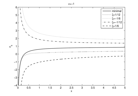
Figure 1: The spectral index versus $x\equiv\frac{\rho_{\varphi}}{\rho_{0}}$ for normal ( $\varepsilon=-1$) branch of the model.

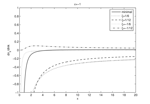
Figure 2: The running of the spectral index versus $x$ for normal branch of the model.

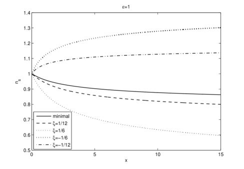
Figure 3: The spectral index versus $x\equiv\frac{\rho_{\varphi}}{\rho_{0}}$ for self-accelerating ( $\varepsilon=+1$) branch of the model.

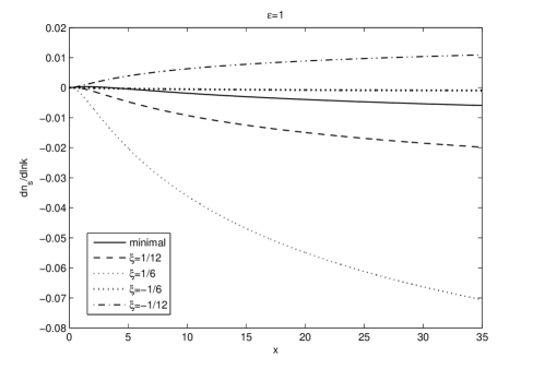
Figure 4: The running of the spectral index versus $x$ for self-accelerating ( $\varepsilon=+1$) branch of the model.

Now we focus on the effect of dissipation on the inflation parameters. Figure 5 shows the variation of the slow-roll parameter $\epsilon$ versus $x$ for different values of the dissipation factor, $r$. As this figure shows, $\epsilon$ decreases by increasing the dissipation effect for a fixed value of $x$.

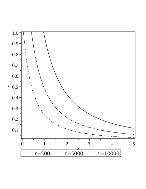
Figure 5: The slow-roll parameter $\epsilon$ versus $x\equiv\frac{\rho_{\varphi}}{\rho_{0}}$ for self-accelerating ( $\varepsilon=+1$) branch of the model for different values of the dissipation factor, $r$.

In figure 6 we have considered the situation for a continuous variation of the dissipation parameter. Again this figure shows that the slow-roll parameter decreases by increasing $r$. However, $\epsilon$ increases by increasing $x$ where $x\equiv\frac{\rho_{\varphi}}{\rho_{0}}$.

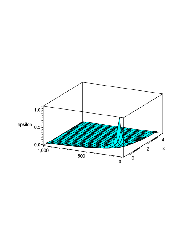
Figure 6: The slow-roll parameter $\epsilon$ versus $x\equiv\frac{\rho_{\varphi}}{\rho_{0}}$ and $r$ for self-accelerating ( $\varepsilon=+1$) branch of the model.

Now to see the effect of dissipation on the number of e-folds, we define

$$g\equiv-\frac{1}{\mu^{2}}\frac{(1+r)}{\Big{(}V_{,\varphi}-\xi f(R)\varphi\Big{)}}\bigg{[}\rho_{\varphi}+\rho_{0}+\varepsilon\rho_{0}\Big{(}{\cal{A}}_{0}^{2}+\frac{2\eta\rho_{\varphi}}{\rho_{0}}\Big{)}^{1/2}\bigg{]}\,,$$ (92)

which is the integrand of the number of e-folds defined as (27). We rephrase this quantity and also equation (27) versus $x$. Figure 7 shows the variation of $g$ versus $x$ for different values of the dissipation factor, $r$. The number of e-folds is given by the surface enclosed between this curve and two vertical lines located at $x_{i}$ and $x_{e}$ corresponding to $\varphi_{i}$ and $\varphi_{e}$ respectively. As this figure shows, the number of e-folds increases by increasing dissipation factor.

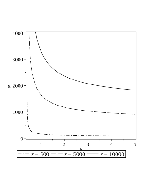
Figure 7: Variation of $g$ versus $x\equiv\frac{\rho_{\varphi}}{\rho_{0}}$ for self-accelerating ( $\varepsilon=+1$) branch of the model for different values of the dissipation factor, $r$.

Finally, we note that the self-accelerating solution of the DGP setup is unstable due to existence of ghosts [51,52]. In our setup, incorporation of several new degrees of freedom such as modified induced gravity, non-minimal coupling and the warped geometry of the bulk has provided a relatively wider parameter space. This wider parameter space may provide a better framework to treat instabilities of the self-accelerating solution. However this is not an easy task and lies out of our interest here ( for a recent progress in this direction see [53]).

8 Summary and Conclusions

In this paper we have studied cosmological perturbations and their evolution in a braneworld viewpoint of the warm inflation in the presence of interaction between inflaton and induced gravity on the brane. We have incorporated possible modification of the induced gravity on the brane in the spirit of $f(R)$-gravity. The cosmological perturbations are treated with complete details and the roles played by modification of the induced gravity, dissipation and the non-minimal coupling are discussed. The main results of our study can be summarized as follows: in the minimal standard theory of cosmological perturbations, when there are no dissipation effects, all perturbations are adiabatic and there is no trace of the non-adiabatic perturbations. But, as we have shown here, in a DGP-inspired non-minimal setup with modified induced gravity, in the absence of dissipation there is a non-vanishing contribution of the non-adiabatic perturbations. In this setup, this effect is mainly as a result of DGP ( with modified induced gravity) than the non-minimal coupling. The effect of the non-minimal coupling tends to increase the contribution of the entropy perturbations. The numerical analysis of the parameter space ( which is wide enough due to incorporation of several new degrees of freedom) shows that it is possible to have both red and blue spectrum and relatively large running of the spectral index depending on the sign of the non-minimal coupling. However, negative values of the non-minimal coupling give results that are not supported by observations and therefore should be excluded from our considerations. The effect of dissipation is so that the slow-roll parameter $\epsilon$ decreases by increasing the dissipation factor. However, the number of e-folds increases by increasing the dissipation factor. Modification of the induced gravity and its coupling to the inflaton field in a warm inflation framework brings a variety of new possibilities which constraint our model in comparison with the recent observations. In other words, this wider parameter space provides much more freedom than single, self-interacting scalar field inflation to fit with the observational data.

9 Acknowledgments

We are indebted to an anonymous referee for insightful suggestions and comments. Part of this work has been done during B. F. sabbatical leave at the INFN Institute, Frascati, Italy. She would like to express her deepest appreciation to the members of this Institute, especially Professor Stefano Bellucci for kind hospitality and supports. The work of K. N. is supported financially by the Research Institute for Astronomy and Astrophysics of Maragha, Iran.

References

- [1] A. Liddle and D. Lyth, Cosmological Inflation and Large-Scale Structure, Cambridge University Press, 2000.
- [2] R. H. Brandenberger, [arXiv:hep-th/0509099]; B. A. Bassett, S. Tsujikawa and D. Wands, Rev. Mod. Phys. 78, 537 (2006), [arXiv:astro-ph/0507632]; J. E. Lidsey et al, Rev. Mod. Phys. 69, 373 (1997).
- [3] A. Berera and L. Z. Fang, Phys. Rev. Lett. 74, 1912 (1995).
- [4] A. Berera, Phys. Rev. Lett. 75, 3218 (1995).
- [5] A. Berera, Phys. Rev. D 54, 2519 (1996).
- [6] A. Berera, Nucl. Phys B 585, 666 (2000), [arXiv:hep-ph/9904409].
- [7] A. Berera, Contemporary Phys. 47, 33 (2006), [arXiv:0809.4198]; A. Berera, I. G. Moss and R. O. Ramos, Rept. Prog. Phys. 72, 026901 (2009), [arXiv:0808.1855]; M. Bastero-Gil and A. Berera, [ arXiv:0902.0521]; A. Berera, M. Gleiser and R. O. Ramos, Phys. Rev. Lett. 83, 264 (1999), [arXiv:hep-ph/9809583]; M. Bellini, Class. Quant. Grav. 16,2393 (1999), [arXiv:gr-qc/9904072]; M. Bellini, Nucl. Phys. B 563, 245 (1999), [ arXiv:gr-qc/9908063]; S. Gupta, A. Berera, A. F. Heavens and S. Matarrese, Phys. Rev. D 66, 043510 (2002), [arXiv:astro-ph/0205152]; R. H. Brandenberger and M. Yamaguchi, Phys. Rev. D 68, 023505 (2003), [arXiv:hep-ph/0301270]; L. M. H. Hall, Ian G. Moss and A. Berera, Phys. Rev. D 69, 083525 (2004), [arXiv:astro-ph/0305015]; L. M. H. Hall, I. G. Moss and A. Berera, Phys. Lett. B 589, 1 (2004), [ arXiv:astro-ph/0402299]; S. Gupta, Phys. Rev. D 73, 083514 (2006), [arXiv:astro-ph/0509676]; A. Berera, Grav. Cosmol. 11, 51 (2005), [ arXiv:hep-ph/0604124]; M. Bastero-Gil and A. Berera, [arXiv:hep-ph/0610343]; J. C. Bueno Sanchez, M. Bastero-Gil, A. Berera and K. Dimopoulos, [arXiv:0802.4354]; A. Berera, Contemporary Physics 47, 33 (2006), [arXiv:0809.4198]; A. Berera, I. G. Moss and R. O. Ramos, [arXiv:0808.1855]; I. G Moss and C. Xiong, [arXiv:0808.0261]; J. M. Romero and M. Bellini, Nuovo Cim. B 124 (2009) 861; R. Herrera, [arXiv:1006.1299].
- [8] I. G. Moss, Phys. Letts. B 154, 120 (1985).
- [9] A. Berera, Phys. Rev. D 55, 3346 (1997).
- [10] G. Dvali, G. Gabadadze and M. Porrati, Phys. Lett. B 485, 208 (2000) , [arXiv:hep-th/0005016].
- [11] A. Lue, Physics Reports 423, 1 (2006) [arXiv:astro-ph/0510068].
- [12] Kei-ichi Maeda, S. Mizuno and T. Torii, Phys. Rev. D 68, 024033 (2003), [arXiv:gr-qc/0303039].
- [13] R. -G. Cai and H. Zhang, JCAP 0408, 017 (2004), [arXiv:hep-th/0403234].
- [14] M. Bouhamdi-Lopez, R. Maartens and D. Wands, Phys. Rev. D 70, 123519 (2004), [arXiv:hep-th/0407162].
- [15] E. Papantonopoulos and V. Zamarias, JCAP 0410, 001 (2004), [ arXiv:gr-qc/0403090].
- [16] H. Zhang and Z. Zhu, Phys. Lett. B 641, 405 (2006), [arXiv:astro-ph/0602579].
- [17] K. Nozari and B. Fazlpour, JCAP 11, 006 (2007), [arXiv:0708.1916].
- [18] S. del Campo and R. Herrera, Phys. Lett. B 653, 122 (2007), [arXiv:gr-qc/0708.1460].
- [19] V. Faraoni, Phys. Rev. D 53, 6813 (1996); V. Faraoni, Phys. Rev. D 62, 023504 (2000), [arXiv:gr-qc/0002091].
- [20] R. H. Brandenberger, [arXiv:astro-ph/9711106]. See also R. H. Brandenberger, Lect. Notes Phys. 738, 393 (2008), [arXiv:hep-th/0701111]; R. H. Brandenberger and X. Zhang, [arXiv:0903.2065].
- [21] T. P. Sotiriou and V. Faraoni, [arXiv:gr-qc/0805.1726]. For inflation in the spirit of modified gravity, see for instance B. Chen, M. Li, T. Wang and Y. Wang, Mod. Phys. Lett. A 22 , 1987 (2007), [arXiv:astro-ph/0610514], G. Cognola, E. Elizalde, S. Nojiri, S.D. Odintsov, L. Sebastiani and S. Zerbini, Phys. Rev. D 77, 046009 (2008), [arXiv:0712.4017]; See also S. Nojiri and S. D. Odintsov, Phys. Rev. D 68, 123512 (2003), [arXiv:hep-th/0307288].
- [22] J. W. York, Phys. Rev. Lett. 28, 1082 (1972); G. W. Gibbons and S. W. Hawking, Phys. Rev. D 15, 2752 (1977). See also R. Dick, Class. Quant. Grav. 18, R1 (2001), [arXiv:hep-th/0105320].
- [23] L. Randall and R. Sundrum, Phys. Rev. Lett. 83, 4690 (1999).
- [24] B. Gumjudpai, R. Maartens and C. Gordon, Class. Quant. Grav. 20, 3295 (2003), [ arXiv:gr-qc/0304067]. See also R. Maartens, [arXiv:astro-ph/0402485].
- [25] S. Nojiri and S. D. Odintsov, Phys. Lett. B 599, 137 (2004), [arXiv:astro-ph/0403622]; S. Nojiri, S. D. Odintsov, P. V. Tretyakov, Prog. Theor. Phys. Suppl. 172, 81 (2008), [arXiv:0710.5232];
- [26] Y. Zhang, [ arXiv:0903.0685].
- [27] M. Szydlowski, O. Hrycyna and A. Kurek, Phys. Rev. D 77, 027302 (2008) [arXiv:0710.0366].
- [28] V. F. Mukhanov, H. A. Feldman and R. H. Brandenberger, Phys. Rep. 215, 203 (1992).
- [29] J. Bardeen, Phys. Rev. D 22, 1882 (1980).
- [30] A. Riotto, [arXiv:hep-ph/0210162].
- [31] K. Nozari, JCAP 09, 003 (2007), [arXiv:0708.1611].
- [32] H. P. De Oliveira and S. E. Joras, Phys. Rev. D 64, 063513 (2001), [arXiv:gr-qc/0103089].
-
[33]
K. Koyama and R. Maartens, JCAP 0601, 016 (2006),
[arXiv:astro-ph/0511634]
D. Langlois, R. Maartens, M. Sasaki and D. Wands, Phys. Rev. D 63 (2001) 084009 - [34] C. Gordon, D. Wands, B. A. Bassett and R. Maartens, Phys. Rev. D 63, 023506 (2001), [arXiv:astro-ph/0009131].
- [35] D. Langlois and F. Vernizzi, JCAP 02, 017 (2007), [arXiv:astro-ph/0610064].
- [36] N. Bartolo, S. Matarrese and A. Riotto, Phys. Rev. D 64, 083514 (2001).
- [37] N. Bartolo, S. Matarrese and A. Riotto, Phys. Rev. D 64, 123504 (2001).
- [38] N. Bartolo, S. Matarrese, A. Riotto and D. Wands, Phys. Rev. D 66, 043520 (2002).
- [39] H. P. de Oliveira, Phys. Lett. B 526,1 (2002).
- [40] A. A. Starobinsky and J. Yokoyama, [arXiv:gr-qc/9502002]; A. A. Starobinsky, S. Tsujikawa and J. Yokoyama, Nucl. Phys. B 610,383 (2001).
- [41] H. Kodama and M. Sasaki, Prog. Theor. Phys. Supp. 78, 1 (1984).
- [42] B. A. Bassett, F. Tamburini, D. I. Kaiser and R. Maartens, Nucl.Phys. B 561, 188-240(1999), [arXiv:hep-ph/9901319]; C. Gordon, D. Wands, B. A. Basset and R. Maartens, Phys. Rev. D 63, 023506 (2001), [arXiv:astro-ph/0009131].
- [43] D. Polarski and A. A. Starobinsky, Nucl. Phys. B 385, 623 (1992).
- [44] D. Wands, K. A. Malik, D. H. Lyth and A. R. Liddle, Phys. Rev. D 62, 043527 (2000).
- [45] A. R. Liddle and A. Mazumdar, Phys. Rev. D61 (2000) 123507 ; M. A. Cid, S. D. Campo and R. Herrera, JCAP 10, 005 (2007), [arXiv:astro-ph/0710.3148].
- [46] A. N. Taylor and A. Berera, Phys. Rev. D 62, 083517 (2000).
- [47] Y. -Z. Ma and X. Zhang, JCAP 03, 006 (2009), [arXiv:0812.3421].
- [48] K. Bhattacharya, S. Mohanty and A. Nautiyal, Phys. Rev. Lett. 97, 251301 (2006), [arXiv:astro-ph/0607049].
- [49] E. Komatsu et al., Astrophys. J. Suppl. 180, 330 (2009), [arXiv:0803.0547].
- [50] G. Cognola, E. Elizalde, S. Nojiri, S. D. Odintsov and S. Zerbini, Phys. Rev. D 73, 084007 (2006), [arXiv:hep-th/0601008]; See also S. Nojiri and S. D. Odintsov, Int. J. Geom. Meth. Mod. Phys. 4, 115 (2007), [arXiv:hep-th/0601213].
- [51] K. Koyama, Class. Quantum Grav. 24, R231 (2007) [arXiv:hep-th/0709.2399].
- [52] C. de Rham and A. J. Tolley, JCAP 0607, 004 (2006) [arXiv:hep-th/0605122].
- [53] See for instance: M. Sami, [arXiv:0904.3445]; M. Cadoni and P. Pani, [arXiv:0812.3010]; Y. Shtanov, V. Sahni, A. Shafieloo and A. Toporensky, JCAP 04 (2009) 023, [arXiv:0901.3074].