Consistent estimation of non-bandlimited spectral density from uniformly spaced samples

Abstract

In the matter of selection of sample time points for the estimation of the power spectral density of a continuous time stationary stochastic process, irregular sampling schemes such as Poisson sampling are often preferred over regular (uniform) sampling. A major reason for this preference is the well-known problem of inconsistency of estimators based on regular sampling, when the underlying power spectral density is not bandlimited. It is argued in this paper that, in consideration of a large sample property like consistency, it is natural to allow the sampling rate to go to infinity as the sample size goes to infinity. Through appropriate asymptotic calculations under this scenario, it is shown that the smoothed periodogram based on regularly spaced data is a consistent estimator of the spectral density, even when the latter is not band-limited. It transpires that, under similar assumptions, the estimators based on uniformly sampled and Poisson-sampled data have about the same rate of convergence. Apart from providing this reassuring message, the paper also gives a guideline for practitioners regarding appropriate choice of the sampling rate. Theoretical calculations for large samples and Monte-Carlo simulations for small samples indicate that the smoothed periodogram based on uniformly sampled data have less variance and more bias than its counterpart based on Poisson sampled data.

I Introduction

Estimation of the power spectral density of a continuous time wide sense stationary stochastic process is an old problem. A set of regularly (uniformly) spaced samples is generally used for this purpose. When the process is bandlimited, the spectral density of the original process can be recovered from that of the sampled process, provided that the sampling is fast enough. In such a case, estimation of the spectral density from finitely many observations at an appropriate sampling rate is a well established topic and many useful nonparametric and parametric methods have been developed [1]. If the underlying process is not bandlimited, the spectral density of the original process is not identifiable from regularly spaced samples, because of the problem of wrapping around of the spectral density caused by the process of sampling – also known as aliasing [2]. In such a case, one cannot estimate the spectral density consistently from regularly spaced samples at any fixed sampling rate.

This inadequacy of sampling at regular intervals necessitated the exploration of other strategies for sampling. Shapiro and Silverman [3] considered alias free sampling schemes in the sense that two continuous time processes with different power spectra do not produce the same spectrum of the sampled sequence. They proved that additive random sampling through a class of renewal processes, including the homogeneous Poisson process, is alias free. Beutler [4] formalized the definition of alias free sampling relative to a family of spectral distributions and gave different sampling schemes that are alias free relative to different families of spectral distributions. Masry [5] provided a modified definition of alias free sampling that would guarantee the existence of a consistent estimator of the power spectral density.

Subsequently, the possibility of breaking free from the nuisance of aliasing through irregular sampling enthused many researchers and practitioners. Masry [6] proposed a Poisson sampling based estimator similar to the smoothed periodogram, and proved that the proposed estimator is consistent for any average sampling rate, under certain conditions. Several irregular sampling based methodologies of estimation of the power spectral density of a non-bandlimited process have also been proposed [7]–[11] and applied to various fields including signal and image processing. Some of these methods are analogous to methods developed for regularly sampled data.

Irregularly spaced data occur naturally in many practical situations like seismic data [12], turbulent velocity fluctuation [13], Laser Doppler Anemometer (LAD) data [14], wide-band antenna arrays [15], Computer Aided Tomography, Spotlight-Mode Synthetic Aperture Radar [16] and so on. There have been attempts to use standard methods for spectrum estimation for such data, after suitable weighting[17] or interpolation [13] of the data. The advent of new methodologies for irregularly sampled data are important for such problems.

However, in many applications, including internet traffic data [18], seismology [19], [20], image processing [21] and so on, one has control over the sampling mechanism. In such cases, the selection of the sampling scheme is a serious issue. Regular sampling is easier to implement than irregular sampling. The literature on power spectrum estimation based on regular sampling contains a large collection of methods, and these have been studied in detail. An estimator based on regularly sampled data is generally computationally simpler than a similar estimator based on irregularly sampled data. Moreover, it is well known that spectral estimators based on irregularly sampled data have higher variances than those based on regularly sampled data [22], [23]. On the other hand, the possibility of aliasing and the proven inconsistency of spectral estimators based on regular sampling are arguments in favour of using irregular sampling.

These opposing arguments necessitate a thorough comparison of spectral estimators based on different sampling strategies. A systematic numerical comparison is not available in the literature. A simulated example given by Masry [24] was meant only to highlight the problem of aliasing and to demonstrate how it can be overcome with irregular sampling. Studies by Roughan [18] in the special case of active measurements for network performance produced mixed results, which led the author to conclude that, while spectral estimators based on Poisson sampling have less efficiency (i.e., high variance), such techniques could be used to detect periodicities in the system, and to determine which rate of regular sampling would be inadequate. In the absence of a comprehensive empirical study, it appears that many researchers shun regular sampling mainly because of the stigma of inconsistency attached to spectral estimators based on regularly sampled data [25].

Consistency of an estimator concerns its behaviour as the sample size goes to infinity. However, it does not make practical sense to let the sample size tend to infinity with fixed sampling rate. If one gathers more and more resources to increase the sample size, one can use some of these resources to sample faster. Realizing this, practitioners fix the intended range of spectrum estimation, and then sample an appropriately filtered process at a sufficiently high frequency to avoid aliasing. Sometimes one goes for successively higher rates of uniform sampling to determine an appropriate rate of sampling [21]. However, these common sense approaches are yet to be backed up by appropriate asymptotic calculations. There is a need to bridge this gap by working out the large sample properties of estimators when the sampling rate changes suitably as the sample size goes to infinity.

Let $\phi(\cdot)$ be the spectral density of a mean square continuous, wide sense stationary process $\{X(t),\ -\infty<t<\infty\}$. The most commonly used nonparametric estimator of $\phi(\cdot)$ based on the $n$ uniformly spaced samples at the sampling rate $\rho$ is $\widehat{\phi}_{\rho}(\cdot)$, where

$$\widehat{\phi}_{\rho}(\lambda)=\frac{1}{2\pi\rho}\sum_{|v|<n}\widehat{\gamma}_{\rho}(v)K(b_{n}v)e^{-\frac{iv\lambda}{\rho}}1_{[-\pi\rho,\pi\rho]}(\lambda),$$ (I.1)

where $K(\cdot)$ is a covariance averaging kernel, $1_{A}(\lambda)$ is the indicator function that takes the value 1 when $\lambda\in A$ and the value 0 otherwise, $\{b_{n}\}$ is a sequence of window widths such that $b_{n}\rightarrow 0$ and $nb_{n}\rightarrow\infty$ as ${n\rightarrow\infty}$ and $\widehat{\gamma}_{\rho}(v)$ is an estimator of the covariance function, defined as

$$\begin{split}\widehat{\gamma}_{\rho}(v)=&\frac{1}{n}\sum_{j=1}^{n-|v|}X\left(\frac{j}{\rho}\right)X\left(\frac{j+|v|}{\rho}\right),\\ &\hskip 43.36243ptv=-(n-1),-(n-2),\ldots,n-2,n-1.\end{split}$$

This estimator is known to be consistent when the underlying process is bandlimited.

In the present work, without assuming that the process is bandlimited, we examine the asymptotic properties of the estimator given in (I.1) by letting $\rho$ go to infinity at an appropriate rate, as $n$ goes to infinity. In the sequel, we shall use the notation $\rho_{n}$ instead of $\rho$, in order to explicitly indicate the dependence of the sampling rate on the sample size. Accordingly, we use the following modified notation of the estimator of (I.1):

$$\widehat{\phi}_{n}(\lambda)=\frac{1}{2\pi\rho_{n}}\sum_{|v|<n}\widehat{\gamma}_{n}(v)K(b_{n}v)e^{-\frac{iv\lambda}{\rho_{n}}}1_{[-\pi\rho_{n},\pi\rho_{n}]}(\lambda)$$ (I.2)

where

$$\begin{split}\widehat{\gamma}_{n}(v)=&\frac{1}{n}\sum_{j=1}^{n-|v|}X\left(\frac{j}{\rho_{n}}\right)X\left(\frac{j+|v|}{\rho_{n}}\right),\\ &\hskip 43.36243ptv=-(n-1),-(n-2),\ldots,n-2,n-1.\end{split}$$ (I.3)

In Section II, we prove the consistency of the estimator $\widehat{\phi}_{n}(\cdot)$ under some general conditions. In Section III, we calculate the rate of convergence of the bias and variance of this estimator, and determine the optimal rates at which $\rho_{n}$ and $nb_{n}$ should go to infinity so that the mean square error has the fastest possible rate of convergence. Subsequently, we compare the rates of convergence of the bias and the mean squared error (MSE) of this estimator with those of a similar estimator proposed by Masry [6], based on non-uniform (Poisson) sampling. We present the results of a simulation study in Section IV and provide some concluding remarks in Section V. The proofs are given in the appendix.

II Consistency of the estimator

Consider the mean square continuous, wide sense stationary stochastic process $\{X(t),~{}-\infty<t<\infty\}$ with zero mean, (auto-)covariance function $C(\cdot)$ and spectral density $\phi(\cdot)$. In order to prove that the estimator (I.2) is consistent, it is sufficient to show that the bias and the variance of the estimator tend to zero as the sample size ($n$) tends to infinity.

We assume the following condition on the covariance function $C(\cdot)$.

Condition 1. The function $h_{0}(\cdot)$, defined over the real line as $h_{0}(t)=\sup_{s\geq|t|}|C(s)|$ is integrable.

Remark 1. Condition 1 is equivalent to saying that the covariance function $C(\cdot)$ is bounded over $[0,\infty)$ by a non-negative, non-increasing and integrable function.

We assume the following conditions on the choice of the kernel $K(\cdot)$, the kernel window width $b_{n}$ and the sampling rate $\rho_{n}$.

Condition 2. The covariance averaging kernel function $K(\cdot)$ is continuous, even, square integrable and bounded by a non-negative, even and integrable function having a unique maximum at 0. Further, $K(0)=1$.

Condition 3. The kernel window width is such that $b_{n}\rightarrow 0$ and $nb_{n}\rightarrow\infty$ as $n\rightarrow\infty$.

Condition 4. The sampling rate is such that $\rho_{n}\rightarrow\infty$ and $\rho_{n}b_{n}\rightarrow 0$ as $n\rightarrow\infty$.

Remark 2. Note that the estimator $\widehat{\phi}_{n}(\cdot)$ can be written as

$$\widehat{\phi}_{n}(\lambda)={1\over\rho_{n}b_{n}}\int_{-\infty}^{\infty}I_{n}(\mu)W_{n}\left({\lambda-\mu\over\rho_{n}b_{n}}\right)d\mu,$$

where

$$I_{n}(\lambda) = \frac{1}{2\pi n\rho_{n}}\left|\sum_{t=1}^{n}X\!\left(\frac{t}{\rho_{n}}\right)e^{-\frac{it\lambda}{\rho_{n}}}\right|^{2}1_{[-\pi\rho_{n},\pi\rho_{n}]}(\lambda),$$

$$W_{n}(\lambda) = \sum_{j=-\infty}^{\infty}\int_{-\infty}^{\infty}K(t)e^{-\frac{it\lambda}{\rho_{n}}-2\pi ijt}dt.$$

Thus, $\widehat{\phi}_{n}(\cdot)$ is the smoothed version of $I_{n}(\cdot)$, the periodogram, where the degree of smoothness is controlled by the smoothing parameter $\rho_{n}b_{n}$ of the frequency domain window $W_{n}(\cdot)$. Condition 4 says that this parameter goes to zero, and the sampling rate goes to infinity, as the sample size goes to infinity.

Theorem 1.

Under Conditions 1–4, the bias of the estimator $\widehat{\phi}_{n}(\cdot)$ given by (I.2) tends to zero uniformly over any closed and finite interval.

Before examining the variance of the estimator we assume the following condition on the fourth order moments of the process $\{X(t),~{}-\infty<t<\infty\}$.

Condition 5. The fourth moment $E|X(t)|^{4}$ exists for every $t$, and the fourth moment function $E[X(t)X(t+v_{1})X(t+v_{2})X(t+v_{3})]$ is a function only of the lags $v_{1}$, $v_{2}$ and $v_{3}$. Further, the fourth order cumulant function $Q(v_{1},v_{2},v_{3})$, defined by

$$Q(v_{1},v_{2},v_{3}) = P(v_{1},v_{2},v_{3})-P_{G}(v_{1},v_{2},v_{3}),$$

where

$$P(v_{1},v_{2},v_{3}) = E(X(t)X(t+v_{1}))X(t+v_{2})X(t+v_{3})$$

$$\mbox{and }P_{G}(v_{1},v_{2},v_{3}) = C(v_{1})C(v_{2}-v_{1})+C(v_{2})C(v_{3}-v_{1})$$

$$+C(v_{3})C(v_{1}-v_{2}),$$

satisfies

$$|Q(v_{1},v_{2},v_{3})|\leq\prod_{i=1}^{3}g_{i}(v_{i}),$$

where $g_{i}(v),\ i=1,2,3,$ are all continuous, even, nonnegative and integrable functions over the real line, which are non-increasing over $[0,\infty)$.

Remark 3. Condition 5 is satisfied by a Gaussian process, as the function $P(\cdot)$ reduces to the function $P_{G}(\cdot)$.

Theorem 2.

Under Conditions 1–5, the variance of the estimator $\widehat{\phi}_{n}(\cdot)$ given by (I.2) converges as follows:

$$\lim_{n\rightarrow\infty}nb_{n}Var[\widehat{\phi}_{n}(\lambda)]=(1+\delta_{0,\lambda})[\phi(\lambda)]^{2}\int_{-\infty}^{\infty}K^{2}(x)dx,$$

where $\delta_{0,\lambda}$ is 1 if $\lambda=0$ and is 0 otherwise. The convergence is uniform over any closed and finite interval that does not include the frequency 0. In particular, the variance converges to 0.

It follows from Theorems 1 and 2 that, under Conditions 1–5, the estimator $\widehat{\phi}_{n}(\lambda)$ is consistent, and is uniformly consistent over any closed and finite frequency interval that does not include the point 0.

III Rates of Convergence

The rate of convergence of the variance of $\widehat{\phi}_{n}(\lambda)$ follows from Theorem 2. We assume a few further conditions in order to arrive at a rate of convergence for its bias. These include additional conditions on the shapes of the covariance function and the kernel function.

Condition 1A. The function $h_{q}(\cdot)$, defined over the real line as $h_{q}(t)=\sup_{s\geq|t|}|s|^{q}|C(s)|$ is integrable, for some positive number $q$ greater than 1.

Condition 1B. The spectral density is such that, for some $p>1$, $\phi(\lambda)$ is $O(|\lambda|^{-p})$, i.e., $\displaystyle\lim_{\lambda\rightarrow\infty}|\lambda|^{p}\phi(\lambda)=A$ for some positive $A$.

For any kernel $K(\cdot)$, let us define

$$k_{r}=\lim_{x\rightarrow 0}\frac{1-K(x)}{|x|^{r}}$$

for each positive number $r$ such that the limit exists. The characteristic exponent of the kernel is defined as the largest number $r$, such that the limit exists and is non-zero [26]. In other words, the characteristic exponent is the number $r$ such that $1\!-\!K(1/y)$ is $O(y^{-r})$.

Condition 2A. The characteristic exponent of the kernel $K(\cdot)$ is equal to the number $q$, for which Condition 1A is assumed to hold.

Remark 4. Condition 1A implies Condition 1 (see Remark 1), and also that $\phi(\cdot)$ is $[q]$ times differentiable, where $[q]$ is the integer part of $q$. Thus, the number $q$ indicates the degree of smoothness of the spectral density. If Condition 1A holds for a particular value of $q$, then it would also hold for smaller values.

Remark 5. The number $p$ indicates the rate of decay of the spectral density. The following are two interesting situations, where Condition 1B holds.

1. The spectral density $\phi(\cdot)$ is a rational function, i.e., $\phi(\lambda)=\frac{P(\lambda)}{Q(\lambda)}$, where $P(\cdot)$ and $Q(\cdot)$ are polynomials such that the degree of $Q(\cdot)$ is more than degree of $P(\cdot)$ by at least $p$. Note that continuous time ARMA processes possess rational power spectral density.

2. The function $C(\cdot)$ has the following smoothness property: $C(\cdot)$ is $p$ times differentiable and the $p^{\rm th}$ derivative of $C(\cdot)$ is in $L^{1}$.

Remark 6. The number $p$ can be increased indefinitely by continuous time low pass filtering with a cut off frequency larger than the maximum frequency of interest. There are well-known filters such as the Butterworth filter, which have polynomial rate of decay of the transfer function with specified degree of the polynomial, that can be used for this purpose.

Theorem 3.

Under Condition 2–4, 1A, 1B and 2A, the bias of the estimator $\widehat{\phi}_{n}(\lambda)$ given by (I.2) is

$$\begin{split}&\hskip-7.0ptE[\widehat{\phi}_{n}(\lambda)-\phi(\lambda)]\\ &=\left[-\frac{k_{q}}{2\pi}\int_{-\infty}^{\infty}|t|^{q}C(t)e^{-it\lambda}dt\right](\rho_{n}b_{n})^{q}+o\left((\rho_{n}b_{n})^{q}\right)\\ &~{}+\left[-\frac{1}{2\pi}\int_{-\infty}^{\infty}|t|C(t)e^{-it\lambda}dt\right]\left(\frac{\rho_{n}}{n}\right)+o\left(\frac{\rho_{n}}{n}\right)\\ &~{}+\left[\frac{A}{(2\pi)^{p}}\sum_{|l|>0}\frac{1}{|l|^{p}}\right]\frac{1}{(\rho_{n})^{p}}+o\left(\frac{1}{(\rho_{n})^{p}}\right),\end{split}$$

i.e.,

$$E[\widehat{\phi}_{n}(\lambda)-\phi(\lambda)]=O\left((\rho_{n}b_{n})^{q}\right)+O\left(\frac{\rho_{n}}{n}\right)+O\left(\frac{1}{\rho_{n}^{p}}\right),$$

uniformly in $\lambda$ over any closed and finite interval.

Remark 7. Condition 2A can be relaxed to the extent that the characteristic exponent of the kernel $K(\cdot)$ is required to be greater than or equal to the number $q$, for which Condition 1A is assumed to hold. If it is strictly greater than $q$, then the term $O\left((\rho_{n}b_{n})^{q}\right)$ in the above theorem would have to be replaced by $o\left((\rho_{n}b_{n})^{q}\right)$. This follows from equation (A.17) in the appendix and the fact that $k_{q}=0$ in this case. On the other hand, if a kernel with characteristic exponent less than $q$ is used, then one does not fully utilize the strength of the assumption on the smoothness of the spectral density, implied by Condition 1A, and hence gets a slower rate of convergence.

III-A Choice of $\rho_{n}$ and $b_{n}$

From Theorem 3 and Theorem 2, it is observed that the bias and the variance of the estimator $\widehat{\phi}_{n}(\lambda)$ converge to zero at different rates. We set out to choose the sampling rate $\rho_{n}$ and the window width $b_{n}$ in order to ensure that MSE of $\widehat{\phi}_{n}(\lambda)$ converges to zero as fast as possible. It would turn out that this happens when the squared bias and the variance go to zero at the same rate.

Theorem 4.

Under Conditions 2–5, 1A, 1B and 2A, the optimal rate of convergence of the MSE of the estimator $\widehat{\phi}_{n}(\lambda)$ is given by

$$MSE[\widehat{\phi}_{n}(\lambda)]=O\left(n^{-\frac{2pq}{p+q+2pq}}\right),$$ (III.1)

which corresponds to the optimal choices

$$\rho_{n} = P~{}n^{\frac{q}{p+q+2pq}},$$ (III.2)

$$\mbox{and }b_{n} = Q~{}n^{-\frac{p+q}{p+q+2pq}},$$ (III.3)

for some positive constants $P$ and $Q$.

The above optimal rates of $\rho_{n}$ and $b_{n}$ lead to the following corollaries to Theorems 2 and 3, respectively.

Corollary 1. Under the Conditions 1, 2, 5 and the choices of $\rho_{n}$ and $b_{n}$ given by (III.2–III.3), we have

$$\lim_{n\rightarrow\infty}n^{\frac{2pq}{p+q+2pq}}Var[\widehat{\phi}(\lambda)]=\frac{1}{Q}(1+\delta_{0,\lambda})[\phi(\lambda)]^{2}\int_{-\infty}^{\infty}K^{2}(x)dx,\qquad$$ (III.4)

where $\delta_{0,\lambda}$ is equal to 1 if $\lambda=0$, and is 0 otherwise.

Corollary 2. Under the Conditions 1A, 1B, 2, 2A and the choices of $\rho_{n}$ and $b_{n}$ given by (III.2–III.3), we have

$$\begin{split}&\hskip-15.0pt\lim_{n\rightarrow\infty}n^{\frac{pq}{p+q+2pq}}E[\widehat{\phi}_{n}(\lambda)-\phi(\lambda)]\\ =&-(PQ)^{q}\frac{k_{q}}{2\pi}\int_{-\infty}^{\infty}|t|^{q}C(t)e^{-it\lambda}dt\!+\!\frac{1}{P^{p}}\frac{A}{(2\pi)^{p}}\sum_{|l|>0}\frac{1}{|l|^{p}},\end{split}$$ (III.5)

where the constant $A$ is as in Condition 1B.

III-B Comparison with Poisson Sampling

Among the various schemes for sampling a continuous time stochastic process at irregular intervals, the Poisson sampling proposed by Silverman [3] is the simplest and most popular. Here, we compare the asymptotic behaviour of the estimator $\widehat{\phi}_{n}(\cdot)$ with a similar estimator based on Poisson sampling.

Let $\{t_{j}\}_{j=0}^{n}$ be the sampling points from a Poisson process with average sampling rate $\rho$. Masry [6] proved that, under Conditions 1, 2, 3 and 5, the estimator $\widehat{\psi}_{n}(\cdot)$ defined as

$$\begin{split}&\hskip-7.0pt\widehat{\psi}_{n}(\lambda)\\ =&\frac{1}{\pi\rho n}\sum_{i=1}^{n-1}\sum_{j=1}^{n-i}X(t_{j})X(t_{j+i})K(b_{n}(t_{j+i}\!-\!t_{j}))\cos(\lambda(t_{j+i}\!-\!t_{j})),\end{split}$$

is consistent for $\phi(\lambda)$ for any choice of $\rho$.

Under the above conditions, the asymptotic variance of $\widehat{\psi}_{n}(\lambda)$ satisfies

$$\begin{split}&\hskip-25.0pt\lim_{n\rightarrow\infty}(nb_{n})Var[\widehat{\psi}_{n}(\lambda)]\\ =&\rho\left[\phi(\lambda)+\frac{C(0)}{2\pi\rho}\right]^{2}(1+\delta_{0,\lambda})\int_{-\infty}^{\infty}K^{2}(t)dt.\end{split}$$ (III.6)

For specifying the rate of convergence of the bias, Masry [6] assumed the following additional conditions.

Condition 1C. $|t|^{q}C(t)$ is integrable for some positive integer $q$.

Condition 2B. $K(\cdot)$ is $q$ times differentiable with bounded derivatives, where $q$ is an integer for which Condition 1C holds.

Note that Condition 1C is implied by Condition 1A with the same or higher value of $q$ as is used here. Masry [6] showed that, under Conditions 1, 2, 3, 1C and 2B, the bias of the estimator $\widehat{\psi}_{n}(\lambda)$ is given as

$$\begin{split}Bias[\widehat{\psi}_{n}(\lambda)]=&E[\widehat{\psi}_{n}(\lambda)]-\phi(\lambda)\\ =&\sum_{l=1}^{q-1}\frac{(i)^{l}K^{(l)}(0)b_{n}^{l}}{l!}\phi^{(l)}(\lambda)+O(b_{n}^{q})+O\left(\frac{1}{n}\right).\end{split}$$ (III.7)

It follows from (III.7) that the rate of convergence of the bias of $\widehat{\psi}_{n}(\lambda)$ is $O\left(\max\left\{b_{n}^{m},n^{-1}\right\}\right)$, where

$$m=\begin{cases}q&\mbox{if $K^{(l)}(0)=0$ for $1\leq l<q$},\\ l_{0}&\mbox{if $K^{(l_{0})}(0)\neq 0$ and $K^{(l)}(0)=0$ for $1\!\leq\!l\!<\!l_{0}\!<\!q$}.\\ \end{cases}$$

The fastest possible rate of convergence is $O\left(\max\left\{b_{n}^{q},n^{-1}\right\}\right)$, and this is achieved when one uses a kernel, which further satisfies Condition 2A with the same or higher value of $q$ as is used here. In such a case, we have

$$Bias[\widehat{\psi}_{n}(\lambda)]=O(b_{n}^{q})+O\left(\frac{1}{n}\right).$$ (III.8)

If the condition 2A holds with a higher value of $q$, then the term $O(b_{n}^{q})$ has to be replaced by $o(b_{n}^{q})$

Let us now assume that the kernel is chosen appropriately to ensure (III.8). Note that the bias and the variance of $\widehat{\psi}_{n}(\lambda)$ converge to zero at different rates. One can choose the rate of convergence of the window width $b_{n}$ such that the MSE converges as fast as possible. It turns out that if $b_{n}=O(n^{-\alpha})$, then the optimal choice of $\alpha$ is $\frac{1}{2q+1}$, in which case the squared bias and variance of $\widehat{\psi}_{n}(\lambda)$ are both $O(n^{-\frac{2q}{2q+1}})$.

In summary, under Conditions 1, 1C, 2, 2A, 2B, 5 and

$$b_{n}=R~{}n^{-\frac{1}{2q+1}},$$ (III.9)

the MSE of $\widehat{\psi}_{n}(\lambda)$ is

$$MSE[\widehat{\psi}_{n}(\lambda)]=O\left(n^{-\frac{2q}{2q+1}}\right).$$

The rate of convergence of MSE of $\widehat{\phi}_{n}(\lambda)$ is given in Theorem 4 under Conditions 1A, 1B, 2, 2A, 5 and (III.2–III.3). Both the results hold when $\rho_{n}$ and $b_{n}$ for $\widehat{\phi}_{n}(\cdot)$ are chosen as in (III.2–III.3), $b_{n}$ for $\widehat{\psi}_{n}(\cdot)$ is chosen as in (III.9) and the following conditions hold simultaneously: Condition 1A for some $q$ greater than 1 (which implies Condition 1C for $[q]$ and Condition 1), Condition 2, Condition 2A (for the same $q$ as in Condition 1A), condition 2B for $[q]$, and Condition 5. Under this common set of conditions, we have

$$MSE[\widehat{\psi}_{n}(\lambda)] =O\left(n^{-\frac{2[q]}{2[q]+1}}\right),$$

$$MSE[\widehat{\phi}_{n}(\lambda)] =O\left(n^{-\frac{2q}{2q+1+q/p}}\right).$$

When $q$ is an integer, i.e., $[q]=q$, the rate of convergence of the MSE of $\widehat{\phi}_{n}(\lambda)$ is slower than that of $\widehat{\psi}_{n}(\lambda)$. The two rates are comparable if $p$ is much larger than $q$. When $q$ is not an integer, the MSE of $\widehat{\phi}_{n}(\lambda)$ converges faster when $p>q[q]/(q-[q])$, and in particular when $p$ is very large. As we have indicated in Remark 6, for every fixed $q$, one can make $p$ suitably large through low pass filtering.

If the rates of convergence are comparable, the constants associated with these rates become important. We will compare the constants of the asymptotic bias of $\widehat{\phi}_{n}(\lambda)$ and $\widehat{\psi}_{n}(\lambda)$ as well as the constants of their asymptotic variance separately, assuming that $q$ is an integer.

Under Conditions 1, 2, 5 and (III.9), we have

$$\begin{split}&\hskip-22.0pt\lim_{n\rightarrow\infty}n^{\frac{2q}{2q+1}}Var[\widehat{\psi}_{n}(\lambda)]\\ =&\frac{1}{R}\rho\left[\phi(\lambda)+\frac{C(0)}{2\pi\rho}\right]^{2}(1+\delta_{0,\lambda})\int_{-\infty}^{\infty}K^{2}(x)dx.\end{split}$$ (III.10)

On the other hand, we have from Corollary 1 that under the Conditions 1, 2, 5 and (III.2–III.3),

$$\begin{split}&\hskip-35.0pt\lim_{n\rightarrow\infty}n^{\frac{2q}{2q+1+q/p}}Var[\widehat{\phi}_{n}(\lambda)]\\ =&\frac{1}{Q}(1+\delta_{0,\lambda})[\phi(\lambda)]^{2}\!\int_{-\infty}^{\infty}K^{2}(x)dx.\end{split}$$

The ratio of the constants for the asymptotic variances of $\widehat{\psi}_{n}(\lambda)$ and $\widehat{\phi}_{n}(\lambda)$ is

$$\frac{Q}{R}\rho\left[1+\frac{C(0)}{2\pi\rho\phi(\lambda)}\right]^{2}.$$ (III.11)

This ratio depends on the Poisson sampling rate $\rho$ and the true value of the power spectral density $\phi(\lambda)$. This ratio can be much larger than 1, particularly for larger values of $\lambda$. In fact, even if $\rho$ is chosen to minimize this ratio for a given value of $\phi(\lambda)$ (though this is not practically possible), the minimum value happens to be $2QC(0)/[R\pi\phi(\lambda)]$, which can be arbitrarily large for large values of $\lambda$. Thus, the variance of $\widehat{\psi}_{n}(\lambda)$ can generally be expected to be larger than that of $\widehat{\phi}_{n}(\lambda)$.

We now turn to the comparison of the expressions for bias. Under Conditions 1C, 2, 2A and 2B along with (III.9), we have

$$\begin{split}&\hskip-40.0pt\lim_{n\rightarrow\infty}n^{\frac{q}{2q+1}}[E[\widehat{\psi}_{n}(\lambda)]-\phi(\lambda)]\\ =&-R^{q}k_{q}\frac{1}{2\pi}\int_{-\infty}^{\infty}|t|^{q}C(t)e^{-it\lambda}dt.\end{split}$$ (III.12)

On the other hand, we have from Corollary 2 that under the Conditions 1A, 1B, 2, 2A and (III.2–III.3),

$$\begin{split}&\hskip-10.0pt\lim_{n\rightarrow\infty}n^{\frac{pq}{p+q+2pq}}E[\widehat{\phi}_{n}(\lambda)-\phi(\lambda)]\\ =&-(PQ)^{q}k_{q}\frac{1}{2\pi}\int_{-\infty}^{\infty}|t|^{q}C(t)e^{-it\lambda}dt+\frac{1}{P^{p}}\frac{A}{(2\pi)^{p}}\sum_{|l|>0}\frac{1}{|l|^{p}}.\end{split}$$

The first term of the expression on the right hand side is proportional to the expression on the right hand side of (III.12). These terms are small for large values of $\lambda$, while the second term of the expression on the right hand side of the above inequality does not depend on $\lambda$. Even if the value of the second term is small, it would make a difference for large values of $\lambda$. Consequently, $\widehat{\psi}_{n}(\lambda)$ can generally be expected to have a smaller bias than $\widehat{\phi}_{n}(\lambda)$.

In summary, even though both $\widehat{\phi}_{n}(\lambda)$ and $\widehat{\psi}_{n}(\lambda)$ are consistent estimators under the stated conditions, there is a trade-off between $\widehat{\phi}_{n}(\lambda)$ and $\widehat{\psi}_{n}(\lambda)$ in terms of bias and variance. There is no clear order between the constants of the mean square errors of the two estimators.

In order to examine the validity of the asymptotic results and the above comparisons for small samples, we turn to Monte Carlo simulations, reported in the next section.

IV Simulation study

In this section, we shall present the simulation study of performance of the spectral density estimators based on regular and Poisson sampled data. We consider a continuous time autoregressive (AR(4)) process having the spectral density

$$\phi(\lambda)=\frac{\sigma^{2}}{2\pi}\cdot\frac{1}{(\lambda^{2}+\alpha_{1}^{2})(\lambda^{2}+\alpha_{2}^{2})(\lambda^{2}+\alpha_{3}^{2})(\lambda^{2}+\alpha_{4}^{2})},$$

where $\alpha_{1}=0.65$, $\alpha_{2}=0.75$, $\alpha_{3}=0.85$, $\alpha_{4}=0.95$ and $\sigma=1$.

A process $\{X(t),~{}-\infty<t<\infty\}$ having the above spectral density can be written as [28]

$$X(t)=\int_{-\infty}^{t}h(t-s)dW(s),$$

where the impulse function $h(\cdot)$ is given by

$$h(t)=\sum_{i=1}^{4}c_{i}e^{-\alpha_{i}t}1_{[0,\infty)}(t)$$

and the constants $c_{i}$, $i=1,\ldots,4$, are the solution of the following system of linear equations:

$$h(0)=h^{(1)}(0)=h^{(2)}(0)=0;\quad h^{(3)}(0)=1,$$

$h^{j}(0)$ being the $j$th derivative of $h(\cdot)$ evaluated at $0$.

In view of the above representation, we simulate the process $\{X_{0}(t)\}$ given by

$$X_{0}(t)=\int_{0}^{t}h(t-s)dW(s).$$

The process $\{X_{0}(t),~{}0<t<\infty\}$ is not a stationary process. However, as $t$ becomes large, the variance of the difference between the processes $\{X_{0}(t)\}$ and $\{X(t)\}$ becomes small. We find out the value of $t$, say $t_{0}$, such that $Var(X_{0}(t)-X(t))<10^{-9}$, and consider the path of the simulated process $\{X_{0}(t)\}$ from $t_{0}$ onwards.

For estimation, we assume that the underlying power spectral density satisfies Condition 1A with $q=2$. According we use the Hanning Kernel

$$K(x)=\frac{1}{2}(1+\cos(\pi x))1_{[-1,1]}(x),$$

which has characteristic exponent 2.

IV-A Finite sample performance of the estimator $\widehat{\phi}_{n}(\lambda)$

Here, we consider the performance of $\widehat{\phi}_{n}(\lambda)$ over the frequency range $[0,\pi/2]$. We used the optimal choice of sampling rate developed in Section III-A to generate regularly spaced samples of the process for sample sizes $n=100,~{}1000~{}\mbox{and}~{}10000$. We assume Condition 1A with $q=2$ and Condition 1B with $p=8$ (both of which actually hold for the underlying power spectral density). For the above choices, the optimal powers of $n$ for the sampling rate and the window width are $\rho_{n}\propto n^{1/21}$ and $b_{n}\propto n^{-5/21}$. We choose $\rho_{n}=n^{1/21}$ and $b_{n}=\frac{1}{4}n^{-5/21}$.

Figure 1 shows the average of the estimated power spectral density computed from 500 simulation runs, the empirically observed bias and variance, together with the true power spectral density and the theoretical (asymptotic) bias and variance, respectively, for the three samples sizes.

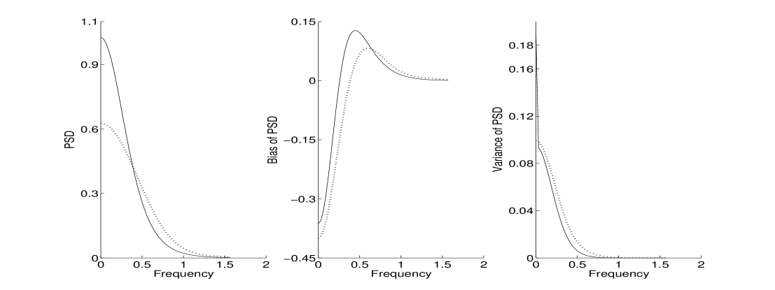
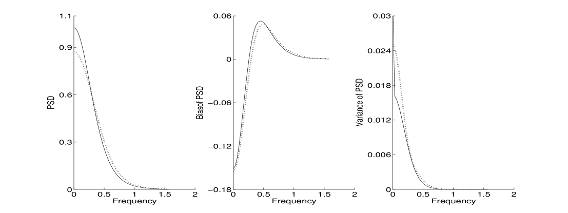
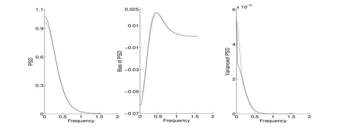
Figure 1: The average estimated power spectral density $\widehat{\phi}_{n}(\cdot)$ (left column), the bias (middle column) and the variance (right column) for sample sizes 100 (top row), 1000 (middle row) and 10000 (bottom row). The solid and the dotted lines correspond to theoretical (asymptotic) and empirical values, respectively.

From these figures, it can be observed that as the sample size goes from 100 to 10000, the empirical values of bias and variance get closer to the asymptotic results. Moreover, the theoretical (asymptotic) computations are quite comparable to the empirical values, even for sample size 100.

IV-B Finite sample comparison of $\widehat{\phi}_{n}(\lambda)$ with Poisson sampled estimator $\widehat{\psi}_{n}(\lambda)$

We generate Poisson sampled data with the average sampling rate $\rho=1$ for sample sizes $n=100$, 1000 and 10000, and compute the estimator $\widehat{\psi}_{n}(\lambda)$ on $[0,\pi/2]$. Here, the optimal power of $n$ for the window width is $b_{n}\propto n^{-1/5}$. We use $b_{n}=\frac{1}{4}n^{-1/5}$.

Figure 2 shows the empirical bias, variance and MSE of the estimators $\widehat{\phi}_{n}(\lambda)$ and $\widehat{\psi}_{n}(\lambda)$ computed from 500 simulation runs, as a function of the frequency, for sample sizes 100, 1000 and 10000.

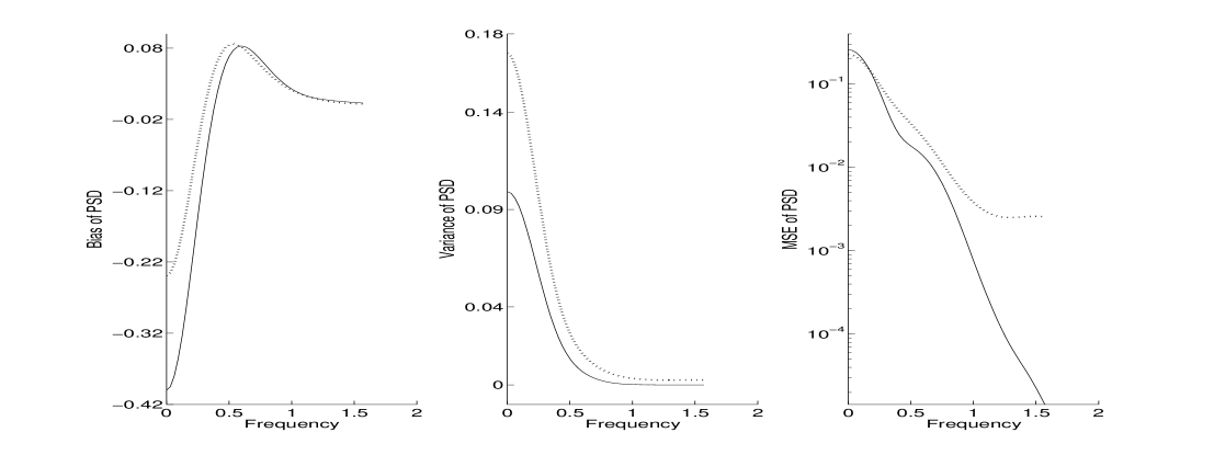
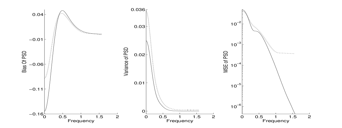
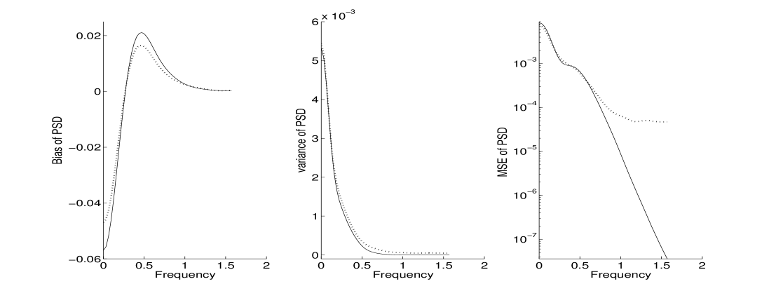
Figure 2: The estimated bias of the power spectral density $\widehat{\phi}_{n}(\cdot)$ and $\widehat{\psi}_{n}(\cdot)$ (left column), the variance (middle column) and the MSE (in log scale, right column) for sample sizes 100 (top row), 1000 (middle row) and 10000 (bottom row). The solid and the dotted lines correspond to regular and Poisson samplings, respectively.

From these figures, it can be observed that the bias of $\widehat{\psi}_{n}(\cdot)$ is generally less than that of $\widehat{\phi}_{n}(\cdot)$ while the variance of $\widehat{\psi}_{n}(\cdot)$ is larger than that of $\widehat{\phi}_{n}(\cdot)$. The differences diminish with larger sample size. These patterns are in accordance with the large sample comparisons made in Section III-B. The MSE of $\widehat{\psi}_{n}(\cdot)$ is larger than that of the $\widehat{\phi}_{n}(\cdot)$ for larger frequencies. The MSE is plotted in log-scale in order to highlight the fact that this quantity, in the case of $\widehat{\psi}_{n}(\cdot)$, levels off to a constant value for larger frequencies, while in the case of $\widehat{\phi}_{n}(\cdot)$, it continues to decline. This difference in behaviour is in accordance with the variance expressions given in (III.4) and (III.10).

V Discussion

In this paper, we have shown that the smoothed periodogram based on regularly spaced samples of a continuous time stationary stochastic process is consistent, under certain conditions, provided that the sampling rate increases appropriately as the sample size goes to infinity. We have also shown that, under the conditions used in the proofs, the estimators based on uniformly and non-uniformly spaced samples have about the same rates of convergence. Thus, our results remove a widely perceived theoretical deficiency of a popular spectral estimator based on regular sampling.

It has been a common experience, both theoretically and empirically[22], that the smoothed periodogram estimator (I.1) of a non-bandlimited power spectral density has less variance and more bias compared to the corresponding estimator $\widehat{\psi}_{n}(\cdot)$ based on Poisson sampling. What the results of Section III show is that, even though the new asymptotic results presented in this paper establish consistency of the smoothed periodogram $\widehat{\phi}_{n}(\cdot)$ and the rates of convergence of the estimators $\widehat{\phi}_{n}(\cdot)$ and $\widehat{\psi}_{n}(\cdot)$ are comparable, the constants for the first order approximations of the bias and variance of the two estimators exhibit the same type of trade off, i.e., the constant for the bias term is larger in the case of $\widehat{\phi}_{n}(\cdot)$, and the constant for the variance term is larger in the case of $\widehat{\psi}_{n}(\cdot)$.

The new asymptotic calculations provide a theoretical justification of using the smoothed periodogram with common sense, even if the underlying power spectral density is not bandlimited. This common sense approach consists of appropriate filtering of the continuous time process followed by sampling at a suitably uniform rate. Remark 6 and Theorem 4 give guidelines for choosing a suitable filter and an appropriate sampling rate, respectively, which may be useful for practitioners.

The simulation results reported in Section IV illustrate how one can choose an appropriate sampling rate for estimating the power spectral density, and obtain results in line with the theoretical results. Even though the underlying spectral density in this example is not band-limited, the estimator $\widehat{\phi}_{n}(\cdot)$ (based on uniformly spaced samples) is found to have smaller MSE than $\widehat{\psi}_{n}(\cdot)$ (based on Poisson samples) for larger frequencies. The reverse order holds for smaller frequencies. This shows that there is no clear dominance of one kind of sampling over another. This finding for finite samples complements our asymptotic results.

Our results do not take anything away from the vast literature on spectrum estimation through irregularly sampled data. These methods may be quite appropriate when one does not have control over the sampling mechanism, when irregular sampling is logistically feasible and methodologically not limited, or when regular sampling have to be avoided for a specific reason (other than its perceived inconsistency). Further, an irregular sampling scheme such as Poisson sampling can be used where an estimator based on it is expected, either through theoretical analysis or through simulation studies, to have smaller MSE than the corresponding estimator based on regular sampling scheme.

We have shown in Section III-B how our theoretical results can be used to compare uniform and Poisson sampling schemes. The results compiled there may be used to make further comparisons under different constraints. For example, if there is a limit to the maximum average sampling rate and/or the maximum sample size, one may make an optimal choice of the window width for fixed values of these two parameters, and then determine the corresponding MSE. In the case of $\widehat{\phi}_{n}(\cdot)$, the optimal choice of the window width (for given sample size and sampling rate) is given by (A.19), while the choice in the case of $\widehat{\psi}_{n}(\cdot)$ can be derived similarly from (III.6) and (III.7)[6]. The best rates and constants achievable under the two sampling schemes, under appropriate constraints, may then be used to make a suitable choice of the sampling scheme. However, if there is a hard restriction on the minimum separation between two successive samples (rather than a restriction on the average sampling rate), then one cannot use Poisson sampling at all. In such cases, irregular sampling may be done according to a renewal process, with the inter-sample distance having a restricted probability distribution. Such a sampling scheme would not satisfy the sufficient condition for alias-free sampling given in Theorem 1 of [5]. Thus, one may have to look further in search of a suitable estimator based on non-uniform sampling under such a restriction.

The proven consistency of the smoothed periodogram opens up the possibility of establishing consistency of parametric estimators of the power spectral density of a continuous time process based on regularly spaced samples, by allowing the sampling rate together with the sample size to go to infinity. Such asymptotic calculations may potentially be used to justify and/or fine-tune multi-resolution methods of spectrum estimation[21].

We denote by $K_{1}(\cdot)$ a function that bounds the covariance averaging kernel $K(\cdot)$ as in Condition 2. Further, we denote $K_{1}(0)$ by $M$.

Proof of Theorem 1.  We shall show that the bias of the estimator $\widehat{\phi}_{n}(\lambda)$ given by (I.2) converges to $0$ uniformly over $[\lambda_{l},\lambda_{u}]$ for any $\lambda_{l}$, $\lambda_{u}$ such that $\lambda_{l}<\lambda_{u}$. In order to compute the bias, we evaluate $E[\widehat{\gamma}_{n}(v)]$:

$$E[\widehat{\gamma}_{n}(v)] =E\left[\frac{1}{n}\sum_{j=1}^{n-|v|}X\left(\frac{j}{\rho_{n}}\right)X\left(\frac{j+|v|}{\rho_{n}}\right)\right]$$

$$=\left(1-\frac{|v|}{n}\right)C\left(\frac{v}{\rho_{n}}\right).$$ (A.1)

Therefore, we have

$$\hskip-7.0ptE[\widehat{\phi}_{n}(\lambda)]$$

$$= \frac{1}{2\pi\rho_{n}}\sum_{|v|<n}\!\left(1\!-\!\frac{|v|}{n}\right)C\left(\frac{v}{\rho_{n}}\right)K(b_{n}v)e^{\frac{-iv\lambda}{\rho_{n}}}1_{[-\pi\rho_{n},\pi\rho_{n}]}(\lambda).$$

Consider the simple function $S_{n}(\cdot)$, defined over $[\lambda_{l},\lambda_{u}]\times(-\infty,\infty)$, by

$$S_{n}(\lambda,t)= \frac{1}{2\pi}\sum_{|v|<n}\left(1-\frac{|v|}{n}\right)C\left(\frac{v}{\rho_{n}}\right)K\left(b_{n}v\right)e^{\frac{-iv\lambda}{\rho_{n}}}$$

$$\times 1_{[-\pi\rho_{n},\pi\rho_{n}]}(\lambda)1_{\left(\frac{v-1}{\rho_{n}},\frac{v}{\rho_{n}}\right]}(t).$$

Observe that $\int_{-\infty}^{\infty}S_{n}(\lambda,t)dt=E[\widehat{\phi}_{n}(\lambda)]$.
Define the function $S(\cdot)$, over $[\lambda_{l},\lambda_{u}]\times(-\infty,\infty)$, by

$$\hskip-80.0ptS(\lambda,t)=\frac{1}{2\pi}C(t)e^{-it\lambda}.$$

Observe that $\int_{-\infty}^{\infty}S(\lambda,t)dt=\phi(\lambda)$ which is continuous.

For any $t\in(-\infty,\infty)$, let $v_{n}(t)$ be the smallest integer greater than or equal to $\rho_{n}t$. Note that the interval $(\frac{v_{n-1}(t)}{\rho_{n}},\frac{v_{n}(t)}{\rho_{n}}]$ contains the point $t$ and $\lim_{n\rightarrow\infty}\frac{v_{n}(t)}{\rho_{n}}=t$. For sufficiently large $n$, we have from Conditions 3 and 4,

$$S_{n}(\lambda,t)= \frac{1}{2\pi}\left(1-\frac{|v_{n}(t)|}{\rho_{n}}\cdot\frac{\rho_{n}}{n}\right)C\left(\frac{v_{n}(t)}{\rho_{n}}\right)K\left(b_{n}\rho_{n}\frac{v_{n}(t)}{\rho_{n}}\right)$$

$$\times e^{\frac{-iv_{n}(t)\lambda}{\rho_{n}}}1_{[-\pi\rho_{n},\pi\rho_{n}]}(\lambda).$$

Proving the uniform convergence of $Bias[\widehat{\phi}_{n}(\lambda)]$ over finite interval $[\lambda_{l},\,\lambda_{u}]$ amounts to proving

$$\lim_{n\rightarrow\infty}\int_{-\infty}^{\infty}S_{n}(\lambda,t)dt=\int_{-\infty}^{\infty}S(\lambda,t)dt,$$

uniformly over $[\lambda_{l},\,\lambda_{u}]$. By virtue of the continuity of the limiting function, this in turn is equivalent to proving that $\int_{-\infty}^{\infty}S_{n}(\lambda,t)dt$ converges continuously over this interval [27], i.e., for any sequence $\lambda_{n}\rightarrow\lambda$,

$$\lim_{n\rightarrow\infty}\int_{-\infty}^{\infty}S_{n}(\lambda_{n},t)dt=\int_{-\infty}^{\infty}S(\lambda,t)dt$$

where $\lambda_{n},\lambda\in[\lambda_{l},\,\lambda_{u}]$.

By continuity of the function $S_{n}(\lambda,t)$ with respect to $t$ and $\lambda$, we have from Conditions 3 and 4, for any fixed $t$,

$$\lim_{n\rightarrow\infty}|S_{n}(\lambda_{n},t)-S(\lambda,t)|=0.$$

Note that from Conditions 1 and 2, we have the dominance

$$|S_{n}(\lambda_{n},t)|\leq M\sum_{|v|<n}\left|C\left(\frac{v}{\rho_{n}}\right)\right|1_{\left(\frac{v-1}{\rho_{n}},\frac{v}{\rho_{n}}\right]}(t)\leq Mh_{0}(t).$$

where $h_{0}(\cdot)$ is the function described in Condition 1. Thus, by applying the dominated convergence theorem (DCT), we have

$$\lim_{n\rightarrow\infty}\int_{-\infty}^{\infty}S_{n}(\lambda_{n},t)dt=\int_{-\infty}^{\infty}S(\lambda,t)dt.$$

Hence, $E[\widehat{\phi}_{n}(\lambda)]\rightarrow\phi(\lambda)$ uniformly on $[\lambda_{l},\,\lambda_{u}]$. $\Box$

Proof of Theorem 2.  The estimator $\widehat{\phi}_{n}(\lambda)$, given by (I.2), can be written as

$$\widehat{\phi}_{n}(\lambda)=\frac{1}{2\pi\rho_{n}}\widehat{\gamma}_{n}(0)+\frac{1}{\pi\rho_{n}}\sum_{v=1}^{n-1}\widehat{\gamma}_{n}(v)K(b_{n}v)\cos\left(\frac{\lambda v}{\rho_{n}}\right).$$

Therefore,

$$Var[\widehat{\phi}_{n}(\lambda)]=I_{1}+2I_{2}(\lambda)+I_{3}(\lambda),$$ (A.2)

where

$$I_{1} = \frac{1}{(2\pi)^{2}\rho_{n}^{2}}Var[\widehat{\gamma}_{n}(0)],$$

$$I_{2}(\lambda) = Cov\left[\frac{1}{2\pi\rho_{n}}\widehat{\gamma}_{n}(0),\frac{1}{\pi\rho_{n}}\sum_{v=1}^{n-1}\widehat{\gamma}_{n}(v)K(b_{n}v)\cos\!\left(\frac{\lambda v}{\rho_{n}}\right)\!\right]\!,$$

$$I_{3}(\lambda) = Var\left[\frac{1}{\pi\rho_{n}}\sum_{v=1}^{n-1}\widehat{\gamma}_{n}(v)K(b_{n}v)\cos\left(\frac{\lambda v}{\rho_{n}}\right)\right]\!.$$

Before we consider the convergence of the above three terms, we simplify the computation of $Cov(\widehat{\gamma}_{n}(v_{1}),\widehat{\gamma}_{n}(v_{2}))$ for non negative $v_{1}$ and $v_{2}$. Note from Condition 5 that

$$\begin{split}&\hskip-7.0ptE[\widehat{\gamma}_{n}(v_{1})\widehat{\gamma}_{n}(v_{2})]\\ =&E\left[\frac{1}{n^{2}}\sum_{j=1}^{n-v_{1}}\sum_{l=1}^{n-v_{2}}X\!\!\left(\frac{j}{\rho_{n}}\right)X\!\!\left(\frac{j\!+\!v_{1}}{\rho_{n}}\right)X\!\!\left(\frac{l}{\rho_{n}}\right)X\!\!\left(\frac{l\!+\!v_{2}}{\rho_{n}}\right)\right]\\ =&\frac{1}{n^{2}}\sum_{j=1}^{n-v_{1}}\sum_{l=1}^{n-v_{2}}\left[C\!\!\left(\frac{v_{1}}{\rho_{n}}\!\right)\!C\!\!\left(\frac{v_{2}}{\rho_{n}}\!\right)+C\!\!\left(\!\frac{j\!-\!l\!+\!v_{1}}{\rho_{n}}\!\right)\!C\!\!\left(\!\frac{j\!-\!l\!-\!v_{2}}{\rho_{n}}\!\right)\right.\\ &\left.~{}+C\!\!\left(\!\frac{j\!-\!l}{\rho_{n}}\right)\!C\!\!\left(\!\frac{j\!-\!l\!+\!v_{1}\!-\!v_{2}}{\rho_{n}}\right)+Q\!\!\left(\frac{v_{1}}{\rho_{n}},\frac{l\!-\!j}{\rho_{n}},\frac{l\!-\!j\!+\!v_{2}}{\rho_{n}}\right)\right]\\ =&\left(1-\frac{v_{1}}{n}\right)C\!\!\left(\frac{v_{1}}{\rho_{n}}\right)\left(1-\frac{v_{2}}{n}\right)C\!\!\left(\frac{v_{2}}{\rho_{n}}\right)\\ &~{}+\frac{1}{n}\sum_{|u|<n}U_{n}(u,v_{1},v_{2})~{}C\!\!\left(\frac{u+v_{1}}{\rho_{n}}\right)C\!\!\left(\frac{u-v_{2}}{\rho_{n}}\right)\\ &~{}+\frac{1}{n}\sum_{|u|<n}U_{n}(u,v_{1},v_{2})~{}C\!\!\left(\frac{u}{\rho_{n}}\right)C\!\!\left(\frac{u+v_{1}-v_{2}}{\rho_{n}}\right)\\ &~{}+\frac{1}{n}\sum_{|u|<n}U_{n}(u,v_{1},v_{2})~{}Q\!\!\left(\frac{v_{1}}{\rho_{n}},\frac{-u}{\rho_{n}},\frac{-u+v_{2}}{\rho_{n}}\right),\end{split}$$ (A.3)

where $U_{n}(u,v_{1},v_{2})$ is a function with values between 0 and 1 defined as follows

$$\begin{split}&\hskip-7.0ptU_{n}(u,v_{1},v_{2})\\ =&\begin{cases}0,&u\leq-n+v_{2},\\ 1-\frac{v_{2}\!-\!u}{n}&-n\!+\!v_{2}\!<\!u\!<\!\min(0,v_{2}\!-\!v_{1}),\\ 1-\frac{\max(v_{1},v_{2})}{n}&\min(0,v_{2}\!-\!v_{1})\leq u\leq\max(0,v_{2}\!-\!v_{1}),\\ 1-\frac{u\!+\!v_{1}}{n}&\max(0,v_{2}\!-\!v_{1})<u<n\!-\!v_{1},\\ 0&u\geq n\!-\!v_{1}.\end{cases}\end{split}$$ (A.4)

Therefore, by using (A.1) and (A.3), we have

$$\begin{split}&\hskip-10.0ptCov(\widehat{\gamma}_{n}(v_{1}),\widehat{\gamma}_{n}(v_{2}))\\ =&E[\widehat{\gamma}_{n}(v_{1})\widehat{\gamma}_{n}(v_{2})]-E[\widehat{\gamma}_{n}(v_{1})]E[\widehat{\gamma}_{n}(v_{2})]\\ =&\frac{1}{n}\sum_{|u|<n}U_{n}(u,v_{1},v_{2})C\left(\frac{u+v_{1}}{\rho_{n}}\right)C\left(\frac{u-v_{2}}{\rho_{n}}\right)\\ &+\frac{1}{n}\sum_{|u|<n}U_{n}(u,v_{1},v_{2})C\left(\frac{u}{\rho_{n}}\right)C\left(\frac{u+v_{1}-v_{2}}{\rho_{n}}\right)\\ &+\frac{1}{n}\sum_{|u|<n}U_{n}(u,v_{1},v_{2})Q\left(\frac{v_{1}}{\rho_{n}},\frac{-u}{\rho_{n}},\frac{-u+v_{2}}{\rho_{n}}\right).\end{split}$$ (A.5)

We now use this simplified form of $Cov(\widehat{\gamma}_{n}(v_{1}),\widehat{\gamma}_{n}(v_{2}))$ to establish the convergence of the three terms, $I_{1}$, $I_{2}(\lambda)$ and $I_{3}(\lambda)$.

Using (A.5) and Condition 5, $I_{1}$ is given as

$$I_{1}= \frac{1}{(2\pi)^{2}\rho_{n}^{2}}\left[\frac{2}{n}\sum_{|u|<n}U_{n}(u,0,0)C\left(\frac{u}{\rho_{n}}\right)^{2}\right.$$

$$\left.+\frac{1}{n}\sum_{|u|<n}U_{n}(u,0,0)Q\left(0,\frac{-u}{\rho_{n}},\frac{-u}{\rho_{n}}\right)\right]$$

$$\leq \frac{2C(0)}{(2\pi)^{2}n\rho_{n}}\sum_{|u|<n}\!\left|C\!\!\left(\frac{u}{\rho_{n}}\!\right)\!\right|\frac{1}{\rho_{n}}+\frac{g_{1}(0)g_{2}(0)}{(2\pi)^{2}n\rho_{n}}\!\sum_{|u|<n}\!\!g_{3}\!\!\left(\frac{u}{\rho_{n}}\!\right)\!\!\frac{1}{\rho_{n}}.$$

As in Theorem 1, we can view $\sum_{|u|<n}\!\left|C\!\!\left(\frac{u}{\rho_{n}}\!\right)\!\right|\frac{1}{\rho_{n}}$ as the integral of the function $s_{n}(\cdot)$ defined by

$$s_{n}(t)=\sum_{|i|<n}\left|C\left(\frac{i}{\rho_{n}}\right)\right|1_{(\frac{i-1}{\rho_{n}},\frac{i}{\rho_{n}}]}(t).$$

Since $s_{n}(t)\!\rightarrow\!|C(t)|$, and $s_{n}(t)\!\leq\!h_{0}(t)$ holds from Condition 1, we get $\lim_{n\rightarrow\infty}\sum_{|u|<n}\left|C\!\!\left(\frac{u}{\rho_{n}}\right)\right|\frac{1}{\rho_{n}}\!=\!\int_{-\infty}^{\infty}|C(t)|dt$ by applying the DCT as in Theorem 1, under Condition 4. A similar argument, together with Conditions 4 and 5, ensures that $\lim_{n\rightarrow\infty}\sum_{|u|<n}g_{3}\left(\frac{u}{\rho_{n}}\right)\frac{1}{\rho_{n}}=\int_{-\infty}^{\infty}|g_{3}(u)|du$. Both the limiting integrals are finite. So $nb_{n}I_{1}\rightarrow 0$ as $n\rightarrow\infty$.

Using (A.5) and Condition 5, the term $I_{2}(\lambda)$ is given as

$$\begin{split}&\hskip-10.0pt|I_{2}(\lambda)|\\ \hskip-3.0pt\leq&\frac{1}{2\pi^{2}\rho_{n}^{2}}\sum_{v=1}^{n-1}\left|\frac{1}{n}\sum_{|u|<n}\!U_{n}(u,0,v)~{}C\!\!\left(\frac{u}{\rho_{n}}\right)C\!\!\left(\frac{u\!+\!v}{\rho_{n}}\right)\!\right||K(b_{n}v)|\\ +&\frac{1}{2\pi^{2}\rho_{n}^{2}}\sum_{v=1}^{n-1}\left|\frac{1}{n}\sum_{|u|<n}\!U_{n}(u,0,v)~{}C\!\!\left(\frac{u}{\rho_{n}}\right)C\!\!\left(\frac{u\!-\!v}{\rho_{n}}\right)\!\right||K(b_{n}v)|\\ +&\frac{1}{2\pi^{2}\rho_{n}^{2}}\sum_{v=1}^{n-1}\left|\frac{1}{n}\sum_{|u|<n}\!U_{n}(u,0,v)~{}Q\!\!\left(\frac{v}{\rho_{n}},\frac{-u}{\rho_{n}},\frac{-u}{\rho_{n}}\right)\!\right||K(b_{n}v)|\\ \hskip-3.0pt\leq&\frac{|C(0)|}{\pi^{2}nb_{n}\rho_{n}}\left(\sum_{|u|<n}\left|C\!\!\left(\frac{u}{\rho_{n}}\right)\right|\frac{1}{\rho_{n}}\right)\left(\sum_{v=1}^{n-1}|K(b_{n}v)|b_{n}\right)\\ &+\frac{|g_{1}(0)g_{2}(0)|}{2\pi^{2}nb_{n}\rho_{n}}\left(\sum_{|u|<n}g_{3}\!\!\left(\frac{u}{\rho_{n}}\right)\frac{1}{\rho_{n}}\right)\left(\sum_{v=1}^{n-1}|K(b_{n}v)|b_{n}\right).\end{split}$$

The last expression does not depend on $\lambda$. An argument as in the case of $I_{1}$ will show that $\lim_{n\rightarrow\infty}\sum_{v=1}^{n-1}|K(b_{n}v)|b_{n}=\int_{0}^{\infty}K(x)dx$, under Conditions 2 and 3. The convergence of the other sums have already been discussed in connection with the term $I_{1}$. Hence, $nb_{n}I_{2}(\lambda)\rightarrow 0$ as $n\rightarrow\infty$ uniformly for all $\lambda$.

Now we will consider $I_{3}(\lambda)$. Using (A.5), this term can be written as

$$\begin{split}I_{3}(\lambda)=&\frac{1}{\pi^{2}\rho_{n}^{2}}\sum_{v_{1}=1}^{n-1}\sum_{v_{2}=1}^{n-1}Cov[\widehat{\gamma}_{n}(v_{1}),\widehat{\gamma}_{n}(v_{2})]K(b_{n}v_{1})K(b_{n}v_{2})\\ &\times\cos\left(\frac{\lambda v_{1}}{\rho_{n}}\right)\cos\left(\frac{\lambda v_{2}}{\rho_{n}}\right)\\ =&I_{31}(\lambda)+I_{32}(\lambda)+I_{33}(\lambda),\end{split}$$

where

$$\begin{split}I_{31}(\lambda)=&\frac{1}{\pi^{2}\rho_{n}^{2}}\sum_{v_{1}=1}^{n-1}\sum_{v_{2}=1}^{n-1}K(b_{n}v_{1})K(b_{n}v_{2})\cos\!\left(\!\frac{\lambda v_{1}}{\rho_{n}}\!\!\right)\cos\!\left(\!\frac{\lambda v_{2}}{\rho_{n}}\!\!\right)\\ &\times\frac{1}{n}\sum_{u=-(n-1)}^{(n-1)}U_{n}(u,v_{1},v_{2})~{}C\!\left(\!\frac{u+v_{1}}{\rho_{n}}\!\right)C\!\left(\!\frac{u-v_{2}}{\rho_{n}}\!\right)\!,\end{split}$$

$$\begin{split}I_{32}(\lambda)=&\frac{1}{\pi^{2}\rho_{n}^{2}}\sum_{v_{1}=1}^{n-1}\sum_{v_{2}=1}^{n-1}K(b_{n}v_{1})K(b_{n}v_{2})\cos\!\left(\!\frac{\lambda v_{1}}{\rho_{n}}\!\!\right)\cos\!\left(\!\frac{\lambda v_{2}}{\rho_{n}}\!\!\right)\\ &\times\frac{1}{n}\sum_{u=-(n-1)}^{(n-1)}\!\!U_{n}(u,v_{1},v_{2})~{}C\!\left(\!\frac{u}{\rho_{n}}\!\right)C\!\left(\!\frac{u+v_{1}-v_{2}}{\rho_{n}}\!\right)\!,\end{split}$$

and

$$\begin{split}&\hskip-15.0ptI_{33}(\lambda)\\ =&\frac{1}{\pi^{2}\rho_{n}^{2}}\sum_{v_{1}=1}^{n-1}\sum_{v_{2}=1}^{n-1}\!K(b_{n}v_{1})K(b_{n}v_{2})\cos\!\left(\!\frac{\lambda v_{1}}{\rho_{n}}\!\right)\cos\!\left(\!\frac{\lambda v_{2}}{\rho_{n}}\!\right)\!\\ &\times\frac{1}{n}\sum_{u=-(n-1)}^{(n-1)}U_{n}(u,v_{1},v_{2})~{}Q\!\left(\!\frac{v_{1}}{\rho_{n}},\frac{-u}{\rho_{n}},\frac{-u+v_{2}}{\rho_{n}}\!\!\right).\end{split}$$

From Conditions 2 and 5,

$$\hskip-7.0pt|nb_{n}I_{33}(\lambda)|$$

$$\leq M^{2}\rho_{n}b_{n}\frac{1}{\rho_{n}^{3}}\!\sum_{v_{1}=1}^{n-1}\sum_{v_{2}=1}^{n-1}\sum_{u=-(n-1)}^{(n-1)}\!\!g_{1}\!\!\left(\frac{v_{1}}{\rho_{n}}\!\right)g_{2}\!\!\left(\frac{u}{\rho_{n}}\!\right)g_{3}\!\!\left(\!\frac{u\!+\!v_{2}}{\rho_{n}}\!\right)\!.$$

By using a similar argument as in the case of $I_{1}$, we have

$$\hskip-5.0pt\lim_{n\rightarrow\infty}\frac{1}{\rho_{n}^{3}}\!\sum_{v_{1}=1}^{n-1}\sum_{v_{2}=1}^{n-1}\sum_{u=-(n-1)}^{(n-1)}\!g_{1}\!\left(\frac{v_{1}}{\rho_{n}}\right)\!g_{2}\!\left(\frac{u}{\rho_{n}}\right)\!g_{3}\!\left(\!\frac{u\!+\!v_{2}}{\rho_{n}}\!\!\right)$$

$$=\int_{0}^{\infty}g_{1}(v_{1})dv_{1}\int_{0}^{\infty}\left[\int_{-\infty}^{\infty}g_{2}(u)g_{3}(u+v_{2})du\right]dv_{2}.$$

Hence, $nb_{n}I_{33}(\lambda)\rightarrow 0$ as $n\rightarrow\infty$ uniformly for all $\lambda$.

Consider the term $I_{31}(\lambda)$, let $j\!=\!v_{1}+v_{2},~{}l\!=\!u-v_{2},~{}i\!=\!v_{2}$.

$$\hskip-8.0ptI_{31}(\lambda)$$

$$= \frac{1}{\pi^{2}\rho_{n}^{2}}\sum_{i=1}^{n-1}\sum_{j=i+1}^{n-1+i}\!K(b_{n}i)K(b_{n}(j\!-\!i))\cos\!\!\left(\frac{\lambda i}{\rho_{n}}\!\right)\cos\!\!\left(\!\frac{\lambda(j\!-\!i)}{\rho_{n}}\!\right)$$

$$\times\frac{1}{n}\sum_{l=-(n-1)-i}^{(n-1)-i}U_{n}(l+i,j-i,i)~{}C\!\!\left(\frac{j+l}{\rho_{n}}\right)C\!\!\left(\frac{l}{\rho_{n}}\right).$$

From Condition 2, observe that

$$\hskip-7.0ptnb_{n}|I_{31}(\lambda)|$$

$$\leq M\frac{b_{n}}{\rho_{n}^{2}}\sum_{i=1}^{n-1}\sum_{j=i+1}^{n-1+i}\sum_{l=-(n-1)-i}^{(n-1)-i}\left|K(b_{n}i)~{}C\!\!\left(\!\frac{j\!+\!l}{\rho_{n}}\!\right)C\!\!\left(\!\frac{l}{\rho_{n}}\!\right)\right|.$$

Consider the simple function $S_{n}$, defined over $(0,\infty)\times(0,\infty)\times(-\infty,\infty)$ by

$$\hskip-7.0ptS_{n}(x,t,t^{{}^{\prime}})$$

$$= M\frac{1}{\pi^{2}}\sum_{i=1}^{n-1}\sum_{j=i+1}^{n-1+i}\sum_{l=-(n-1)-i}^{(n-1)-i}\left|K(b_{n}i)~{}C\!\!\left(\!\frac{j\!+\!l}{\rho_{n}}\!\right)\!C\!\!\left(\!\frac{l}{\rho_{n}}\!\right)\right|$$

$$\times\!1_{((i-1)b_{n},ib_{n}]}(x)1_{(\frac{j-1}{\rho_{n}},\frac{j}{\rho_{n}}]}(t)1_{(\frac{l-1}{\rho_{n}},\frac{l}{\rho_{n}}]}(t^{{}^{\prime}}\!),$$

so that

$$nb_{n}|I_{31}(\lambda)|\leq\int_{0}^{\infty}\int_{0}^{\infty}\int_{-\infty}^{\infty}S_{n}(x,t,t^{{}^{\prime}})dxdtdt^{{}^{\prime}}.$$

Since $\lim_{n\rightarrow\infty}\rho_{n}b_{n}=0$, we have, for any fixed $(x,t,t^{\prime})\in(0,\infty)\times(0,\infty)\times(-\infty,\infty)$ and for large enough $n$, the inequality $\rho_{n}b_{n}<x/t$, i.e., $t\rho_{n}<x/b_{n}$. Therefore, for large $n$, the unique integer $j$ for which $1_{(\frac{j-1}{\rho_{n}},\frac{j}{\rho_{n}}]}(t)$ is non-zero is smaller than the unique integer $i$ for which $1_{((i-1)b_{n},ib_{n}]}(x)$ is non-zero. However, the ranges of summations in the definition of $S_{n}(x,t,t^{{}^{\prime}})$ do not permit the order $j\leq i$. Therefore, $\lim_{n\rightarrow\infty}S_{n}(x,t,t^{{}^{\prime}})=0$. From Condition 1 and 2, we have the dominance

$$|S_{n}(x,t,t^{{}^{\prime}})|\leq M|K_{1}(x)h_{0}(t+t^{{}^{\prime}})h_{0}(t^{{}^{\prime}})|\in L^{1}$$

By applying the DCT, we have

$$\lim_{n\rightarrow\infty}\int_{0}^{\infty}\int_{0}^{\infty}\int_{-\infty}^{\infty}S_{n}(x,t,t^{{}^{\prime}})dxdtdt^{{}^{\prime}}=0.$$

Since the function $S_{n}(x,t,t^{{}^{\prime}})$ does not depend on $\lambda$, we have $nb_{n}I_{31}(\lambda)\rightarrow 0$ uniformly for all $\lambda$.

In view of the convergence of the terms $I_{1}$, $I_{2}(\lambda)$, $I_{33}(\lambda)$ and $I_{31}(\lambda)$, we have

$$\lim_{n\rightarrow\infty}nb_{n}\left[Var\left(\widehat{\phi}_{n}(\lambda)\right)-I_{32}(\lambda)\right]=0$$ (A.6)

uniformly for all $\lambda$, and so we need to prove the convergence of $nb_{n}I_{32}(\lambda)$ only.

Now consider $I_{32}(\lambda)$ and let $j=v_{1}-v_{2},~{}i=v_{2},~{}l=u$.

$$\begin{split}&\hskip-7.0ptI_{32}(\lambda)\\ =&\frac{1}{\pi^{2}\rho_{n}^{2}}\sum_{i=1}^{n-1}\sum_{j=-i+1}^{n-1-i}\!\!K(b_{n}i)K(b_{n}(i\!+\!j))\cos\!\!\left(\frac{\lambda i}{\rho_{n}}\right)\cos\!\!\left(\!\frac{\lambda(i\!+\!j)}{\rho_{n}}\!\right)\\ &\times\frac{1}{n}\sum_{l=-(n-1)}^{(n-1)}U_{n}(l,i+j,i)~{}C\!\!\left(\frac{l}{\rho_{n}}\right)C\!\!\left(\frac{l+j}{\rho_{n}}\right).\end{split}$$ (A.7)

For $\lambda=0$, it follows from (A.6) and Lemma 1 below that

$$\lim_{n\rightarrow\infty}nb_{n}Var[\widehat{\phi}_{n}(0)]=2[\phi(0)]^{2}\int_{-\infty}^{\infty}K^{2}(x)dx$$ (A.8)

For $\lambda\neq 0$, we will further decompose $I_{32}(\lambda)$ as follows. By applying the formula $2\cos(a)\cos(b)=\cos(a-b)+\cos(a+b)$ and $\cos(a+b)=\cos(a)\cos(b)-\sin(a)\sin(b)$, we have

$$I_{32}(\lambda)=I_{321}(\lambda)+I_{322}(\lambda)-I_{323}(\lambda),$$

where

$$\begin{split}I_{321}(\lambda)=&\frac{1}{2\pi^{2}}\frac{1}{n\rho_{n}^{2}}\sum_{i=1}^{n-1}\sum_{j=-i+1}^{n-1-i}\!\!K(b_{n}i)K(b_{n}(i\!+\!j))\cos\!\!\left(\frac{\lambda j}{\rho_{n}}\right)\\ &\times\sum_{l=-(n-1)}^{(n-1)}U_{n}(l,i+j,i)~{}C\!\!\left(\frac{l}{\rho_{n}}\right)C\!\!\left(\frac{l+j}{\rho_{n}}\right),\end{split}$$ (A.9)

$$\begin{split}&\hskip-7.0ptI_{322}(\lambda)\\ =&\frac{1}{2\pi^{2}}\frac{1}{n\rho_{n}^{2}}\sum_{i=1}^{n-1}\sum_{j=-i+1}^{n-1-i}\!\!K(b_{n}i)K(b_{n}(i\!+\!j))\cos\!\!\left(\frac{\lambda j}{\rho_{n}}\right)\cos\!\!\left(\frac{2\lambda i}{\rho_{n}}\right)\\ &\times\sum_{l=-(n-1)}^{(n-1)}U_{n}(l,i+j,i)~{}C\!\!\left(\frac{l}{\rho_{n}}\right)C\!\!\left(\frac{l+j}{\rho_{n}}\right),\end{split}$$ (A.10)

and

$$\begin{split}&\hskip-7.0ptI_{323}(\lambda)\\ =&\frac{1}{2\pi^{2}}\frac{1}{n\rho_{n}^{2}}\sum_{i=1}^{n-1}\sum_{j=-i+1}^{n-1-i}K(b_{n}i)K(b_{n}(i\!+\!j))\sin\!\!\left(\frac{\lambda j}{\rho_{n}}\right)\sin\!\!\left(\frac{2\lambda i}{\rho_{n}}\right)\\ &\times\sum_{l=-(n-1)}^{(n-1)}U_{n}(l,i+j,i)~{}C\!\!\left(\frac{l}{\rho_{n}}\right)C\!\!\left(\frac{l+j}{\rho_{n}}\right).\end{split}$$ (A.11)

It follows from equation (A.6), Lemma 2 and Lemma 3 below that

$$\begin{split}\lim_{n\rightarrow\infty}nb_{n}Var[\widehat{\phi}_{n}(\lambda)]=&\lim_{n\rightarrow\infty}nb_{n}I_{321}(\lambda)\\ =&[\phi(\lambda)]^{2}\int_{-\infty}^{\infty}K^{2}(x)dx,\end{split}$$ (A.12)

and the convergence is uniform over any closed interval that does not include the frequency 0. This completes the proof.
$\Box$

Lemma 1.

$$\begin{split}&\hskip-25.0pt\lim_{n\rightarrow\infty}nb_{n}I_{32}(0)\\ =&\frac{1}{\pi^{2}}\int_{0}^{\infty}\!\!K^{2}(x)\int_{-\infty}^{\infty}\left[\int_{-\infty}^{\infty}C(t+t^{{}^{\prime}})C(t^{{}^{\prime}})~{}dt^{{}^{\prime}}\right]dt~{}dx.\end{split}$$

Proof of Lemma 1.  Consider the simple function $S_{n}(\cdot)$, defined over $(0,\infty)\times(-\infty,\infty)\times(-\infty,\infty)$ by

$$\hskip-7.0ptS_{n}(x,t,t^{{}^{\prime}})$$

$$= \frac{1}{\pi^{2}}\sum_{i=1}^{n-1}\sum_{j=-i+1}^{n-1-i}\sum_{l=-(n-1)}^{(n-1)}\!\!\!K(b_{n}i)K(b_{n}(i\!+\!j))U_{n}(l,i\!+\!j,i)$$

$$\times\!C\!\!\left(\!\frac{l}{\rho_{n}}\!\right)\!C\!\!\left(\!\frac{l\!+\!j}{\rho_{n}}\!\right)\!1_{((i-1)b_{n},ib_{n}]}(x)1_{(\frac{j-1}{\rho_{n}},\frac{j}{\rho_{n}}]}(t)1_{(\frac{l-1}{\rho_{n}},\frac{l}{\rho_{n}}]}(t^{{}^{\prime}}\!).$$

Observe from (A.7) that

$$nb_{n}I_{32}(0)=\int_{0}^{\infty}\int_{-\infty}^{\infty}\int_{-\infty}^{\infty}S_{n}(x,t,t^{{}^{\prime}})dxdtdt^{{}^{\prime}}.$$

Define $i_{n}(x)$, $j_{n}(t)$ and $l_{n}(t^{{}^{\prime}})$ as the smallest integers greater than or equal to $x/b_{n}$, $\rho_{n}t$ and $\rho_{n}t^{\prime}$, respectively. Thus, $(x,t,t^{{}^{\prime}})\in(b_{n}i_{n-1}(x),b_{n}i_{n}(x)]\times\left(\frac{j_{n-1}(t)}{\rho_{n}},\frac{j_{n}(t)}{\rho_{n}}\right]\times\left(\frac{l_{n-1}(t^{\prime})}{\rho_{n}},\frac{l_{n}(t^{\prime})}{\rho_{n}}\right]$ and $b_{n}i_{n}(x)\!\rightarrow\!x,\frac{j_{n}(t)}{\rho_{n}}\!\rightarrow\!t,\frac{l_{n}(t^{{}^{\prime}})}{\rho_{n}}\!\rightarrow\!t^{{}^{\prime}}$ as $n\rightarrow\infty$. Since $nb_{n}\rightarrow\infty$ and $b_{n}\rho_{n}\rightarrow 0$ as $n\rightarrow\infty$, we have, for any point $(x,t,t^{{}^{\prime}})\in(0,\infty)\times(-\infty,\infty)\times(-\infty,\infty)$ and large enough $n$, the inequalities $-\frac{x}{b_{n}\rho_{n}}<t<\frac{nb_{n}-x}{b_{n}\rho_{n}}{\displaystyle\phantom{\int}}$​​​​​, i.e., $-i_{n}(x)<j_{n}(t)<n-i_{n}(x)$. Thus, for sufficiently large $n$, we have

$$S_{n}(x,t,t^{{}^{\prime}})= \frac{1}{\pi^{2}}K(b_{n}i_{n}(x))K\left(b_{n}i_{n}(x)\!+\!b_{n}\rho_{n}\frac{j_{n}(t)}{\rho_{n}}\right)$$

$$\times\!U_{n}(l_{n}(t^{{}^{\prime}}\!),i_{n}(x)\!+\!j_{n}(t),i_{n}(x))$$

$$\times C\left(\frac{l_{n}(t^{{}^{\prime}})}{\rho_{n}}\right)C\left(\frac{l_{n}(t^{{}^{\prime}})+j_{n}(t)}{\rho_{n}}\right).$$

Also, for large $n$, we have $-(n\!-\!xb_{n})+\frac{t}{\rho_{n}}\!<\!\frac{t^{\prime}}{\rho_{n}}\!<\!(n\!-\!xb_{n})$, and so $U_{n}(l_{n}(t^{{}^{\prime}}\!),i_{n}(x)\!+\!j_{n}(t),i_{n}(x))$ is positive and it converges to 1. Therefore, by virtue of Conditions 1 and 2, we have

$$\lim_{n\rightarrow\infty}S_{n}(x,t,t^{{}^{\prime}})=\frac{1}{\pi^{2}}K^{2}(x)C(t^{{}^{\prime}})C(t^{{}^{\prime}}+t).$$

Again, from Conditions 1 and 2, we have the dominance

$$|S_{n}(x,t,t^{{}^{\prime}})|\leq M|K_{1}(x)h_{0}(t+t^{{}^{\prime}})h_{0}(t^{{}^{\prime}})|\in L^{1}.$$

By applying the DCT, we have

$$\begin{split}&\hskip-25.0pt\lim_{n\rightarrow\infty}nb_{n}I_{32}(0)\\ \!=\!&\lim_{n\rightarrow\infty}\int_{0}^{\infty}\int_{-\infty}^{\infty}\int_{-\infty}^{\infty}S_{n}(x,t,t^{{}^{\prime}})dxdtdt^{\prime}\\ \!=\!&\frac{1}{\pi^{2}}\!\int_{0}^{\infty}\!\!\!K^{2}(x)\!\int_{-\infty}^{\infty}\!\!\left[\int_{-\infty}^{\infty}\!\!\!C(t+t^{{}^{\prime}}\!)C(t^{{}^{\prime}}\!)dt^{{}^{\prime}}\!\right]\!dtdx.\end{split}$$

$\Box$

Lemma 2.

The function $I_{321}(\cdot)$ converges as follows:

$$\begin{split}&\hskip-10.0pt\lim_{n\rightarrow\infty}nb_{n}I_{321}(\lambda)\\ =&\frac{1}{2\pi^{2}}\int_{0}^{\infty}\!\!\!K^{2}(x)\int_{-\infty}^{\infty}\!\!\left[\cos(\lambda t)\!\left[\int_{-\infty}^{\infty}\!\!C(t+t^{{}^{\prime}}\!)C(t^{{}^{\prime}}\!)dt^{{}^{\prime}}\right]\!dt\right]\!dx.\end{split}$$

The convergence is uniform on $[\lambda_{l},\lambda_{u}]$ for arbitrary $\lambda_{l}$ and $\lambda_{u}$ such that $\lambda_{l}<\lambda_{u}$ and $\lambda_{l}\lambda_{u}>0$.

Proof of Lemma 2.  Consider the simple function $S_{n}(\cdot)$, defined over $[\lambda_{l},\lambda_{u}]\times(0,\infty)\times(-\infty,\infty)\times(-\infty,\infty)$ by

$$S_{n}(\lambda,x,t,t^{{}^{\prime}})= \frac{1}{2\pi^{2}}\!\sum_{i=1}^{n-1}\sum_{j=-i+1}^{n-1-i}\!\sum_{l=-(n-1)}^{(n-1)}\!\!\!K(b_{n}i)K(b_{n}(i\!+\!j))$$

$$\times\cos\!\!\left(\!\frac{\lambda j}{\rho_{n}}\!\right)U_{n}(l,i\!+\!j,i)~{}C\!\!\left(\frac{l}{\rho_{n}}\!\right)C\!\!\left(\frac{l\!+\!j}{\rho_{n}}\right)$$

$$\times 1_{((i-1)b_{n},ib_{n}]}(x)1_{(\frac{j-1}{\rho_{n}},\frac{j}{\rho_{n}}]}(t)1_{(\frac{l-1}{\rho_{n}},\frac{l}{\rho_{n}}]}(t^{{}^{\prime}}\!),$$

so that, from (A.9),

$$nb_{n}I_{321}(\lambda)=\int_{0}^{\infty}\int_{-\infty}^{\infty}\int_{-\infty}^{\infty}S_{n}(\lambda,x,t,t^{{}^{\prime}})dxdtdt^{{}^{\prime}}.$$

A similar argument as in the proof of Lemma 1 will show that for $(x,t,t^{{}^{\prime}})\in(0,\infty)\times(-\infty,\infty)\times(-\infty,\infty)$ and sufficiently large $n$,

$$S_{n}(\lambda,x,t,t^{{}^{\prime}})= \frac{1}{2\pi^{2}}K(b_{n}i_{n}(x))~{}K\!\!\left(b_{n}i_{n}(x)+b_{n}\rho_{n}\frac{j_{n}(t)}{\rho_{n}}\right)$$

$$\times\cos\!\!\left(\!\frac{\lambda j_{n}(t)}{\rho_{n}}\!\!\right)U_{n}(l_{n}(t^{{}^{\prime}}),i_{n}(x)\!+\!j_{n}(t),i_{n}(x))$$

$$\times C\!\!\left(\frac{l_{n}(t^{{}^{\prime}})}{\rho_{n}}\right)C\!\!\left(\frac{l_{n}(t^{{}^{\prime}})\!+\!j_{n}(t)}{\rho_{n}}\right),$$

where $i_{n}(x)$, $j_{n}(t)$ and $l_{n}(t^{{}^{\prime}})$ are the smallest integers greater than or equal to $x/b_{n}$, $\rho_{n}t$ and $\rho_{n}t^{\prime}$, respectively, and that the function $S_{n}(\lambda,x,t,t^{{}^{\prime}})$ converges to the function $S(\cdot)$, defined over $(0,\infty)\times(-\infty,\infty)\times(-\infty,\infty)$ by

$$S(\lambda,x,t,t^{{}^{\prime}})=\frac{1}{2\pi^{2}}K^{2}(x)\cos(\lambda t)C(t^{{}^{\prime}})C(t^{{}^{\prime}}+t).$$

Observe also that $\int_{0}^{\infty}\int_{-\infty}^{\infty}\int_{-\infty}^{\infty}S(\lambda,x,t,t^{{}^{\prime}})dxdtdt^{{}^{\prime}}$ is a continuous function in $\lambda$. As in the proof of Theorem 1, we prove the convergence of $\int_{0}^{\infty}\int_{-\infty}^{\infty}\int_{-\infty}^{\infty}S_{n}(\lambda,x,t,t^{{}^{\prime}})dxdtdt^{{}^{\prime}}$uniformly on $[\lambda_{l},\lambda_{u}]$, by showing that for any sequence $\lambda_{n}\rightarrow\lambda$,

$$\begin{split}&\hskip-40.0pt\lim_{n\rightarrow\infty}\int_{0}^{\infty}\int_{-\infty}^{\infty}\int_{-\infty}^{\infty}S_{n}(\lambda_{n},x,t,t^{{}^{\prime}})dxdtdt^{{}^{\prime}}\\ &\mbox{}\qquad=\int_{0}^{\infty}\int_{-\infty}^{\infty}\int_{-\infty}^{\infty}S(\lambda,x,t,t^{{}^{\prime}})dxdtdt^{{}^{\prime}}\end{split}$$

for $\lambda_{n},\lambda\in[\lambda_{l},\lambda_{u}]$. The latter convergence follows, through Condition 1 and 2 and the DCT, from the dominance

$$|S_{n}(\lambda,x,t,t^{{}^{\prime}})|\leq M|K_{1}(x)h_{0}(t+t^{{}^{\prime}})h_{0}(t^{{}^{\prime}})|\in L^{1},$$

and the convergence of the integrand, which holds because of the continuity of the kernel, the cosine and the covariance function.

Hence, $nb_{n}I_{321}(\cdot)$ converges as stated uniformly on $[\lambda_{l},\lambda_{u}]$.
$\Box$

Lemma 3.

The functions $nb_{n}I_{322}(\cdot)$ and $nb_{n}I_{323}(\cdot)$ converge to $0$ uniformly on $[\lambda_{l},\lambda_{u}]$ for arbitrary $\lambda_{l}$ and $\lambda_{u}$ such that $\lambda_{l}<\lambda_{u}$ and $\lambda_{l}\lambda_{u}>0$.

Proof of Lemma 3.  Consider the simple function $S_{n}(\cdot)$, defined over $[\lambda_{l},\lambda_{u}]\times(0,\infty)\times(-\infty,\infty)\times(-\infty,\infty)$ by

$$\hskip-10.0ptS_{n}(\lambda,x,t,t^{{}^{\prime}})$$

$$= \frac{1}{2\pi^{2}}\sum_{i=1}^{n-1}\sum_{j=-i+1}^{n-1+i}\sum_{l=-(n-1)}^{(n-1)}K(b_{n}i)K(b_{n}(i+j))\cos\!\left(\frac{\lambda j}{\rho_{n}}\right)$$

$$\times\cos\!\left(\frac{2\lambda b_{n}i}{\rho_{n}b_{n}}\right)U_{n}(l,i\!+\!j,i)~{}C\!\!\left(\frac{l}{\rho_{n}}\right)C\!\!\left(\frac{l+j}{\rho_{n}}\right)$$

$$\times 1_{((i-1)b_{n},ib_{n}]}(x)\times 1_{(\frac{j-1}{\rho_{n}},\frac{j}{\rho_{n}}]}(t)1_{(\frac{l-1}{\rho_{n}},\frac{l}{\rho_{n}}]}(t^{{}^{\prime}}),$$

so that, from (A.10),

$$nb_{n}I_{322}(\lambda)=\int_{0}^{\infty}\int_{-\infty}^{\infty}\int_{-\infty}^{\infty}S_{n}(\lambda,x,t,t^{{}^{\prime}})dxdtdt^{{}^{\prime}}.$$ (A.13)

A similar argument as in the proof of Lemma 1 will show that for $(x,t,t^{{}^{\prime}})\in(0,\infty)\times(-\infty,\infty)\times(-\infty,\infty)$ and sufficiently large $n$,

$$\hskip-10.0ptS_{n}(\lambda,x,t,t^{{}^{\prime}})$$

$$= \frac{1}{2\pi^{2}}K(b_{n}i_{n}(x))K\left(b_{n}i_{n}(x)+b_{n}\rho_{n}\frac{j_{n}(t)}{\rho_{n}}\right)\cos\!\left(\frac{\lambda j_{n}(t)}{\rho_{n}}\right)$$

$$\times\cos\!\left(\frac{2\lambda i_{n}(x)b_{n}}{b_{n}\rho_{n}}\right)U_{n}(l_{n}(t^{{}^{\prime}}),j_{n}(t)+i_{n}(x),i_{n}(x))$$

$$\times C\!\!\left(\frac{l_{n}(t^{{}^{\prime}})}{\rho_{n}}\right)C\!\!\left(\frac{l_{n}(t^{{}^{\prime}})+j_{n}(t)}{\rho_{n}}\right),$$

where $i_{n}(x)$, $j_{n}(t)$ and $l_{n}(t^{{}^{\prime}})$ are the smallest integers greater than or equal to $x/b_{n}$, $\rho_{n}t$ and $\rho_{n}t^{\prime}$, respectively.

For obtaining the uniform convergence of $I_{322}(\cdot)$, consider

$$\hskip-10.0pt\sup_{\lambda\in[\lambda_{l},\lambda_{u}]}\left|\int_{0}^{\infty}\!\!\int_{-\infty}^{\infty}\!\!\int_{-\infty}^{\infty}\!\!S_{n}(\lambda,x,t,t^{{}^{\prime}})dxdtdt^{{}^{\prime}}\right|$$

$$\!\leq\! \sup_{\lambda\in[\lambda_{l},\lambda_{u}]}\int_{0}^{\infty}\!\!\int_{-\infty}^{\infty}\!\!\int_{-\infty}^{\infty}\!\!|S_{n}(\lambda,x,t,t^{{}^{\prime}}\!)-g_{n}(\lambda,x,t,t^{{}^{\prime}}\!)|dxdtdt^{{}^{\prime}}$$

$$~{}+\! \sup_{\lambda\in[\lambda_{l},\lambda_{u}]}\left|\int_{0}^{\infty}\int_{-\infty}^{\infty}\int_{-\infty}^{\infty}g_{n}(\lambda,x,t,t^{{}^{\prime}})dxdtdt^{{}^{\prime}}\right|,$$ (A.14)

where the function $g_{n}(\cdot)$ is defined over $[\lambda_{l},\lambda_{u}]\times(0,\infty)\times(-\infty,\infty)\times(-\infty,\infty)$ by

$$g_{n}(\lambda,x,t,t^{{}^{\prime}})=\frac{1}{2\pi^{2}}\cos(\lambda t)\cos\left(\frac{2\lambda x}{b_{n}\rho_{n}}\right)K^{2}(x)C(t^{{}^{\prime}})C(t+t^{{}^{\prime}}).$$

We shall prove the convergence of $nb_{n}I_{322}(\cdot)$ given in (A.13) by proving the convergence of the two integrals on the right hand side of (A.14).

In order to prove the first convergence, we follow the route taken in Theorem 1, i.e., we show that for any sequence $\lambda_{n}\!\rightarrow\!\lambda$

$$\lim_{n\rightarrow\infty}\int_{0}^{\infty}\!\!\!\int_{-\infty}^{\infty}\!\!\int_{-\infty}^{\infty}\!\!|S_{n}(\lambda_{n},x,t,t^{{}^{\prime}})-g_{n}(\lambda_{n},x,t,t^{{}^{\prime}})|dxdtdt^{{}^{\prime}}=0,$$

for $\lambda,\lambda_{n}\in[\lambda_{l},\lambda_{u}]$. The above integral can be written as

$$\hskip-10.0pt\int_{0}^{\infty}\int_{-\infty}^{\infty}\int_{-\infty}^{\infty}|S_{n}(\lambda_{n},x,t,t^{{}^{\prime}})-g_{n}(\lambda_{n},x,t,t^{{}^{\prime}})|dxdtdt^{\prime}$$

$$\leq \int_{0}^{\infty}\int_{-\infty}^{\infty}\int_{-\infty}^{\infty}|S_{n}(\lambda_{n},x,t,t^{{}^{\prime}})-G_{n}(\lambda_{n},x,t,t^{{}^{\prime}})|dxdtdt^{\prime}$$

$$+\int_{0}^{\infty}\int_{-\infty}^{\infty}\int_{-\infty}^{\infty}|G_{n}(\lambda_{n},x,t,t^{{}^{\prime}})-g_{n}(\lambda_{n},x,t,t^{{}^{\prime}})|dxdtdt^{\prime},$$ (A.15)

where the function $G_{n}(\cdot)$ is defined over $[\lambda_{l},\lambda_{u}]\times(0,\infty)\times(-\infty,\infty)\times(-\infty,\infty)$ by

$$\hskip-15.0ptG_{n}(\lambda,x,t,t^{{}^{\prime}})$$

$$= \frac{1}{2\pi^{2}}\cos(\lambda t)\cos\!\left(\!\frac{2\lambda i_{n}(x)b_{n}}{b_{n}\rho_{n}}\right)K^{2}(x)C(t^{{}^{\prime}})C(t+t^{{}^{\prime}})).$$

Now observe that

$$\hskip-45.0pt|S_{n}(\lambda_{n},x,t,t^{{}^{\prime}})-G_{n}(\lambda_{n},x,t,t^{{}^{\prime}})|$$

$$\leq M\left|\cos\left(\frac{2\lambda_{n}i_{n}(x)b_{n}}{b_{n}\rho_{n}}\right)\alpha_{n}(\lambda_{n},x,t,t^{{}^{\prime}})\right|,$$

where

$$\hskip-8.0pt\alpha_{n}(\lambda_{n},x,t,t^{{}^{\prime}})$$

$$= K(b_{n}i_{n}(x))\cos\!\left(\frac{\lambda_{n}j_{n}(t)}{\rho_{n}}\right)U_{n}(l_{n}(t^{{}^{\prime}}),j_{n}(t)\!+\!i_{n}(x),i_{n}(x))$$

$$\times C\!\!\left(\frac{l_{n}(t^{{}^{\prime}})}{\rho_{n}}\right)C\!\!\left(\frac{l_{n}(t^{{}^{\prime}})+j_{n}(t)}{\rho_{n}}\right)$$

$$-\cos(\lambda_{n}t)K(x)C(t^{{}^{\prime}})C(t+t^{{}^{\prime}}).$$

Since $\alpha_{n}(\lambda_{n},x,t,t^{{}^{\prime}})\rightarrow 0$ as $n\rightarrow\infty$, we have

$$\lim_{n\rightarrow\infty}|S_{n}(\lambda_{n},x,t,t^{{}^{\prime}})-G_{n}(\lambda_{n},x,t,t^{{}^{\prime}})|=0.$$

Since from Condition 1 and 2, we have the dominance

$$\hskip-40.0pt|S_{n}(\lambda_{n},x,t,t^{{}^{\prime}})-G_{n}(\lambda_{n},x,t,t^{{}^{\prime}})|$$

$$\leq 2M|K_{1}(x)h_{0}(t^{\prime})h_{0}(t+t^{\prime})|\in L^{1}.$$

By applying DCT, we have

$$\lim_{n\rightarrow\infty}\int_{0}^{\infty}\!\!\!\!\int_{-\infty}^{\infty}\!\!\!\int_{-\infty}^{\infty}\!\!|S_{n}(\lambda_{n},x,t,t^{{}^{\prime}})-G_{n}(\lambda_{n},x,t,t^{{}^{\prime}})|dxdtdt^{\prime}\!=\!0.$$

Turning to the second term on the right hand side of (A.15), observe that for any fixed $x$, $|x-i_{n}(x)b_{n}|\leq b_{n}$. By applying the Mean Value Theorem to the cosine function in the interval $[\frac{\lambda_{n}x}{\rho_{n}b_{n}},\frac{\lambda_{n}i_{n}(x)b_{n}}{\rho_{n}b_{n}}]$, we have

$$\hskip-50.0pt\cos\left(\frac{\lambda_{n}i_{n}(x)b_{n}}{\rho_{n}b_{n}}\right)-\cos\left(\frac{\lambda_{n}x}{\rho_{n}b_{n}}\right)$$

$$= -\sin(\theta)\left|\frac{\lambda_{n}i_{n}(x)b_{n}}{\rho_{n}b_{n}}-\frac{\lambda_{n}x}{\rho_{n}b_{n}}\right|,$$

for some $\theta\in\left[\frac{\lambda_{n}x}{\rho_{n}b_{n}},\frac{\lambda_{n}i_{n}(x)b_{n}}{\rho_{n}b_{n}}\right]$. Therefore

$$\left|\cos\left(\!\!\!\frac{\lambda_{n}i_{n}(x)b_{n}}{\rho_{n}b_{n}}\!\right)-\cos\left(\!\frac{\lambda_{n}x}{\rho_{n}b_{n}}\!\right)\right|\leq\frac{\lambda_{n}}{\rho_{n}}.$$

Thus,

$$\hskip-15.0pt|G_{n}(\lambda_{n},x,t,t^{{}^{\prime}})-g_{n}(\lambda_{n},x,t,t^{{}^{\prime}})|$$

$$\leq M^{2}C^{2}(0)\left|\cos\left(\frac{\lambda_{n}i_{n}(x)b_{n}}{\rho_{n}b_{n}}\right)-\cos\left(\frac{\lambda_{n}x}{\rho_{n}b_{n}}\right)\right|$$

$$\leq M^{2}C^{2}(0)\frac{\lambda_{n}}{\rho_{n}}.$$

So

$$\lim_{n\rightarrow\infty}|G_{n}(\lambda_{n},x,t,t^{{}^{\prime}})-g_{n}(\lambda_{n},x,t,t^{{}^{\prime}})|\rightarrow 0.$$

From Condition 1 and 2, we have the dominance

$$\hskip-50.0pt|G_{n}(\lambda_{n},x,t,t^{{}^{\prime}})-g_{n}(\lambda_{n},x,t,t^{{}^{\prime}})|$$

$$\leq 2M|K_{1}(x)h_{0}(t+t^{{}^{\prime}})h_{0}(t^{{}^{\prime}})|\in L^{1},$$

which leads us, through another use of the DCT, the convergence of the second integral of (A.15). This establishes that the first term on the right hand side of (A.14) converges to 0. We only have to deal with the second term.

Let

$$s_{n}(\lambda)=\int_{0}^{\infty}\int_{-\infty}^{\infty}\int_{-\infty}^{\infty}g_{n}(\lambda,x,t,t^{{}^{\prime}})dxdtdt^{{}^{\prime}}.$$

In order to establish the uniform convergence of $s_{n}(\cdot)$ over $[\lambda_{l},\lambda_{u}]$, it is enough to show that $s_{n}(\lambda_{n})\rightarrow 0$ for any sequence $\lambda_{n}\rightarrow\lambda$, where $\lambda,\lambda_{n}\in[\lambda_{l},\lambda_{u}]$. By using the Reimann-Lebesgue lemma, we have $s_{n}(\lambda_{n})\rightarrow 0$. Thus, the second term on the right hand side of (A.14) also converges to 0. Hence, $nb_{n}I_{322}(\lambda)$ converges to 0 uniformly on $[\lambda_{l},\lambda_{u}]$ as $n\rightarrow\infty$.

Convergence of $nb_{n}I_{323}(\lambda)$ to 0 can be established in a similar manner.$\hfill\Box$

Proof of Theorem 3.  Condition 1 ensures absolute summability of the covariance sequence $\{C(k/\rho_{n}),~{}k\in\mathbb{Z}\}$ of the regularly sampled process $\left\{X\left(\frac{t}{\rho_{n}}\right),\ t\in\mathbb{Z}\right\}$, for fixed $\rho_{n}$. The corresponding spectral density $\xi_{n}(\cdot)$ is defined as

$$\xi_{n}(\lambda)=\frac{1}{2\pi\rho_{n}}\sum_{j=-\infty}^{\infty}C\left(\frac{j}{\rho_{n}}\right)e^{-\frac{ij\lambda}{\rho_{n}}},~{}~{}\lambda\in(-\infty,\infty).$$

The function $\xi_{n}(\cdot)$ is periodic with period $2\pi\rho_{n}$ and is related to the function $\phi(\cdot)$ as follows:

$$\xi_{n}(\lambda)=\sum_{l=-\infty}^{\infty}\phi(\lambda+2\pi l\rho_{n}),\qquad\lambda\in(-\pi\rho_{n},\pi\rho_{n}].$$

In particular, for $\lambda\in[-\pi\rho_{n},\pi\rho_{n}]$,

$$\phi(\lambda)=\xi_{n}(\lambda)-\sum_{l=1}^{\infty}\phi(\lambda+2\pi l\rho_{n})-\sum_{l=-\infty}^{-1}\phi(\lambda+2\pi l\rho_{n}).$$

For sufficiently large $n$, $\pi\rho_{n}$ lies outside any finite interval $[\lambda_{l},\lambda_{u}]$, and the bias of the estimator $\widehat{\phi}_{n}(\lambda)$ given by (I.2) on $[\lambda_{l},\lambda_{u}]$ can be decomposed as follows.

$$\begin{split}&\hskip-8.0ptE[\widehat{\phi}_{n}(\lambda)]-\phi(\lambda)\\ =&\frac{1}{2\pi\rho_{n}}\sum_{|v|<n}\left(1-\frac{|v|}{n}\right)C\left(\frac{v}{\rho_{n}}\right)K(b_{n}v)e^{-\frac{iv\lambda}{\rho_{n}}}-\phi(\lambda)\\ =&\frac{1}{2\pi\rho_{n}}\sum_{|v|<n}\left(1-\frac{|v|}{n}\right)C\left(\frac{v}{\rho_{n}}\right)K(b_{n}v)e^{-\frac{iv\lambda}{\rho_{n}}}-\xi_{n}(\lambda)\\ &+\sum_{l=1}^{\infty}\phi(\lambda+2\pi l\rho_{n})+\sum_{l=-\infty}^{-1}\phi(\lambda+2\pi l\rho_{n})\\ =&B_{1}(\lambda)+B_{2}(\lambda)+B_{3}(\lambda)+B_{4}(\lambda)+B_{5}(\lambda),\end{split}$$ (A.16)

where

$$B_{1}(\lambda) = -\frac{1}{2\pi\rho_{n}}\sum_{|v|<n}(1-K(b_{n}v))C\left(\frac{v}{\rho_{n}}\right)e^{-\frac{iv\lambda}{\rho_{n}}},$$

$$B_{2}(\lambda) = -\frac{1}{2\pi\rho_{n}}\sum_{|v|<n}\frac{|v|}{n}C\left(\frac{v}{\rho_{n}}\right)K(b_{n}v)e^{-\frac{iv\lambda}{\rho_{n}}},$$

$$B_{3}(\lambda) = -\frac{1}{2\pi\rho_{n}}\sum_{|v|\geq n}C\left(\frac{v}{\rho_{n}}\right)e^{-\frac{iv\lambda}{\rho_{n}}},$$

$$B_{4}(\lambda) = \sum_{l=1}^{\infty}\phi(\lambda+2\pi l\rho_{n}),$$

$$B_{5}(\lambda) = \sum_{l=-\infty}^{-1}\phi(\lambda+2\pi l\rho_{n}).$$

We will consider each $B_{i}(\lambda)$, $i=1,\ldots,5$, separately.

$$\hskip-25.0pt\left(\frac{1}{\rho_{n}b_{n}}\!\right)^{q}B_{1}(\lambda)$$

$$= -\frac{1}{2\pi}\!\!\sum_{|v|<n}\left(\frac{1-K(b_{n}v)}{b_{n}^{q}|v|^{q}}\!\right)\frac{|v|^{q}}{\rho_{n}^{q}}\!C\left(\frac{v}{\rho_{n}}\right)e^{-\frac{iv\lambda}{\rho_{n}}}\frac{1}{\rho_{n}}.$$

Consider the simple function $S_{n}$ defined over $[\lambda_{l},\lambda_{u}]\times(-\infty,\infty)$ as

$$\hskip-8.0ptS_{n}(\lambda,t)$$

$$= -\frac{1}{2\pi}\sum_{|v|<n}\!\!\left(\frac{1-K(b_{n}v)}{b_{n}^{q}|v|^{q}}\right)\!\frac{|v|^{q}}{\rho_{n}^{q}}\,C\!\!\left(\frac{v}{\rho_{n}}\right)e^{-\frac{iv\lambda}{\rho_{n}}}1_{(\frac{v-1}{\rho_{n}},\frac{v}{\rho_{n}}]}(t).$$

Observe that $\left(\frac{1}{\rho_{n}b_{n}}\right)^{q}B_{1}(\lambda)=\int_{-\infty}^{\infty}S_{n}(\lambda,t)dt$.

For any $t\in(-\infty,\infty)$, we define $v_{n}(t)$ as the smallest integer greater than or equal to $t\rho_{n}$. It follows that $\frac{v_{n}(t)}{\rho_{n}}\rightarrow t~{}\mbox{as}~{}n\rightarrow\infty$, and for sufficiently large $n$ and any $t\in(-\infty,\infty)$, we can write

$$S_{n}(\lambda,t)\!=\!-\frac{1}{2\pi}\left(\!\frac{1\!-\!K(b_{n}v_{n}(t))}{b_{n}^{q}|v_{n}(t)|^{q}}\!\right)\!\frac{|v_{n}(t)|^{q}}{\rho_{n}^{q}}\,C\!\!\left(\!\frac{v_{n}(t)}{\rho_{n}}\!\right)e^{-\frac{iv_{n}(t)\lambda}{\rho_{n}}}.$$

From Conditions 4 and 2A, we have

$$\lim_{n\rightarrow\infty}S_{n}(t)=-\frac{1}{2\pi}k_{q}|t|^{q}C(t)e^{-it\lambda}$$

Also, Condition 1A implies

$$|S_{n}(t)|\leq M_{1}h_{q}(t)~{}\mbox{where}~{}M_{1}=\sup_{x}\frac{1-K(x)}{x^{q}}.$$

By applying the DCT, we have

$$\lim_{n\rightarrow\infty}\left(\frac{1}{\rho_{n}b_{n}}\right)^{q}B_{1}(\lambda)\!=\! \lim_{n\rightarrow\infty}\int_{-\infty}^{\infty}S_{n}(\lambda,t)dt$$

$$\!=\! -k_{q}\frac{1}{2\pi}\int_{-\infty}^{\infty}|t|^{q}C(t)e^{-it\lambda}dt.$$ (A.17)

Thus, $B_{1}(\lambda)$ is $O\left((\rho_{n}b_{n})^{q}\right)$. The fact that this convergence is uniform over the interval $[\lambda_{l},\lambda_{u}]$ can be established by choosing any sequence $\lambda_{n}$ in this interval that converges to $\lambda$, and showing that $\int_{-\infty}^{\infty}S_{n}(\lambda_{n},t)dt$ converges to the right hand side of (A.17).

The term $B_{2}(\lambda)$ can be written as

$$\frac{n}{\rho_{n}}B_{2}(\lambda)=\int_{-\infty}^{\infty}S_{n}(\lambda,t)dt,$$

where $S_{n}(\cdot)$ is defined over $[\lambda_{l},\lambda_{u}]\times(-\infty,\infty)$ as

$$S_{n}(\lambda,t)=-\frac{1}{2\pi}\sum_{|v|<n}\frac{|v|}{\rho_{n}}C\left(\frac{v}{\rho_{n}}\right)K(b_{n}v)e^{-\frac{iv\lambda}{\rho_{n}}}1_{(\frac{v-1}{\rho_{n}},\frac{v}{\rho_{n}}]}(t).$$

As in the case of $B_{1}(\lambda)$, it can be shown that

$$\lim_{n\rightarrow\infty}S_{n}(\lambda,t)=-\frac{1}{2\pi}|t|C(t)e^{-it\lambda}.$$

From Condition 1A, it follows that $|S_{n}(\lambda,t)|\leq h_{q}(t)$. Now again by applying the DCT, we have

$$\lim_{n\rightarrow\infty}\frac{n}{\rho_{n}}B_{2}(\lambda)= \lim_{n\rightarrow\infty}\int_{-\infty}^{\infty}S_{n}(\lambda,t)dt$$

$$= -\frac{1}{2\pi}\int_{-\infty}^{\infty}|t|C(t)e^{-it\lambda}dt.$$

Thus, $B_{2}(\lambda)$ is $O(\frac{\rho_{n}}{n})$. The uniform convergence can be argued similarly as in the case of $B_{1}(\lambda)$.

The term $B_{3}(\lambda)$ satisfies

$$\hskip-15.0pt|B_{3}(\lambda)|\leq \frac{1}{2\pi\rho_{n}}\sum_{|v|\geq n}\left|C\left(\frac{v}{\rho_{n}}\right)\right|$$

$$= \left(\frac{\rho_{n}}{n}\right)^{q}\frac{1}{2\pi}\sum_{|v|\geq n}\left(\frac{n}{\rho_{n}}\right)^{q}\left|C\left(\frac{v}{\rho_{n}}\right)\frac{1}{\rho_{n}}\right|$$

$$\leq \left(\frac{\rho_{n}}{n}\right)^{q}\frac{1}{\pi}\left[\sum_{v\geq 1}\left(\frac{v}{\rho_{n}}\right)^{q}\left|C\left(\frac{v}{\rho_{n}}\right)\frac{1}{\rho_{n}}\right|\right].$$

Observe that for each fixed $n$, we have from Condition 1A,

$$\begin{split}&\hskip-45.0pt\lim_{m\rightarrow\infty}\sum_{v=1}^{m}\left(\frac{v}{\rho_{n}}\right)^{q}\left|C\left(\frac{v}{\rho_{n}}\right)\right|\frac{1}{\rho_{n}}\\ &\leq\lim_{m\rightarrow\infty}\sum_{v=1}^{m}h_{q}\left(\frac{v}{\rho_{n}}\right)\frac{1}{\rho_{n}}\\ &\leq\lim_{m\rightarrow\infty}\int_{0}^{\frac{m}{\rho_{n}}}h_{q}(t)dt\leq\int_{0}^{\infty}h_{q}(t)dt.\end{split}$$

So

$$\limsup_{n\rightarrow\infty}\sum_{v=1}^{\infty}\left(\frac{v}{\rho_{n}}\right)^{q}\left|C\left(\frac{v}{\rho_{n}}\right)\right|\frac{1}{\rho_{n}}\leq\int_{0}^{\infty}h_{q}(t)dt.$$

Hence $|B_{3}(\lambda)|$ is bounded by an $O((\frac{\rho_{n}}{n})^{q})$ term, which converges to zero faster than $B_{2}(\lambda)$.

As for the term $B_{4}(\lambda)$, we have from Condition 1B and DCT

$$\hskip-10.0pt\lim_{n\rightarrow\infty}(\rho_{n})^{p}B_{4}(\lambda)$$

$$= \lim_{n\rightarrow\infty}\sum_{l=1}^{\infty}\frac{(\rho_{n})^{p}}{|\lambda\!+\!2\pi l\rho_{n}|^{p}}|\lambda\!+\!2\pi l\rho_{n}|^{p}\phi(\lambda\!+\!2\pi l\rho_{n})$$

$$= \frac{1}{(2\pi)^{p}}\sum_{l=1}^{\infty}\lim_{n\rightarrow\infty}\frac{1}{|\frac{\lambda}{2\pi\rho_{n}}\!+\!l|^{p}}\!\left(\lim_{n\rightarrow\infty}|\lambda\!+\!2\pi l\rho_{n}|^{p}\phi(\lambda\!+\!2\pi l\rho_{n})\!\right)$$

$$= \frac{A}{(2\pi)^{p}}\sum_{l=1}^{\infty}\frac{1}{|l|^{p}}.$$

Hence $B_{4}(\lambda)=O\left(\frac{1}{(\rho_{n})^{p}}\right)$.

Similarly it can be proved that $B_{5}(\lambda)=O\left(\frac{1}{(\rho_{n})^{p}}\right).$

The theorem is proved by combining the five terms. $\Box$

Proof of Theorem 4.  It follows from Theorems 2 and 3 that the MSE of the estimator $\widehat{\phi}_{n}(\cdot)$ can be written as

$$MSE[\widehat{\phi}_{n}(\lambda)] = [E\{\widehat{\phi}_{n}(\lambda)-\phi(\lambda)\}]^{2}+Var[\widehat{\phi}_{n}(\lambda)]$$ (A.18)

$$= O\left((\rho_{n}b_{n})^{2q}\right)+O\left({\rho_{n}^{2}\over n^{2}}\right)+O\left({1\over\rho_{n}^{2p}}\right)$$

$$\qquad+O\left({1\over nb_{n}}\right).$$

Let us first fix $n$ and $\rho_{n}$ and minimize the MSE with respect to $b_{n}$. The squared bias is an increasing functions of $b_{n}$, while the variance is a decreasing function of $b_{n}$. Therefore, the maximum possible value is minimized (i.e., the fastest rate of convergence is achieved) when $(\rho_{n}b_{n})^{2q}\propto(nb_{n})^{-1}$, i.e., when

$$b_{n}\propto\left(n\rho_{n}^{2q}\right)^{-{1\over 2q+1}}.$$ (A.19)

By substituting this value in the expression for the MSE, and making use of the fact that ${2q\over 2q+1}<2$ and $\rho_{n}/n<1$, we have

$$MSE[\widehat{\phi}_{n}(\lambda)]=O\left(\left({\rho_{n}\over n}\right)^{2q\over 2q+1}\right)+O\left({1\over\rho_{n}^{2p}}\right).$$

The first term on the right hand side is an increasing function of $\rho_{n}$, while the second term is a decreasing function of $\rho_{n}$. Therefore, the maximum of the two terms is minimized when $\left({\rho_{n}\over n}\right)^{2q\over 2q+1}\propto\rho_{n}^{-2p}$, i.e., when $\rho_{n}$ is chosen as in (III.2). The optimal rate for $b_{n}$, as given in (III.3), is obtained by substituting the expression for $\rho_{n}$ in (A.19). Further substitution of these two optimal rates in (A.18) gives (III.1). $\Box$

Radhendushka Srivastava received the B.Sc. degree and the M.Sc. degree in statistics from the University of Lucknow in the years 2003 and 2005, respectively. He is currently a senior research fellow in the Indian Statistical Institute, and is working towards the Ph.D. degree in statistics. His research interests include time series analysis, stochastic processes and applications of statistical methods to signal processing.

Debasis Sengupta received B.Tech. degree in electronics and electrical communications engineering from the Indian Institute of Technology, Kharagpur, in 1984 and master’s degrees in electrical engineering and in statistics from the University of Rhode Island, Kingston in the year 1986 and the University of California, Santa Barbara, in the year 1988, respectively. He received Ph.D. degrees in electrical and computer engineering and in Statistics from the University of California, Santa Barbara, in the years 1989 and 1990, respectively. Subsequently he has been with the Applied Statistics Unit of the Indian Statistical Institute, Kolkata, where he has been a professor since 1997. His research interests include regression, multivariate analysis, time series analysis and statistical signal processing.

References

- [1] S. M. Kay, Modern Spectral Estimation: Theory and Application. Englewood Cliffs, New Jersey: Prentice Hall, 1999.
- [2] C. E. Shannon, “Comunication in presence of noise” Proc. IRE, vol. 37, pp. 10–21, Jan 1949.
- [3] H. S. Shapiro and R. A. Silverman, “Alias-Free Sampling of Random Noise”, J. Soc. Indust. Appl. Math, vol. 8, no. 2, pp. 225–248, Jun 1960.
- [4] F. J. Beutler, “Alias-Free Randomly Timed Sampling of Stochastic Processes”, IEEE Trans. Inf. Theory, vol. IT-16, no. 2, pp. 147–152, Mar 1970.
- [5] E. Masry, “Alias-Free Sampling: An Alternative Conceptualization and Its Applications”, IEEE Trans. Inf. Theory, vol. IT-24, no. 3, pp. 173–183, May 1978.
- [6] E. Masry, “Poisson Sampling and Spectral Estimation of Continuous-Time Processes”, IEEE Trans. Inf. Theory, vol. IT-24, no. 2, pp. 173–183, Mar 1978.
- [7] D. P. Mitchel, “Generating antialiased images at low sampling density”, Comp. Graphics, vol. 21, no. 4, pp. 65 –72, July 1987.
- [8] M. Lehr and S. K. Lii, “Wavelet Spectral Density Estimation under Irregular sampling”, in Conference Record of the Thirty-First Asilomar Conference on Signals, Systems and Computers, vol. 2, pp. 1117–1121, Nov 1997.
- [9] A. Tarczynski and N. Allay, “Spectral Analysis of Randomly Sampled Signals: Suppression of Aliasing and Sampler Jitter”, IEEE Trans. Signal Processing, vol. 52, no. 12, pp. 3324–3334, Dec 2004.
- [10] P. Stoica and N. Sandgren, “Spectral analysis of irregularly-sampled data: Paralleling the regularly-sampled data approach ”, Digital Signal Processing, vol. 16, pp. 712–734, Oct 2006.
- [11] P. Stoica P., J. Li and H. He, “Spectral Analysis of Nonuniformly Sampled Data: A New Approach Versus the Periodogram”, IEEE Trans. Signal Processing, vol. IT-24, no. 2, pp. 173–183 Mar 2009.
- [12] A. Özbek and R. Ferber, “Multidimensional Filtering of Irregularly Sampled Seismic Data”, in Proceedings of the 13th European Signal Processing Conference, Sep 2005.
- [13] M. J. Tummers and D. M. Passchier, “Estimation of the spectral density function from randomly sampled LDA data”, in 10th International Symposium on Applications of Laser Techniques to Fluid Mechanics, July 2000.
- [14] H. Nobach, E. Mller and C. Tropea, “Efficient estimation of power spectral density from laser Doppler anemometer data”, Experiments in Fluids, vol. 24, no 5-6, pp. 499–509, May 1998.
- [15] A. Ishimaru and Y. Chen, “Thinning and broadbanding antenna arrays by unequal spacings”, IEEE Trans. Antenna Propagation, vol. AP-13, pp. 208–215, 1965.
- [16] D. Munson, J. OBrien and W. Jenkins, “A tomographic formulation of spotlight-mode synthetic aperture radar”, Proc. IEEE, vol. 71, pp. 917-925, 1983.
- [17] T. P. Bronez, “Spectral Estimation of Irregularly Sampled Multidimensional Processes by Generalized Prolate Spheroidal Sequences”, IEEE Trans. Acoustics Speech Signal Processing, vol. 36, no. 12, pp. 1862–1873, Dec 1988.
- [18] M. Roughan, “A comparision of Poisson and Uniform Sampling for Active Measurements”, IEEE Trans. Selected Areas Communication, vol. 24, no. 12, pp. 2299–2312, Dec 2006.
- [19] William Hung, International Handbook of Earthquake and Engineering Seismology. New Yark: Academic Press, pp. 349–355, 2002.
- [20] John K. Costain, Cahit Çoruh, Basic Theory of Exploration Seismology. Amsterdam: Elsevier, Chapter 4, 2004.
- [21] Y. Eldar, M. Lindenbaum , M. Porat and Y. Y.Zeevi, “The Farthest Point Strategy for Progressive Image Sampling”, IEEE Trans. Image Processing, vol. 6, no. 9, pp. 1305–1315, Sep 1997.
- [22] J. B. Roberts and M. Gaster, “On estimation of the spectra from randomly sampled signals: a method of reducing variability”, Proc. Roy. Soc. Ser. A, vol. 371, no. 1745, pp. 235–258, June 1980.
- [23] M. I. Moore, A. W. Visser and T. L. G. Shirtcliffe, “Experiances with the Brillinger spectral estimator applied to simulated irregularly observed process”, Time Series Analysis, vol. 8, issue 4, pp. 433–442, 2008.
- [24] E. Masry, “Spectral Estimation of Continuous-Time Processes: Performance Comparision Between Periodic and Poisson Sampling Schemes”, IEEE Trans. Automatic Control, vol. AC-23, no. 4, pp. 679–685, Aug 1978.
- [25] T. Wolf, Y. Cai, P. Kelly and W. Gong, “Stochastic Sampling for Internet Traffic Measurement”, in Proc. of 10th IEEE Global Internet Symposium, pp. 31–36, May 2007.
- [26] E. Parzen, “On Consistent Estimates of the Spectrum of a Stationary Time Series”, Ann. Math. Statist., vol. 28, no. 2, pp. 329–348, 1957.
- [27] S. I. Resnick, Extreme Values, Regular Variation, and Point Processes. New York: Springer-Verlag, pp. 1–2, 1987.
- [28] P. G. Hoel, S. C. Port and C. J. Stone, Introduction to Stochastic Processes. Boston: Houghton Mifflin, pp. 111–189, 1972.