Geometrical Models of the Phase Space Structures Governing Reaction Dynamics

Abstract

Hamiltonian dynamical systems possessing equilibria of $\mbox{saddle}\times\mbox{centre}\times\cdots\times\mbox{centre}$ stability type display reaction-type dynamics for energies close to the energy of such equilibria; entrance and exit from certain regions of the phase space is only possible via narrow bottlenecks created by the influence of the equilibrium points. In this paper we provide a thorough pedagogical description of the phase space structures that are responsible for controlling transport in these problems. Of central importance is the existence of a Normally Hyperbolic Invariant Manifold (NHIM), whose stable and unstable manifolds have sufficient dimensionality to act as separatrices, partitioning energy surfaces into regions of qualitatively distinct behaviour. This NHIM forms the natural (dynamical) equator of a (spherical) dividing surface which locally divides an energy surface into two components (‘reactants’ and ‘products’), one on either side of the bottleneck. This dividing surface has all the desired properties sought for in transition state theory where reaction rates are computed from the flux through a dividing surface. In fact, the dividing surface that we construct is crossed exactly once by reactive trajectories, and not crossed by nonreactive trajectories, and related to these properties, minimizes the flux upon variation of the dividing surface.

We discuss three presentations of the energy surface and the phase space structures contained in it for 2-degree-of-freedom (DoF) systems in the threedimensional space $\mathds{R}^{3}$, and two schematic models which capture many of the essential features of the dynamics for $n$-DoF systems. In addition, we elucidate the structure of the NHIM.

¹ School of Mathematics, University of Bristol, University Walk, Bristol BS8 1TW, UK
² Department of Mathematics, University of Groningen, Nijenborgh 9, 9747 AG Groningen, The Netherlands
E-mail: h.waalkens@math.rug.nl, s.wiggins@bristol.ac.uk

1 Introduction

Transition state theory (TST) is one of the most important theoretical and computational approaches to analyzing chemical reaction dynamics, both from a qualitative and quantitative point of view. Transition state theory was created in the 1930’s, with most of the credit being given to Eyring, Polanyi, and Wigner, who are referred to as the “founding trinity of TST” in Miller’s important review on chemical reaction rates ([Miller(1998)]). Nevertheless, important contributions were also made by Evans, Farkas, Szilard, Horiuti, Pelzer, and Marcelin, and these are described in the discussions of the historical development of the subject given in [Laidler & King(1983), Pollak & Talkner(2005)].

The central ideas of TST are fundamental and provide a very natural and fruitful approach to “transformation” in many areas far removed from chemistry. For example, it has been used for certain studies in atomic physics [Jaffé et al.(2000)], studies of the rearrangements of clusters [Komatsuzaki & Berry(1999)], studies of transport phenomena in solid state and semi-conductor physics [Jacucci et al.(1984), Eckhardt(1995)], studies of diffusion dynamics in materials [Voter et al.(2002)], cosmology [de Oliveira et al.(2002)], and celestial mechanics [Jaffé et al.(2002), Waalkens et al.(2005b)].

The fundamental assumptions of TST we clearly stated by Wigner, who begins by stating that he considers chemical reactions in a setting where the equilibrium Maxwell-Boltzmann velocity and energy distributions are maintained (see [Mahan(1974)] for a detailed discussion of this point) and for which the potential energy surface is known ([Garrett(2000)]). He then gives the following assumptions from which he derives TST:

1. the motion of the nuclei occurs on the Born-Oppenheimer potential energy surface (“electronic adiabaticity” of the reaction)

2. classical mechanics adequately describes the motion of the nuclei

3. there exists a hypersurface in phase space dividing the energy surface into a region of reactants and a region of products having the property that all trajectories that pass from reactants to products must cross this dividing surface precisely once.

It is important to note that Wigner clearly developed his ideas in phase space, the arena for dynamics. It is important to keep this in mind since a great deal of later developments occur in configuration space, in which certain dynamical properties are obscured. Nevertheless, the typical mental picture for the geometry associated with TST is built around a saddle point of a potential energy surface for a one degree-of-freedom (DoF) or two DoF system, i.e. it starts with a configuration space notion of sufficiently low dimension that standard visualisation intuition applies.

It follows from Wigner’s assumptions that fundamental geometric structure of TST is a dividing surface which locally divides the energy surface into two disjoint components (which we refer to as the “bottleneck property”) and which is free of local “recrossing” (otherwise, the flux through the dividing surface would be overestimated). These properties are crucial for reaction rate computations.

The problem of how to define and construct a dividing surface with these properties was solved for two degrees of freedom (DoF) in the 70’s and 80’s by Pechukas, Pollak and others [Child & Pollak(1980), Pechukas(1981), Pechukas & McLafferty(1973), Pechukas & Pollak(1978), Pechukas & Pollak(1977), Pechukas & Pollak(1979), Pollak et al.(1980), Pollak(1981), Pollak & Pechukas(1979), Pollak & Child(1980)] who constructed the dividing surface from a periodic orbit, the so called periodic dividing surface (PODS).

The generalization to systems with more than two degrees of freedom has posed severe problems. Periodic orbits lack sufficient dimensionality for the construction of dividing surfaces for systems with three or more degrees of freedom. Progress in constructing a dividing surface for systems with three or more degrees of freedom was made with the introduction of a fundamentally new object, a normally hyperbolic invariant manifold, or “NHIM” ([Wiggins(1990), Wiggins(1994)]), that takes the place of the periodic orbit. The NHIM is the main building block (and the natural higher dimensional generalization of the periodic orbit used by Pechukas, Pollak and others) of the phase space transition state theory mentioned above. This has been described more fully in recent work has shown that the fundamental assumptions of transition state theory can only be realized in phase space for systems with three or more DoF. This work is described in a series of papers [Wiggins et al.(2001)],[Uzer et al.(2002)], [Waalkens et al.(2004a)], [Waalkens & Wiggins(2004)], [Waalkens et al.(2004b)],[Waalkens et al.(2005a)], [Waalkens et al.(2005c)], [Schubert et al.(2006)], [Waalkens et al.(2008)] where the fundamental dynamical and geometrical framework for phase space TST is developed. Morever, it is shown that new types of “phase space structures” are responsible for governing the dynamics.

Chief among these structures is the NHIM. This invariant manifold is normally hyperbolic, i.e., it is of saddle type, having stable and unstable manifolds which are of sufficient dimensionality to act as separatrices, i.e. impenetrable barriers to the dynamics which serve to partition energy surfaces into regions of qualitatively distinct behaviour.

In addition, the NHIM forms the natural (dynamical) equator of a (spherical) dividing surface (DS) which locally divides the energy surface into two components, one on either side of the bottleneck. The dividing surface is crossed (locally) exactly once by those trajectories which pass from one component to the other; it is free of local recrossing by trajectories and is of minimal directional flux, and is thus the optimal dividing surface sought for in variational transition state theory [Waalkens & Wiggins(2004)]. In a nutshell, the dividing surface enables a natural definition of the phase space regions corresponding to reactants and products. In chemical terms, the equator of the dividing surface, the NHIM, forms the energy surface of the activated complex, consisting of an oscillating supermolecule poised between the reactants and the products.

The purpose of this paper is to develop the geometrical intuition associated with these high dimensional phase space structures that govern reaction dynamics by constructing, step-by-step, three representations of the phase space geometry for $n=2$ DoF, and another model that illustrates various aspects of the phase space structures for an arbitrary number $n$ of DoF. Moreover, we discuss the internal structure of the NHIM. Before proceeding to the develpment of these models we give a technical summary of the relevant phase space structures, their interperation in terms of, and implications for, reaction dynamics, and the method by which they are realised (the Poincaré-Birkhoff normal form theory). All of the material described here can be found in the above references.

2 “Reaction-Type” Dynamics and Phase Space Transition State Theory

We consider a Hamiltonian system with $n$ degrees of freedom, phase space coordinates $(Q,P)\in\mathds{R}^{n}\times\mathds{R}^{n}$ and Hamiltonian function $H$. We assume that $(Q_{0},P_{0})$ is an equilibrium point of Hamilton’s equations which is of saddle-centre-$\ldots$-centre stability type. By adding a constant energy term which does not change the dynamics we can achieve $H(Q_{0},P_{0})=0$, and for simplicity of exposition, we can assume that the coordinates have been suitably translated so that the relevant equilibrium point $(Q_{0},P_{0})$ is at the origin. For much of the discussion below, we will consider iso-energetic geometrical structures belonging to a single positive energy surface $\Sigma(h):=H^{-1}(h)$ for some constant $h>0$. In addition, we will typically restrict our attention to a certain neighbourhood $\mathcal{L}$, local to the equilibrium point. We will defer until later a discussion of exactly how this region is chosen; suffice it to say for now that the region is chosen so that a new set of coordinates can be constructed (the normal form coordinates) in which the Hamiltonian can be expressed (the normal form Hamiltonian) such that it provides an integrable nonlinear approximation to the dynamics which yields phase space structures to within a given desired accuracy.

Locally, the $(2n-1)$-dimensional energy surface $\Sigma(h)$ has the structure of $\mathbb{S}^{2n-2}\times\mathbb{R}$ in the $2n$-dimensional phase space. The energy surface $\Sigma(h)$ is split locally into two components, “reactants” and “products” , by a $(2n-2)$-dimensional “dividing surface” that is diffeomorphic to $\mathbb{S}^{2n-2}$ and which we therefore denote by ${\mathbb{S}_{\text{ds}}^{2n-2}(h)}$. The dividing surface that we construct has the following properties:-

• The only way that trajectories can evolve from reactants to products (and vice-versa), without leaving the local region $\mathcal{L}$, is through ${\mathbb{S}_{\text{ds}}^{2n-2}(h)}$. In other words, initial conditions (ICs) on this dividing surface specify all reacting trajectories.

• The dividing surface that we construct is free of local recrossings; any trajectory which crosses it must leave the neighbourhood $\mathcal{L}$ before it might possibly cross again.

• The dividing surface that we construct minimizes the flux, i.e. the directional flux through the dividing surface will increase upon a generic deformation of the dividing surface (see [Waalkens & Wiggins(2004)] for the details).

The fundamental phase space building block that allows the construction of a dividing surface with these properties is a particular Normally Hyperbolic Invariant Manifold (NHIM) which, for a fixed positive energy $h$, will be denoted ${\mathbb{S}_{\text{NHIM}}^{2n-3}(h)}$. The NHIM is diffeomorphic to $\mathbb{S}^{2n-3}$ and forms the natural dynamical equator of the dividing surface: The dividing surface is split by this equator into $(2n-2)$-dimensional hemispheres, each diffeomorphic to the open $(2n-2)$-ball, $B^{2n-2}$. We will denote these hemispheres by ${B_{\text{ds,\,f}}^{2n-2}(h)}$ and ${B_{\text{ds,\,b}}^{2n-2}(h)}$ and call them the “forward reactive” and “backward reactive” hemispheres, respectively. ${B_{\text{ds,\,f}}^{2n-2}(h)}$ is crossed by trajectories representing “forward” reactions (from reactants to products), while ${B_{\text{ds,\,b}}^{2n-2}(h)}$ is crossed by trajectories representing “backward” reactions (from products to reactants).

The $(2n-3)$-dimensional NHIM can be viewed as the energy surface of an (unstable) invariant subsystem which as mentioned above, in chemistry terminology, corresponds to the “activated complex”, which as an oscillating “supermolecule” is located between reactants and products.

The NHIM is of saddle stability type, having $(2n-2)$-dimensional stable and unstable manifolds $W^{s}(h)$ and $W^{u}(h)$ that are diffeomorphic to $\mathbb{S}^{2n-3}\times\mathbb{R}$. Being of co-dimension one with respect to the energy surface, these invariant manifolds act as separatrices, partitioning the energy surface into “reacting” and “non-reacting” parts as will explain in detail in Sec. 2.2.

2.1 The normal form

As mentioned in the previous section, reaction type dynamics are induced by equilibrium points of saddle$\times$centre$\times\ldots\times$centre stability type. These are equilibria for which the matrix associated with the linearisation of Hamilton’s equations have eigenvalues which consist of a pair of real eigenvalues of equal magnitude and opposite sign, $(+\lambda,-\lambda)$, $\lambda\in\mathbb{R}$, and $(n-1)$ pairs of complex conjugate purely imaginary eigenvalues, $(+i\omega_{k},-i\omega_{k})$, $\omega_{k}\in\mathbb{R}$, for $k=2,\ldots,n$.

The phase space structures near equilibria of this type exist independently of a specific coordinate system. However, in order to carry out specific calculations we will need to be able to express these phase space structures in coordinates. This is where Poincaré-Birkhoff normal form theory is used.This is a well-known theory and has been the subject of many review papers and books, see, e.g., [Deprit(1969), Meyer(1974), Dragt & Finn(1976), Arnol’d et al.(1988), Meyer(1991), Meyer & Hall(1992), Murdock(2003)]. For our purposes it provides an algorithm whereby the phase space structures described in the previous section can be realised for a particular system by means of the normal form transformation which involves making a nonlinear symplectic change of variables,

$$(q,p)=T(Q,P),$$ (1)

into normal form coordinates, $(q,p)$ which, in a local neighbourhood $\mathcal{L}$ of the equilibrium point, “decouples” the dynamics into a “reaction coordinate” and “bath modes.” The coordinate transformation $T$ is obtained from imposing conditions on the form of $H$ expressed the new coordinates, $(q,p)$,

$$H_{\text{NF}}(q,p)=H\big{(}T^{-1}(q,p)\big{)}=H(Q,P).$$ (2)

These conditions are chosen such that $H_{\text{NF}}$ and the resulting equations of motions assume a simple form in which the reaction coordinate and bath modes “decouple”. This decoupling is one way of understanding how we are able to construct the phase space structures, in the normal form coordinates, that govern the dynamics of reaction.

In fact, we will assume that a (generic) non-resonance condition holds between the eigenvalues, namely that

$$k_{2}\omega_{2}+\dots+k_{n}\omega_{n}\neq 0$$ (3)

for all integer vectors $(k_{2},\ldots,k_{n})\in\mathbb{Z}^{n-1}$. When such a condition holds, the NF procedure yields an explicit expression for the normalised Hamiltonian $H_{\text{NF}}$ as a function of $n$ integrals of motion:

$$H_{\text{NF}}(q,p)=K_{\text{NF}}(I,J_{2},\ldots,J_{n})=\lambda I+\omega_{2}J_{2}+\ldots+\omega_{n}J_{n}+\text{h.o.t.}.$$ (4)

Here the higher order terms (h.o.t.) are at least of order two in the integrals $(I,J_{2},\ldots,J_{n})$.

The integral, $I$, corresponds to a “reaction coordinate” (saddle-type DoF):

$$I=q_{1}p_{1}.$$ (5)

We note that there is an equivalent form of the reaction coordinate:- making the linear symplectic change of variables $q_{1}=(\tilde{p}_{1}-\tilde{q})/\sqrt{2}$ and $p_{1}=(\tilde{p}_{1}+\tilde{q})/\sqrt{2}$, transforms the above into the following form, which may be more familiar to many readers,

$$I=q_{1}p_{1}=\frac{1}{2}\left(\tilde{p}_{1}^{2}-\tilde{q}_{1}^{2}\right).$$ (6)

Geometrically speaking, one can move freely between these two representations by considering the plane $(q_{1},p_{1})$ and rotating it by angle $\pi/4$, to give $(\tilde{q},\tilde{p})$.

The integrals $J_{k}$, for $k=2,\ldots,n$, correspond to “bath modes” (centre-type DoF):

$$J_{k}=\frac{1}{2}\left(p_{k}^{2}+q_{k}^{2}\right),\quad k=2,\ldots,n\,.$$ (7)

In the new coordinates, Hamilton’s equations have a particularly simple form:

$$\begin{split}\dot{q}_{1}=\hphantom{-}\frac{\partial{H_{\text{NF}}}}{\partial p_{1}}&=\hphantom{-}\Lambda_{1}(I,J_{2},\ldots,J_{n})q_{1},\\ \dot{p}_{1}={-}\frac{\partial{H_{\text{NF}}}}{\partial q_{1}}&={-}\Lambda(I,J_{2},\ldots,J_{n})p_{1},\\ \dot{q}_{k}=\hphantom{-}\frac{\partial{H_{\text{NF}}}}{\partial p_{k}}&=\hphantom{-}\Omega_{k}(I,J_{2},\ldots,J_{n})p_{k}\\ \dot{p}_{k}={-}\frac{\partial{H_{\text{NF}}}}{\partial q_{k}}&={-}\Omega_{k}(I,J_{2},\ldots,J_{n})q_{k},\end{split}$$ (8)

for $k=2,\ldots,n$, where we denote

$$\Lambda(I,J_{2},\ldots,J_{n}) := \frac{\partial{K_{\text{NF}}(I,J_{2},\ldots,J_{n})}}{\partial I}$$ (9)

$$\Omega_{k}(I,J_{2},\ldots,J_{n}) := \frac{\partial{K_{\text{NF}}(I,J_{2},\ldots,J_{n})}}{\partial J_{k}},\quad k=2,\ldots,n.$$ (10)

The integrals provide a natural definition of the term “mode” that is appropriate in the context of reaction, and they are a consequence of the (local) integrability in a neighborhood of the equilibrium point of saddle-centre-$\ldots$-centre stability type. Moreover, the expression of the normal form Hamiltonian in terms of the integrals provides us a way to partition the ‘energy’ between the different modes. We will provide examples of how this can be done in the following.

The normal form transformation $T$ in (1) can be computed in an algorithmic fashion. One can give explicit expression for the phase space structures discussed in the previous section in terms of the normal form coordinates, $(q,p)$. This way the phase space structures can be constructed in terms on the normal form coordinates, $(q,p)$, and for physical interpretation, transformed back to the orriginal “physical” coordinates, $(Q,P)$, by the inverse of the transformation $T$..

In summary, the “output” of the normal form algorithm is the following:

• A symplectic transformation $T(Q,P)=(q,p)$, and its inverse $T^{-1}(q,p)=(Q,P)$, that relate the normal form coordinates $(q,p)$ to the original “physical” coordinates $(Q,P)$.

• An expression for the normalized Hamiltonian: in the form, $H_{\text{NF}}$, in terms of the normal form coordinates $(q,p)$, and in the form $K_{\text{NF}}$, in terms of the integrals $(I,J_{2},\ldots,J_{n})$.

• Explicit expressions for the integrals of motion $I$ and $J_{k}$, $k=2,\ldots,n$, in terms of the normal form coordinates.

2.2 Explicit definition of the phase space structures in the normal form coordinates

As indicated in the previous section it is straightforward to construct the local phase space objects governing “reaction” in the NF coordinates, $(q,p)$. In this section, we will define the various structures in the normal form coordinates and discuss briefly the consequences for the original dynamical system.

The structure of an energy surface near a saddle point: For $h<0$, the energy surface consists of two disjoint components. The two components correspond to “reactants” and “products.” The top panel of Fig. 1 shows how the two components project to the various planes of the normal form coordinates. The projection to the plane of the saddle coordinates $(q_{1},p_{1})$ is bounded away from the origin by the two branches of the hyperbola, $q_{1}p_{1}=I<0$, where $I$ is given implicitly by the energy equation with the centre actions $J_{k}$, $k=2,\dots,n$, set equal to zero: $K_{\text{NF}}(I,0,\ldots,0)=h<0$. The projections to the planes of the centre coordinates, $(q_{k},p_{k})$, $k=2,\dots,n$, are unbounded.

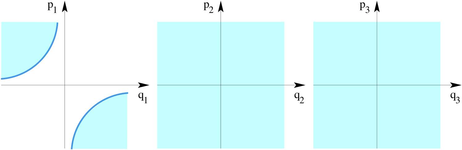
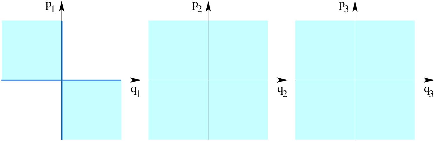
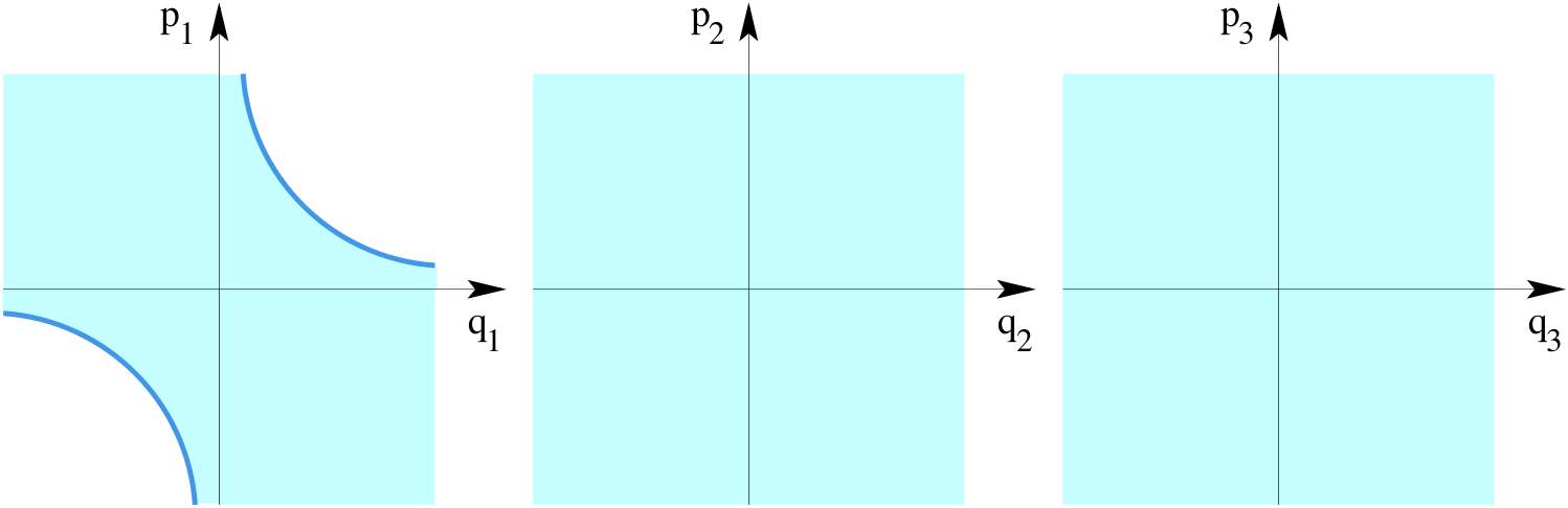
Figure 1: Projection of energy surfaces (turquoise regions) to the planes of the normal form coordinates. The energy surface have energy $h<0$ (top panel), $h=0$ (middle panel), $h>0$ (bottom panel) .

At $h=0$, the formerly disconnected components merge (the energy surface bifurcates), and for $h>0$, the energy surface has locally the structure of a spherical cylinder, $\mathbb{S}^{2n-2}\times\mathds{R}$. Its projection to the plane of the saddle coordinates now includes the origin. In the first and third quadrants it is bounded by the two branches of the hyperbola, $q_{1}p_{1}=I>0$, where $I$ is again given implicitly by the energy equation with all centre actions equal to zero, but now with an energy greater than $0$: $K_{\text{NF}}(I,0,\dots,0)=h>0$. The projections to the planes of the centre coordinates are again unbounded. This is illustrated in the bottom panel of Fig. 1.

The dividing surface, and reacting and nonreacting trajectories: On an energy surface with $h>0$, we define the dividing surface by $q_{1}=p_{1}$. This gives a $(2n-2)$-sphere which we denote by ${\mathbb{S}_{\text{ds}}^{2n-2}(h)}$. Its projection to the saddle coordinates simply gives a line segment through the origin which joins the boundaries of the projection of the energy surface, as shown in Fig. 2. The projections of the dividing surface to the planes of the centre coordinates are bounded by circles $(p_{k}^{2}+q_{k}^{2})/2=J_{k}$, $k=2,\dots,d$, where $J_{k}$ is determined by the energy equation with the other centre actions, $J_{l}$, $l\neq k$, and the saddle integral, $I$, set equal to zero. The dividing surface divides the energy surface into two halves, $p_{1}-q_{1}>0$ and $p_{1}-q_{1}<0$, corresponding to reactants and products.

As mentioned above, trajectories project to hyperbolae in the plane of the saddle coordinates, and to circles in the planes of the centre coordinates. The sign of $I$ determines whether a trajectory is nonreacting or reacting, see Fig. 2. Trajectories which have $I<0$ are nonreactive and for one branch of the hyperbola $q_{1}p_{1}=I$ they stay on the reactants side and for the other branch they stay on the products side; trajectories with $I>0$ are reactive, and for one branch of the hyperbola $q_{1}p_{1}=I$ they react in the forward direction, i.e., from reactants to products, and for the other branch they react in the backward direction, i.e., from products to reactants. The projections of reactive trajectories to the planes of the centre coordinates are always contained in the projections of the dividing surface. In this, and other ways, the geometry of the reaction is highly constrained. There is no analogous restriction on the projections of nonreactive trajectories to the centre coordinates.

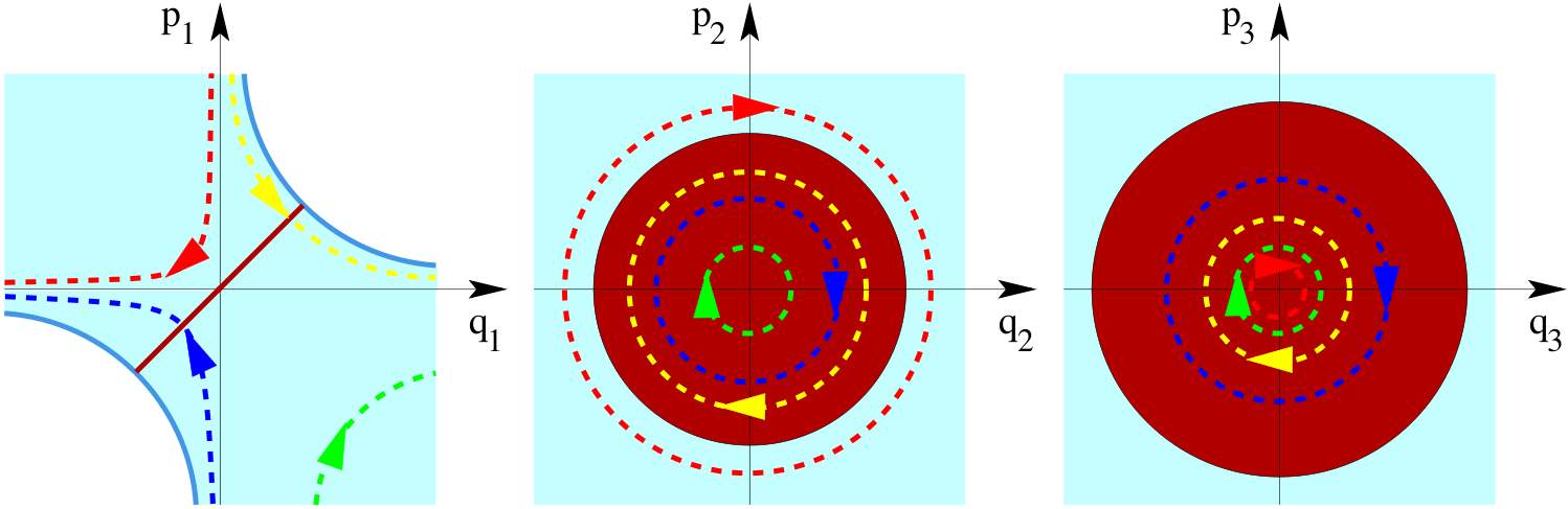
Figure 2: Projection of the dividing surface and reacting and nonreacting trajectories to the planes of the normal form coordinates. In the plane of the saddle coordinates, the projection of the dividing surface is the dark red diagonal line segment, which has $q_{1}=p_{1}$. In the planes of the centre coordinates, the projections of the dividing surface are the dark red discs. Forward and backward reactive trajectories (yellow and blue) project to the first and third quadrant in the plane of the saddle coordinates, respectively, and pass through the dividing surface. The red and green curves mark nonreactive trajectories on the reactant side ($p_{1}-q_{1}>0$), and on the product side ($p_{1}-q_{1}<0$), of the dividing surface, respectively. The turquoise regions indicate the projections of the energy surface.

The normally hyperbolic invariant manifold (NHIM) and its relation to the ‘activated complex’: On an energy surface with $h>0$, the NHIM is given by $q_{1}=p_{1}=0$. The NHIM has the structure of a $(2n-3)$-sphere, which we denote by ${\mathbb{S}_{\text{NHIM}}^{2n-3}(h)}$. The NHIM is the equator of the dividing surface; it divides it into two “hemispheres”: the forward dividing surface, which has $q_{1}=p_{1}>0$, and the backward dividing surface, which has $q_{1}=p_{1}<0$. The forward and backward dividing surfaces have the structure of $(2n-2)$-dimensional balls, which we denote by ${B_{\text{ds,\,f}}^{2n-2}(h)}$ and ${B_{\text{ds,\,b}}^{2n-2}(h)}$, respectively. All forward reactive trajectories cross ${B_{\text{ds,\,f}}^{2n-2}(h)}$; all backward reactive trajectories cross ${B_{\text{ds,\,b}}^{2n-2}(h)}$. Since $q_{1}=p_{1}=0$ in the equations of motion (8) implies that $\dot{q}_{1}=\dot{p}_{1}=0$, the NHIM is an invariant manifold, i.e., trajectories started in the NHIM stay in the NHIM for all time. The system resulting from $q_{1}=p_{1}=0$ is an invariant subsystem with one degree of freedom less than the full system. In fact, $q_{1}=p_{1}=0$ defines the centre manifold associated with the saddle-centre-$\cdots$-centre equilibrium point, and the NHIM at an energy $h$ greater than the energy of the quilibrium point is given by the intersection of the centre manifold with the energy surface of this energy $h$ [Uzer et al.(2002), Waalkens & Wiggins(2004)].

This invariant subsystem with one degree of freedom less than the full system is the “activated complex” (in phase space), located between reactants and products. The NHIM can be considered to be the energy surface of the activated complex. In particular, all trajectories in the NHIM have $I=0$.

The equations of motion (8) also show that $\dot{p}_{1}-\dot{q}_{1}<0$ on the forward dividing surface ${B_{\text{ds,\,f}}^{2n-2}(h)}$, and $\dot{p}_{1}-\dot{q}_{1}>0$ on the backward dividing surface ${B_{\text{ds,\,b}}^{2n-2}(h)}$. Hence, except for the NHIM, which is is an invariant manifold, the dividing surface is everywhere transverse to the Hamiltonian flow. This means that a trajectory, after having crossed the forward or backward dividing surface, ${B_{\text{ds,\,f}}^{2n-2}(h)}$ or ${B_{\text{ds,\,b}}^{2n-2}(h)}$, respectively, must leave the neighbourhood of the dividing surface before it can possibly cross it again. Indeed, such a trajectory must leave the local region in which the normal form is valid before it can possibly cross the dividing surface again.

The NHIM has a special structure: due to the conservation of the centre actions, it is filled, or foliated, by invariant $(n-1)$-dimensional tori, $\mathds{T}^{n-1}$. More precisely, for $d=3$ degrees of freedom, each value of $J_{2}$ implicitly defines a value of $J_{3}$ by the energy equation $K_{\text{NF}}(0,J_{2},J_{3})=h$. For three degrees of freedom, the NHIM is thus foliated by a one-parameter family of invariant 2-tori. The end points of the parameterization interval correspond to $J_{2}=0$ (implying $q_{2}=p_{2}=0$) and $J_{3}=0$ (implying $q_{3}=p_{3}=0$), respectively. At the end points, the 2-tori thus degenerate to periodic orbits, the so-called Lyapunov periodic orbits.

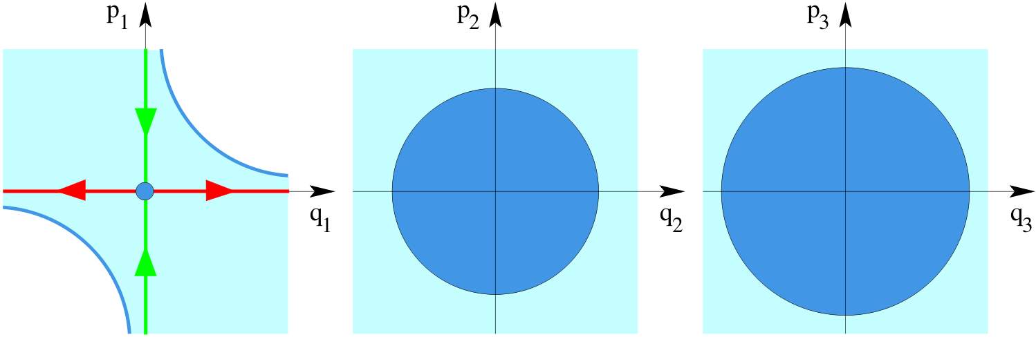
Figure 3: The projection of the NHIM and the local parts of its stable and unstable manifolds, $W^{\text{s}}(h)$ and $W^{u}(h)$, to the planes of the normal form coordinates. In the plane of the saddle coordinates, the projection of the NHIM is the origin marked by the blue bold point, and the projection of $W^{\text{s}}(h)$ and $W^{u}(h)$ are the $p_{1}$-axis and $q_{1}$-axis, respectively. $W^{\text{s}}(h)$ consists of the forward and backward branches $W_{\text{f}}^{\text{s}}(h)$ and $W_{\text{b}}^{\text{s}}(h)$, which have $p_{1}>0$ and $p_{1}<0$, respectively; $W^{\text{u}}(h)$ consists of $W_{\text{f}}^{\text{u}}(h)$ and $W_{\text{b}}^{\text{u}}(h)$, which have $q_{1}>0$ and $q_{1}<0$, respectively. In the plane of the centre coordinates, the projections of the NHIM, $W^{\text{s}}(h)$, and $W^{\text{u}}(h)$ (the blue circular discs) coincide with the projection of the dividing surface in Fig. 2. The turquoise regions mark the projections of the energy surface.

The stable and unstable manifolds of the NHIM forming the phase space conduits for reactions: Since the NHIM is of saddle stability type, it has stable and unstable manifolds, $W^{\text{s}}(h)$ and $W^{\text{u}}(h)$. The stable and unstable manifolds have the structure of spherical cylinders, $\mathbb{S}^{2n-3}\times\mathds{R}$. Each of them consists of two branches: the “forward branches”, which we denote by $W_{f}^{s}(h)$ and $W_{\text{f}}^{\text{u}}(h)$, and the “backward branches”, which we denote by $W_{\text{b}}^{\text{s}}(h)$ and $W_{\text{b}}^{\text{u}}(h)$. In terms of the normal form coordinates, $W_{\text{f}}^{\text{s}}(h)$ is given by $q_{1}=0$ with $p_{1}>0$, $W_{\text{f}}^{\text{u}}(h)$ is given by $p_{1}=0$ with $q_{1}>0$, $W_{b}^{s}(h)$ is given by $q_{1}=0$ with $p_{1}<0$, and $W_{b}^{u}(h)$ is given by $p_{1}=0$ with $q_{1}<0$, see Fig. 3. Trajectories on these manifolds have $I=0$.

Since the stable and unstable manifolds of the NHIM are of one less dimension than the energy surface, they enclose volumes of the energy surface. We call the union of the forward branches, $W_{f}^{s}(h)$ and $W_{\text{f}}^{\text{u}}(h)$, the forward reactive spherical cylinder and denote it by $W_{\text{f}}(h)$. Similarly, we define the backward reactive spherical cylinder, $W_{\text{b}}(h)$, as the union of the backward branches, $W_{\text{b}}^{\text{s}}(h)$ and $W_{\text{b}}^{\text{u}}(h)$.

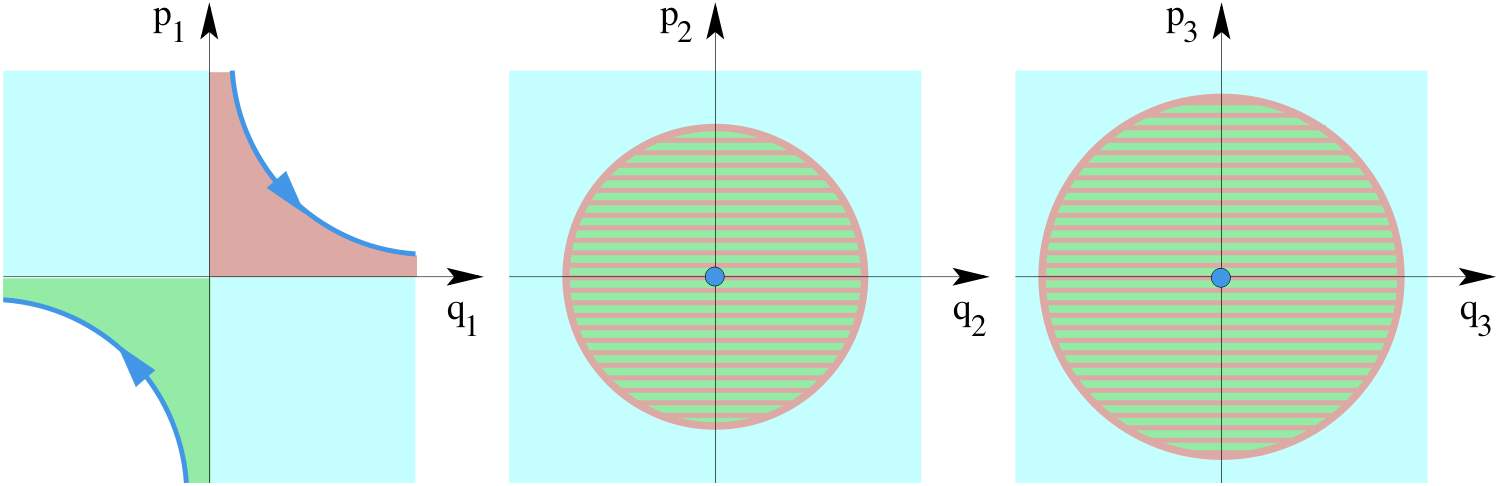
Figure 4: Projections of the reactive volumes enclosed by the forward and backward reactive spherical cylinders, $W_{\text{f}}(h)$ and $W_{\text{b}}(h)$, and the forward and backward reactions paths, to the planes of the normal form coordinates. The volumes enclosed by $W_{\text{f}}(h)$ and $W_{\text{b}}(h)$ project to the dark pink and green regions in the first and third quadrant in the plane of the saddle coordinates, respectively. These volumes project to the dark green/dark pink brindled disks in the planes of the centre coordinates, where their projections coincide with the projection of the NHIM and the dividing surface in Figs. 2 and 3. The forward and backward reaction paths project to the two branches of a hyperbola marked blue in the first and third quadrant in the plane of the saddle coordinates, respectively, and to the origins (bold blue points) in the planes of the centre coordinates. The turquoise regions mark the projections of the energy surface.

The reactive volumes enclosed by $W_{f}(h)$ and $W_{b}(h)$ are shown in Fig. 4 as their projections to the normal form coordinate planes. In the plane of the saddle coordinates, the reactive volume enclosed by $W_{f}(h)$ projects to the first quadrant. This projection is bounded by the corresponding hyperbola $q_{1}p_{1}=I$, with $I$ obtained from $K_{\text{NF}}(I,0,\dots,0)=h$. Likewise, $W_{b}(h)$ projects to the third quadrant in the $(q_{1},p_{1})$-plane. $W_{f}(h)$ encloses all forward reactive trajectories; $W_{b}(h)$ encloses all backward reactive trajectories. All nonreactive trajectories are contained in the complement.

Forward and backward reaction paths: The local geometry of $W_{\text{f}}(h)$ and $W_{\text{b}}(h)$ suggests a natural definition of dynamical forward and backward reaction paths as the unique paths in phase space obtained by putting all of the energy of a reacting trajectory into the reacting mode, i.e., setting $q_{2}=\dots=q_{n}=p_{2}=\dots=p_{n}=0$. This gives the two branches of the hyperbola $q_{1}p_{1}=I$, with $I$ obtained from $K_{\text{NF}}(I,0,\dots,0)=h$, which in phase space are contained in the plane of the saddle coordinates, see Fig. 4. This way, the forward (respectively, backward) reaction path can be thought of as the “centre curve” of the relevant volume enclosed by the forward (resp., backward) reactive spherical cylinder $W_{\text{f}}(h)$ (resp., $W_{\text{b}}(h)$). These reaction paths are the special reactive trajectories which intersect the dividing surface at the “poles” (in the sense of North and South poles, where $q_{1}=p_{1}$ assumes its maximum and minimum value on the dividing surface).

The Transmission Time through the Transition State Region: The normal form coordinates provide a way of computing the time for all trajectories to cross the transition region. We illustrate this with a forward reacting trajectory (a similar argument and calculation can be applied to backward reacting trajectories). We choose the boundary for the entrance to the reaction region to be $p_{1}-q_{1}=c$ for some constant $c>0$, i.e., initial conditions which lie on the reactant side of the transition state, and the boundary for exiting the reaction region to be $p_{1}-q_{1}=-c$ on the product side. We now compute the time of flight for a forward reacting trajectory with initial condition on $p_{1}-q_{1}=c$ to reach $p_{1}-q_{1}=-c$ on the product side. The solutions are $q_{1}(t)=q_{1}(0)\exp(\Lambda(I,J_{2},\dots,J_{n})t)$ and $p_{1}(t)=p_{1}(0)\exp(-\Lambda(I,J_{2},\dots,J_{n})t)$ (see (8)), where $\Lambda(I,J_{2},\dots,J_{n})$ is determined by the initial conditions. This gives the time of flight as

$$T=\left(\Lambda(I,J_{2},\dots,J_{n})\right)^{-1}\ln\left(\frac{p_{1}(0)}{q_{1}(0)}\right).$$ (11)

The time diverges logarithmically as $q_{1}(0)\rightarrow 0$, i.e., the closer the trajectory starts to the boundary $W_{\text{f}}(h)$. It is not difficult to see that the time of flight is shortest for the centre curve of the volume enclosed by $W_{\text{f}}(h)$, i.e., the trajectory which traverses the transition state region fastest is precisely our forward reaction path. A similar construction applies to backward reactive trajectories.

In fact, the normal form can be used to map trajectories through the transition state region, i.e. the phase space point at which a trajectory enters the transition state region can be mapped analytically to the phase space point at which the trajectories exits the transition state region.

2.3 The foliation of the reaction region by Lagrangian submanifolds

The existence of the $n$ integrals of motion, $(I,J_{2},\ldots,J_{n})$, induce phase space structures which lead to further constraints on the trajectories in addition to the ones described above. In order to describe these structures and the resulting constraints it is useful to introduce the so called momentum map, ${\cal M}$ [Guillemin(1994), Marsden & Ratiu(1999)] which maps a point $(q_{1},\ldots,q_{n},p_{1},\ldots,p_{n})$ in the phase space $\mathds{R}^{n}\times\mathds{R}^{n}$ to the $n$ integrals evaluated at this point:

$${\cal M}:\mathds{R}^{n}\times\mathds{R}^{n}\to\mathds{R}^{n}\,,\quad(q_{1},\ldots,q_{n},p_{1},\ldots,p_{n})\mapsto(I,J_{2},\ldots,J_{n})\,.$$ (12)

The preimage of a value for the constants of motion $(I,J_{2},\ldots,J_{n})$ under ${\cal M}$ is called a fibre. A fibre thus corresponds to the common level set of the integrals in phase space.

A point $(q_{1},\ldots,q_{n},p_{1},\ldots,p_{n})$ is called a regular point of the momentum map if the linearisation of the momentum map, D$\mathcal{M}$, has full rank $n$ at this point, i.e., if the gradients of the $n$ integrals $I$, $J_{k}$, $k=2,\ldots,n$, with respect to the phase space coordinates $(q,p)$ are linearly independent at this point. If the rank of D$\mathcal{M}$ is less than $n$ then the point is called irregular. A fibre is called regular if it consists of regular points only. Else it is called an irregular fibre. In fact almost all fibres are regular. They are $n$-dimensional manifolds given by the Cartesian product of an hyperbola $q_{1}p_{1}=I$ in the saddle plane $(q_{1},p_{1})$ and $n-1$ circles $\mathbb{S}^{1}$ in the centre planes $(q_{k},p_{k})$, $k=2,\ldots,n$. Since the hyperbola $q_{1}p_{1}=I$ consists of two branches each of which have the topology of a line $\mathds{R}$, the regular fibres consist of two disjoint toroidal cylinders, $\mathds{T}^{n-1}\times\mathds{R}$, which are the Cartesian products of a $(n-1)$-dimensional torus and a line. We denote these toroidal cylinders by

$$\Lambda^{+}_{I,J_{2},\ldots,J_{n}}=\{(q,p)\in\mathds{R}^{2n}\,:\,p_{1}q_{1}=I,\,\frac{1}{2}\big{(}p_{2}^{2}+q_{2}^{2}\big{)}=J_{2}\,,\ldots\,,\frac{1}{2}\big{(}p_{n}^{2}+q_{n}^{2}\big{)}=J_{n}\,,q_{1}>0\}$$ (13)

and

$$\Lambda^{-}_{I,J_{2},\ldots,J_{n}}=\{(q,p)\in\mathds{R}^{2n}\,:\,p_{1}q_{1}=I,\,\frac{1}{2}\big{(}p_{2}^{2}+q_{2}^{2}\big{)}=J_{2}\,,\ldots\,,\frac{1}{2}\big{(}p_{n}^{2}+q_{n}^{2}\big{)}=J_{n}\,,q_{1}<0\}\,.$$ (14)

$\Lambda^{+}_{I,J_{2},\ldots,J_{d}}$ and $\Lambda^{-}_{I,J_{2},\ldots,J_{d}}$ are Lagrangian manifolds [Arnold(1978)]. The Lagrangian manifolds consists of all trajectories which have the same constants of motion. In particular the Lagrangian manifolds are invariant, i.e. a trajectory with initial condition on a Lagrangian manifold will stay in the Lagrangian manifold for all time. For $I<0$, the Lagrangian manifolds $\Lambda^{-}_{I,J_{2},\ldots,J_{n}}$ and $\Lambda^{+}_{I,J_{2},\ldots,J_{n}}$ consist of nonreactive trajectories in the reactants resp. products components of the energy surface. For $I>0$, $\Lambda^{+}_{I,J_{2},\ldots,J_{n}}$ consists of forward reactive trajectories, and $\Lambda^{-}_{I,J_{2},\ldots,J_{n}}$ consists of backward reactive trajectories.

We will discuss the irregular fibres in more detail in Sec. 4.

2.4 Implications for the original system

The normalization procedure proceeds via formal power series manipulations whose input is a Taylor expansion of the original Hamiltonian, $H$, necessarily up to some finite order, $M$, in homogeneous polynomials. For a particular application, this procedure naturally necessitates a suitable choice of the order, $M$, for the normalization, after which one must make a restriction to some local region, $\mathcal{L}$, about the equilibrium point in which the resulting computations achieve some desired accuracy. Hence, the accuracy of the normal form as a power series expansion truncated at order $M$ in a neighborhood $\mathcal{L}$ is determined by comparing the dynamics associated with the normal form with the dynamics of the original system. There are several independent tests that can be carried out to verify accuracy of the normal form. Straightforward tests that we use are the following:

• Examine how the integrals associated with the normal form change on trajectories of the full Hamiltonian (the integrals will be constant on trajectories of the normal form).

• Check invariance of the different invariant manifolds (i.e. the NHIM and its stable and unstable manifolds) with respect to trajectories of the full Hamiltonian.

Both of these tests will require us to use the transformations between the original coordinates and the normal form coordinates. Specific examples where $M$, $\mathcal{L}$ and accuracy of the normal forms are considered can be found in [Waalkens et al.(2004a), Waalkens et al.(2004b), Waalkens et al.(2005a), Waalkens et al.(2005b), Waalkens et al.(2005c)].

3 Models of the local phase space structures for 2-DoF systems

In the discussion of the phase space structures governing reaction type dynamics in Sec. 2.2 we visualized these structures by projecting them to the 2-dimensional planes of the coordinates and conjugate momenta of the normal form. The topology of the phase space structures and the interrelationship between them is to a large extent obscured in these projection because of the lacking injectivity of the projections. For $n=2$ DoFhowever, a surface of constant energy containing the phase space structures is three-dimensional. For this case, it is therefore possible to visualize the phase space structures in three-dimensional space. In this section we will develop three models to explicitly implement such visualizations. Our discussion will be in the context of linear Hamiltonian systems since they allow us to describe the phase space structures in terms of explicit formulae. The influence of nonlinear terms is discussed in Sec. 3.4.

Therefore we begin by considering the quadratic Hamiltonian

$$H(x,y,p_{x},p_{y})=\frac{\lambda}{2}\big{(}p_{x}^{2}-x^{2}\big{)}+\frac{\omega}{2}\big{(}p_{y}^{2}+y^{2}\big{)}$$ (15)

with $\lambda,\omega>0$.

This gives the linear Hamiltonian vector field

$$\dot{x} = \phantom{-}\frac{\partial H}{\partial p_{x}}=\lambda p_{x},$$ (16)

$$\dot{p}_{x} = -\frac{\partial H}{\partial x}=\lambda x,$$ (17)

$$\dot{y} = \phantom{-}\frac{\partial H}{\partial p_{y}}=\omega p_{y},$$ (18)

$$\dot{p}_{y} = -\frac{\partial H}{\partial y}=-\omega y,\,.$$ (19)

The Hamiltonian (15) is already in normal form. To keep the notation simple we will not specifically indicate this by a subscript NF. In fact we have

$$H(x,y,p_{x},p_{y})=K(I,J)=\lambda I+\omega J\,,$$ (20)

where $I$ and $J$ are the integrals given in (6)) and (7), respectively.

For a fixed energy $h$, the three dimensional energy surface is given by the level set of the Hamiltonian (15) as follows:

$$\Sigma(h)=\{(x,y,p_{x},p_{y})\in\mathds{R}^{4}\,:\,\lambda\big{(}p_{x}^{2}-x^{2}\big{)}+\omega\big{(}p_{y}^{2}+y^{2}\big{)}=2h\}\,.$$ (21)

We rewrite the energy equation in the form

$$\lambda p_{x}^{2}+\omega p_{y}^{2}+\omega y^{2}=2h+\lambda x^{2}\,,$$ (22)

and fix $x$ such that the right hand side of this equation is positive. Note that if $h>0$ the right hand side will be positive for any fixed $x\in\mathds{R}$, while if $h<0$ it will be positive only for $|x|>\sqrt{-2h/\lambda}$, i.e. for $x$ sufficiently small or large. For such an $x$, Eq. (22) defines an ellipsoid in the three-dimensional Euclidean space, $\mathds{R}^{3}$, with coordinates $(p_{x},p_{y},y)$. This ellipsoid is rotationally symmetric about the $p_{x}$-axis. It has two semi-axes of length $\big{(}(2h+\lambda x^{2})/\omega\big{)}^{1/2}$ and one semi-axis of length $\big{(}(2h+\lambda x^{2})/\lambda\big{)}^{1/2}$. Topologically, this is a two-dimensional sphere, $\mathbb{S}^{2}$, which we denote by $\mathbb{S}_{x}^{2}(h)$, i.e.

$$\mathbb{S}^{2}_{x}(h)=\{(p_{x},p_{y},y)\in\mathds{R}^{3}\,:\,\lambda p_{x}^{2}+\omega\big{(}p_{y}^{2}+y^{2}\big{)}=2h+\lambda x^{2}\}\,.$$ (23)

The energy surface thus appears to have the structure of a one-parameter family of two-dimensional spheres parametrized by $x$, where the ‘radius’ (the length of the shortest semi-axis of the ellipsoid (22)) can shrink to zero if $h<0$. The three models of the energy surface and the phase space structures contained in it that we present in the following differ by the way of representing the 2-spheres $\mathbb{S}^{2}_{x}(h)$. For clarity, let us summarize the phase space structures discussed in Sec. 2 for the Hamiltonian (15) before we proceed. We will restrict ourselves to the case $h>0$.

The dividing surface is obtained by setting $x=0$ on the energy surface. This gives the two-dimensional sphere

$${\mathbb{S}_{\text{ds}}^{2}(h)}=\Sigma(h)\cap\{x=0\}=\{(x,y,p_{x},p_{y})\in\mathds{R}^{4}\,:\,\lambda p_{x}^{2}+\omega\big{(}p_{y}^{2}+y^{2}\big{)}=2h,\,x=0\}\,.$$ (24)

For the 2-DoF  case, the NHIM is an unstable periodic orbit (the Lyapunov periodic orbit associated with the saddle point). For the Hamiltonian (15), it is obtained by setting $x=0$ and $p_{x}=0$ on the energy surface. This gives the circle

$${\mathbb{S}_{\text{NHIM}}^{1}(h)}=\Sigma(h)\cap\{x=0,\,p_{x}=0\}=\{(x,y,p_{x},p_{y})\in\mathds{R}^{4}\,:\,\omega\big{(}p_{y}^{2}+y^{2}\big{)}=2h,\,x=0,\,p_{x}=0\}\,.$$ (25)

The NHIM divides the dividing surface, ${\mathbb{S}_{\text{ds}}^{2}(h)}$, into the forward hemisphere

$${B_{\text{ds,\,f}}^{2}(h)}=\Sigma(h)\cap\{x=0,\,p_{x}>0\}=\{(x,y,p_{x},p_{y})\in\mathds{R}^{4}\,:\,p_{x}=\sqrt{\big{(}2h-\omega\big{(}p_{y}^{2}+y^{2}\big{)}\big{)}/\lambda},\,x=0\}$$ (26)

and the backward hemisphere

$${B_{\text{ds,\,b}}^{2}(h)}=\Sigma(h)\cap\{x=0,\,p_{x}<0\}=\{(x,y,p_{x},p_{y})\in\mathds{R}^{4}\,:\,p_{x}=-\sqrt{\big{(}2h-\omega\big{(}p_{y}^{2}+y^{2}\big{)}\big{)}/\lambda},\,x=0\}\,,$$ (27)

which are two dimensional balls or disks. The stable manifold $W^{s}$ of ${\mathbb{S}_{\text{NHIM}}^{1}(h)}$ consists of the forward branch

$$W^{s}_{\text{f}}=\Sigma(h)\cap\{x=-p_{x},\,x<0\}=\{(x,y,p_{x},p_{y})\in\mathds{R}^{4}\,:\,\omega\big{(}p_{y}^{2}+y^{2}\big{)}=2h,\,x=-p_{x},\,x<0\}$$ (28)

and the backward branch

$$W^{s}_{\text{b}}=\Sigma(h)\cap\{x=-p_{x},\,x>0\}=\{(x,y,p_{x},p_{y})\in\mathds{R}^{4}\,:\,\omega\big{(}p_{y}^{2}+y^{2}\big{)}=2h,\,x=-p_{x},\,x>0\}\,.$$ (29)

Similarly, the unstable manifold $W^{u}$ of ${\mathbb{S}_{\text{NHIM}}^{1}(h)}$ consists of the forward branch

$$W^{u}_{\text{f}}=\Sigma(h)\cap\{x=p_{x},\,x>0\}=\{(x,y,p_{x},p_{y})\in\mathds{R}^{4}\,:\,\omega\big{(}p_{y}^{2}+y^{2}\big{)}=2h,\,x=p_{x},\,x>0\}$$ (30)

and the backward branch

$$W^{u}_{\text{b}}=\Sigma(h)\cap\{x=p_{x},\,x<0\}=\{(x,y,p_{x},p_{y})\in\mathds{R}^{4}\,:\,\omega\big{(}p_{y}^{2}+y^{2}\big{)}=2h,\,x=p_{x},\,x<0\}\,.$$ (31)

Finally, the forward and backward reaction paths are obtained from putting all the energy in the $x$ DoF. This gives the lines

$$\Sigma(h)\cap\{y=p_{y}=0,\,p_{x}>0\}=\{(x,y,p_{x},p_{y})\in\mathds{R}^{4}\,:\,p_{x}=\sqrt{(2h+\lambda x)/\lambda},\,y=p_{y}=0\}$$ (32)

for the forward reaction path, and

$$\Sigma(h)\cap\{y=p_{y}=0,\,p_{x}<0\}=\{(x,y,p_{x},p_{y})\in\mathds{R}^{4}\,:\,p_{x}=-\sqrt{(2h+\lambda x)/\lambda},\,y=p_{y}=0\}$$ (33)

for the backward reaction path.

Note that the energy surface (21), the phase space structures (24)-(33) and also the Lagrangian cylinders defined in (13) and (14) are invariant under the $\mathbb{S}^{1}$ symmetry action

$$(x,y,p_{x},p_{y})\to(x,\mathrm{e}^{-\mathrm{i}\varphi}y,p_{x},\mathrm{e}^{-\mathrm{i}\varphi}p_{y})\,,\quad\varphi\in\mathbb{S}^{1}\,.$$ (34)

3.1 Model I: projection of 2-spheres to their equatorial planes

The main idea of the first model is to view the 2-sphere (23) as consisting of two hemispheres and an equator, i.e. as the disjoint union of two open two-dimensional disks or balls, $B^{2}$, and a circle, or equivalently one-dimensional sphere, $\mathbb{S}^{1}$, and using parametrizations of these geometric structures to parametrize the energy surface.

The decomposition of a 2-sphere, $\mathbb{S}^{2}$, in terms of 2-balls and a circle is familiar from visualizing the surface of the Earth by drawing two filled-in disks ($B^{2}$), one each for the Northern and Southern hemispheres, and identifying the boundaries of the two disks,

$$\mathbb{S}^{2}\equiv B^{2}_{\text{North}}\cup\mathbb{S}^{1}_{\text{Equator}}\cup B^{2}_{\text{South}},$$ (35)

which we illustrate in Fig. 5.

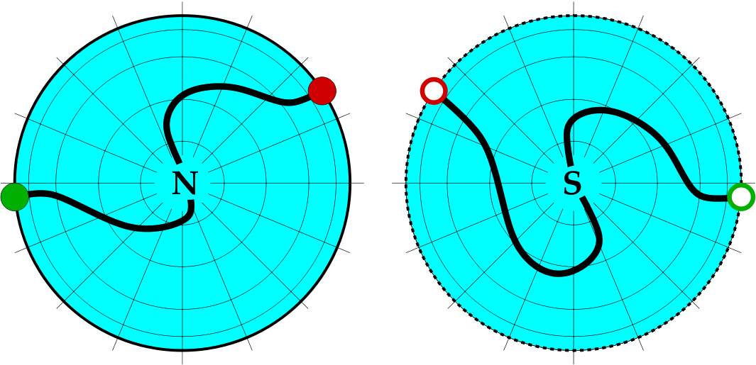
Figure 5: A model of the sphere $\mathbb{S}^{2}$ formed by taking two open discs ($2$-balls) $B^{2}_{\text{North}}$ and $B^{2}_{\text{South}}$ and identifying points on their boundaries; the “equator” $\mathbb{S}^{1}_{\text{Equator}}$. Also shown is the representation of a smooth closed curve on $\mathbb{S}^{2}$ which passes through the North and South poles, $N$ and $S$; the points at which the representation of the curve “jumps” from one disc in the model to the other disc are marked by dots.

For the 2-spheres $\mathbb{S}^{2}_{x}(h)$ in Eq. (23), we define the decomposition (35) as

$$\mathbb{S}^{2}_{x}(h)=B^{2}_{+,x}(h)\cup\mathbb{S}^{1}_{0,x}(h)\cup B^{2}_{-,x}(h)\,,$$ (36)

where

$$B^{2}_{+,x}(h) = \{(p_{x},p_{y},y)\in\mathds{R}^{3}\,:\,\omega\big{(}p_{y}^{2}+y^{2}\big{)}<2h-\lambda x^{2},\,p_{x}=\phantom{-}\sqrt{(2h+\lambda x^{2}-\omega p_{y}^{2}-\omega y^{2})/\lambda}>0\}\,,$$ (37)

$$B^{2}_{-,x}(h) = \{(p_{x},p_{y},y)\in\mathds{R}^{3}\,:\,\omega\big{(}p_{y}^{2}+y^{2}\big{)}<2h-\lambda x^{2},\,p_{x}=-\sqrt{(2h+\lambda x^{2}-\omega p_{y}^{2}-\omega y^{2})/\lambda}<0\}\,,$$ (38)

$$\mathbb{S}^{1}_{0,x}(h) = \{(p_{x},p_{y},y)\in\mathds{R}^{3}\,:\,\omega\big{(}p_{y}^{2}+y^{2}\big{)}=2h-\lambda x^{2},\,p_{x}=0\}\,.$$ (39)

We can view the manifolds $B^{2}_{+,x}(h)$ and $B^{2}_{-,x}(h)$ as graphs of the functions

$${\mathcal{P}}_{\pm,x}:\tilde{B}^{2}_{x}(h)\rightarrow\mathds{R}\,,\quad(y,p_{y})\mapsto\pm\sqrt{(2h+\lambda x^{2}-\omega p_{y}^{2}-\omega y^{2})/\lambda}\,,$$ (40)

where the domains are the circular disks

$$\tilde{B}^{2}_{x}(h)=\{(p_{y},y)\in\mathds{R}^{2}\,:\,\omega\big{(}p_{y}^{2}+y^{2}\big{)}<2h+\lambda x^{2}\}\subset\mathds{R}^{2}\,.$$ (41)

The graphs ‘join’ at the equator $\mathbb{S}^{1}_{0,x}(h)$. In order to geometrically visualize $\mathbb{S}^{2}_{x}(h)$ we take two copies of the circular disks $\tilde{B}^{2}_{x}(h)$ in the $(y,p_{y})$-plane where $p_{x}$ is given by the function ${\mathcal{P}}_{+,x}$ on one copy which we denote by $\tilde{B}^{2}_{+,x}(h)$ and the function ${\mathcal{P}}_{-,x}$ on the other copy which we denote by $\tilde{B}^{2}_{-,x}(h)$. $\tilde{B}^{2}_{\pm,x}(h)$ thus denote the images of $B^{2}_{\pm,x}(h)$ under the projection

$$\pi_{p_{x}\,x}:B^{2}_{\pm,x}(h)\to\mathds{R}^{2}\,,\quad(p_{x},p_{y},y)\mapsto(y,p_{y})\,,$$ (42)

see Fig. 6. Along the boundaries of $\tilde{B}^{2}_{+,x}(h)$ and $\tilde{B}^{2}_{-,x}(h)$ we have $p_{x}=0$, and the points on the boundaries which have the same $(y,p_{y})$ are identified.

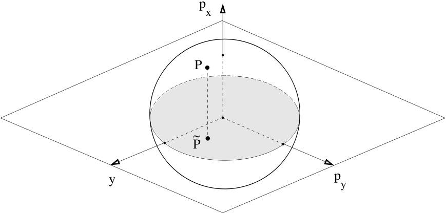
Figure 6: Model I: projection of $\mathbb{S}^{2}_{x}(h)$ to the $(y,p_{y})$-plane.

The first model (Model I) of the energy surface and the phase space structures contained in it is obtained from defining a map from the energy surface $\Sigma(h)$ to $\mathds{R}^{3}$ using the projections $\pi_{p_{x}\,x}$, $x\in\mathds{R}$, in (42) to map points $(x,y,p_{x},p_{y})\in\Sigma(h)$ according to

$$F^{\text{I}}:(x,y,p_{x},p_{y})\mapsto(x,\pi_{p_{x}\,x}(p_{x},p_{y},y))=(x,y,p_{y})\,.$$ (43)

The map $F^{\text{I}}$ is singular along the cylinder given by the union of the circles $\mathbb{S}^{1}_{0,x}(h)$ in (39) with $x\in\mathds{R}$. This singular cylinder is mapped to the quadric

$$\frac{p_{y}^{2}}{2h/\omega}-\frac{x^{2}}{2h/\lambda}+\frac{y^{2}}{2h/\omega}=1$$ (44)

which is a single sheeted hyperboloid that is rotationally symmetric about the $x$ axis. Each point in $(x,y,p_{y})\in\mathds{R}^{3}$ with

$$\frac{p_{y}^{2}}{2h/\omega}-\frac{x^{2}}{2h/\lambda}+\frac{y^{2}}{2h/\omega}<1$$ (45)

has two preimages that differ by the sign of $p_{x}$. We can thus represent the energy surface $\Sigma(h)$ in the three dimensional space, $\mathds{R}^{3}$, in terms of the manifolds

$$\begin{split}\Sigma^{\text{I}}_{\pm}(h)&=\{(x,y,p_{y})\in\mathds{R}^{3}\,:\,x\in\mathds{R},\,(y,p_{y})\in\tilde{B}^{2}_{\pm,x}(h)\}\\ &=\{(x,y,p_{y})\in\mathds{R}^{3}\,:\,\frac{p_{y}^{2}}{2h/\omega}-\frac{x^{2}}{2h/\lambda}+\frac{y^{2}}{2h/\omega}<1\}\,,\end{split}$$ (46)

where $p_{x}=(2h+x^{2}-p_{y}^{2}-y^{2})^{1/2}$ is positive on $\Sigma^{\text{I}}_{+}(h)$ and $p_{x}=-(2h+x^{2}-p_{y}^{2}-y^{2})^{1/2}$ is negative on $\Sigma^{\text{I}}_{-}(h)$. The full energy surface $\Sigma(h)$ is obtained by gluing $\Sigma^{\text{I}}_{\pm}(h)$ along their boundaries (44) where $p_{x}=0$. We show illustrations of $\Sigma^{\text{I}}_{+}(h)$ and $\Sigma^{\text{I}}_{-}(h)$ in the top panels of Fig. 7. As a consequence of the symmetry (34) the components $\Sigma^{\text{I}}_{\pm}(h)$ are both rotationally symmetric about the $x$-axis. It is therefore useful to consider also the intersections of $\Sigma^{\text{I}}_{+}(h)$ and $\Sigma^{\text{I}}_{+}(h)$ (and of the other phase space structures discussed in the following) with the plane $y=0$ as shown in the bottom panels of Fig. 7.

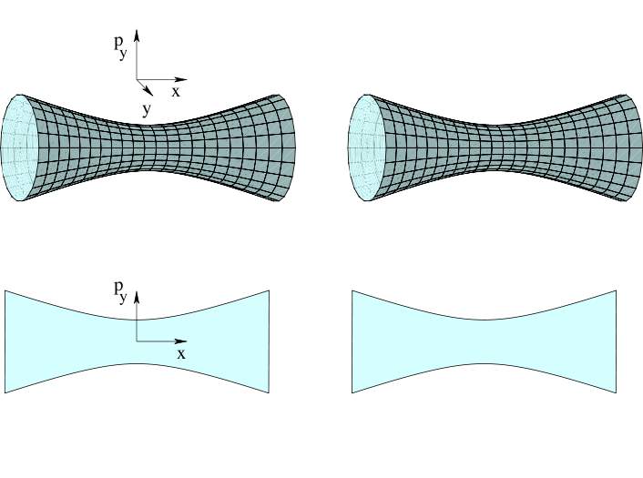
Figure 7: Model I: the energy surface. The orientation of the $x$, $y$ and $p_{y}$ axes is indicated by the dreibein. (Note that the origin of the coordinate system is not the center of the dreibein.) The top left panel shows $\Sigma^{\text{I}}_{+}(h)$; the top left panel shows $\Sigma^{\text{I}}_{-}(h)$. The two panels at the bottom show the intersections of $\Sigma^{\text{I}}_{+}(h)$ and $\Sigma^{\text{I}}_{-}(h)$ with the plane $y=0$.

It is easy to see the wide-narrow-wide geometry of the bottleneck type structure of the energy surface in this representation of the energy surface. The reactants region is on the left, the product regions is on the right.

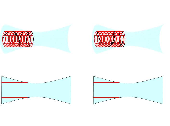
Figure 8: Model I: nonreactive trajectories that stay in the reactants component. The red wireframes in the top panels indicate the two pieces of a Lagrangian cylinder $\Lambda^{-}_{I,J}$ defined in (14) for $I<0$ contained in $\Sigma^{\text{I}}_{+}(h)$ and $\Sigma^{\text{I}}_{-}(h)$, respectively. The black line shows one of the trajectories contained in $\Lambda^{-}_{I,J}$. The red lines in the bottom panels show the intersection of $\Lambda^{-}_{I,J}$ with the plane $y=0$.

In Fig. 8 we show the image under $F^{\text{I}}$ of a Lagrangian cylinder $\Lambda^{-}_{I,J}$ defined in (14) for $I<0$ together with a nonreactive trajectory contained in this cylinder. Note that for a 2-DoF system and given values for the integral $I$ and the energy $h$, the second integral $J$ is fixed by the energy equation $K(I,J)=h$ (see (20)). The trajectory approaches the bottleneck region with positive $p_{x}$ from the reactants component of the energy surface within $\Sigma^{\text{I}}_{+}(h)$ (the left panels of Fig. 8), reaches the boundary (44) of $\Sigma^{\text{I}}_{+}(h)$, where $p_{x}=0$ and the trajectory ‘jumps’ to $\Sigma^{\text{I}}_{-}(h)$ (the right panels in Fig. 8) after which it returns back deeper into the reactants region with $p_{x}<0$.

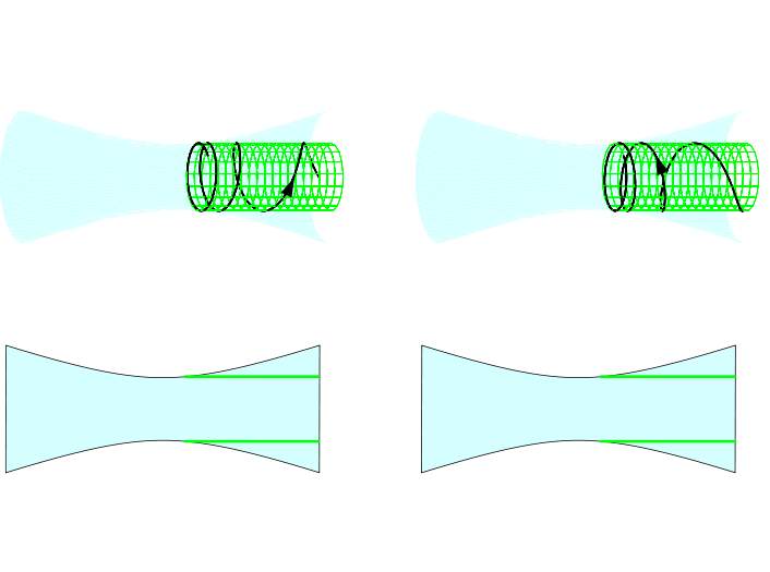
Figure 9: Model I: nonreactive trajectories that stay in the products component. The green wireframes in the top panels indicate the two pieces of a Lagrangian cylinder $\Lambda^{+}_{I,J}$ defined in (13) for $I<0$ contained in $\Sigma^{\text{I}}_{+}(h)$ and $\Sigma^{\text{I}}_{-}(h)$, respectively. The black line shows one of the trajectories contained in $\Lambda^{+}_{I,J}$. The green lines in the bottom panels show the intersection of $\Lambda^{+}_{I,J}$ with the plane $y=0$.

Figure 9 shows the $F^{\text{I}}$ image of a Lagrangian cylinder $\Lambda^{+}_{I,J}$ for $I<0$ together with a trajectory contained in $\Lambda^{+}_{I,J}$. The trajectory approaches the bottleneck region with negative $p_{x}$ from the products side of the energy surface within $\Sigma^{\text{I}}_{-}(h)$ (the right panels of Fig. 9), reaches the boundary (44) of $\Sigma^{\text{I}}_{-}(h)$, where $p_{x}=0$ and the trajectory ‘jumps’ to $\Sigma^{\text{I}}_{+}(h)$ (the left panels in Fig. 9), in which it returns back deeper in to the products region with $p_{x}>0$.

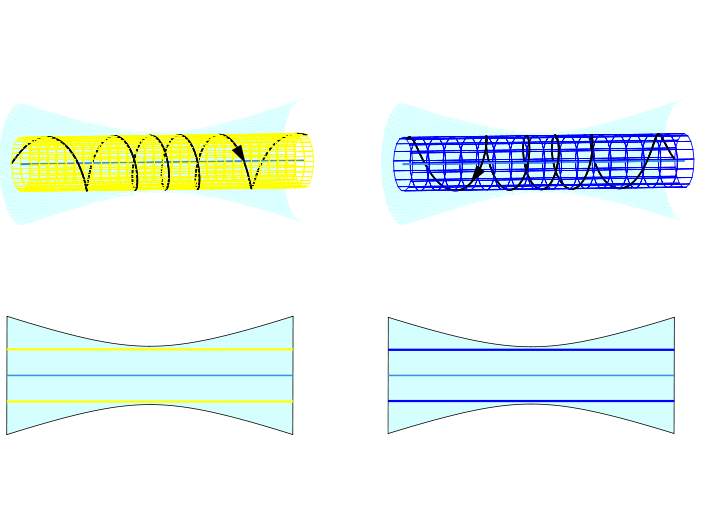
Figure 10: Model I: forward and backward reactive trajectories spiraling about the forward and backward reaction paths, respectively. The yellow wireframe in the top left panel indicates a Lagrangian cylinder $\Lambda^{+}_{I,J}$ with $I>0$ contained in $\Sigma^{\text{I}}_{+}(h)$; the blue wireframe in the top right panel indicates a Lagrangian cylinder $\Lambda^{-}_{I,J}$ with $I>0$ contained in $\Sigma^{\text{I}}_{-}(h)$. The black lines show trajectories contained in the respective cylinders. The blue centerlines show the forward (left) and backward (right) reaction paths. The bottom panels show the intersections of the Lagrangian cylinders with the plane $y=0$ together with the forward and backward reaction paths.

Figure 10 shows the $F^{\text{I}}$ images of Lagrangian cylinders $\Lambda^{-}_{I,J}$ and $\Lambda^{+}_{I,J}$ for $I>0$. For $I>0$, $\Lambda^{+}_{I,J}$ contains forward reactive trajectories which have $p_{x}>0$ and therefore are completely contained in $\Sigma^{\text{I}}_{+}(h)$ (the left panels in Fig. 10), and $\Lambda^{-}_{I,J}$ contains backward reactive trajectories which have $p_{x}<0$ and therefore are completely contained in $\Sigma^{\text{I}}_{-}(h)$ (the right panels in Fig. 10). The forward and backward trajectories spiral about the forward and backward reaction paths which are also shown in Fig. 10.

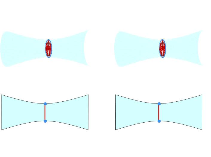
Figure 11: Model I: the dividing surface and the NHIM. The dark red wireframes indicate the two hemispheres ${B_{\text{ds,\,f}}^{2}(h)}$ (top left panel) and ${B_{\text{ds,\,b}}^{2}(h)}$ (top right panel) the dividing surface ${\mathbb{S}_{\text{ds}}^{2}(h)}$. The light blue circle in the top panels shows the periodic orbit ${\mathbb{S}_{\text{NHIM}}^{1}(h)}$. The lower panels show the intersections of ${B_{\text{ds,\,f}}^{2}(h)}$, ${B_{\text{ds,\,b}}^{2}(h)}$ and ${\mathbb{S}_{\text{NHIM}}^{1}(h)}$ with the plane $y=0$.

The images of the dividing surface, ${\mathbb{S}_{\text{ds}}^{2}(h)}$, and the NHIM, ${\mathbb{S}_{\text{NHIM}}^{1}(h)}$, under $F^{\text{I}}$ are shown in Fig. 11. The forward hemisphere ${B_{\text{ds,\,f}}^{2}(h)}$ is contained in $\Sigma^{\text{I}}_{+}(h)$ (the left panels in Fig. 11); the backward hemisphere ${B_{\text{ds,\,b}}^{2}(h)}$ is contained in $\Sigma^{\text{I}}_{-}(h)$ (the right panels in Fig. 11). The periodic orbit ${\mathbb{S}_{\text{NHIM}}^{1}(h)}$ which forms the equator of ${\mathbb{S}_{\text{ds}}^{2}(h)}$ has $p_{x}=0$ and thus runs along the boundaries of $\Sigma^{\text{I}}_{+}(h)$ and $\Sigma^{\text{I}}_{-}(h)$.

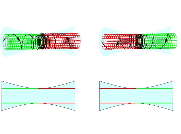
Figure 12: Model I: the stable and unstable manifolds of the NHIM. The wireframes in the top left panel show the branches $W^{s}_{\text{f}}$ (green) and $W^{u}_{\text{f}}$ (red), and the wireframes in the top right panel show the branches $W^{s}_{\text{b}}$ (green) and $W^{u}_{\text{b}}$ (red) of the stable and unstable manifolds of ${\mathbb{S}_{\text{NHIM}}^{1}(h)}$. For each branch, a trajectory (black line) contained in the respective branch is shown. The bottom panels show the intersections of the branches $W^{s/u}_{\text{f/b}}$ with the plane $y=0$.

Figure 12 shows the $F^{\text{I}}$ images of the stable and unstable manifolds $W^{s}$ and $W^{u}$ of ${\mathbb{S}_{\text{NHIM}}^{1}(h)}$. The forward branches $W^{s}_{\text{f}}$ and $W^{u}_{\text{f}}$ are contained in $\Sigma^{\text{I}}_{+}(h)$ (left panels in Fig. 12), and the backward branches $W^{s}_{\text{b}}$ and $W^{u}_{\text{b}}$ are contained in $\Sigma^{\text{I}}_{-}(h)$ (left panels in Fig. 12). Figure 12 also shows how trajectories contained in the branches $W^{s/u}_{\text{f/b}}$ asymptotically approach the periodic orbit ${\mathbb{S}_{\text{NHIM}}^{1}(h)}$ in the respective time limit $t\to\pm\infty$. Regarding Fig. 12 together with Fig. 10 we see that the forward reactive cylinder $W^{s}_{\text{f}}\cup W^{u}_{\text{f}}$ contained in $\Sigma^{\text{I}}_{+}(h)$ encloses all forward reactive trajectories, and the backward reactive cylinder $W^{s}_{\text{b}}\cup W^{u}_{\text{b}}$ encloses all the backward reactive trajectories. Note that the $F^{\text{I}}$ images of the forward and backward reactive cylinders are smooth along their junctions given by the periodic orbit ${\mathbb{S}_{\text{NHIM}}^{1}(h)}$ while in the original phase space $W^{s}_{\text{f}}\cup W^{u}_{\text{f}}$ and $W^{s}_{\text{b}}\cup W^{u}_{\text{b}}$ have a kink along ${\mathbb{S}_{\text{NHIM}}^{1}(h)}$. This is an artifact of the map $F^{\text{I}}$ which, as mentioned above, is singular along the cylinder $\cup_{x\in\mathds{R}}\mathbb{S}^{1}_{0,x}(h)$ which contains ${\mathbb{S}_{\text{NHIM}}^{1}(h)}=\mathbb{S}^{1}_{0,0}(h)$.

3.2 Model II: stereographic projection of 2-spheres

The main idea of the second model (Model II) is to represent the 2-spheres $\mathbb{S}^{2}_{x}(h)$ defined by Eq. (23) in terms of stereographic type projections to a plane. Recall that $\mathbb{S}^{2}_{x}(h)$ is given by the axisymmetric ellipsoid (23). We define a stereographic projection of this ellipsoid by projecting each point on it along the line through this point and the South pole $(p_{x},p_{y},y)=(-\sqrt{(2h+\lambda x^{2})/\lambda},0,0)$ of the ellipsoid to the equatorial plane of the ellipsoid. This projection is illustrated in Fig. 13.

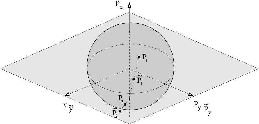
Figure 13: Model II: stereographic projection of $\mathbb{S}^{2}_{x}(h)$ to its equatorial plane with coordinates $(\tilde{y},\tilde{p}_{y})$. The points $\tilde{P}_{1}$ and $\tilde{P}_{2}$ are the images of the points $P_{1}$ and $P_{2}$ under the projection (47).

Points on the hemisphere $B^{2}_{+,x}(h)$ of $\mathbb{S}^{2}_{x}(h)$, which we defined in (37), are projected to the circular disk bounded by the equator (39) (e.g., the point $P_{1}$ in Fig. 13). The North pole is mapped to the center of this disk. Points on the hemisphere $B^{2}_{-,x}(h)$ defined in (38) are projected to points in the plane outside of the disk (see, e.g., the point $P_{2}$ in Fig. 13). The South pole $(p_{x},p_{y},y)=(-\sqrt{(2h+\lambda x^{2})/\lambda},0,0)$ is mapped to infinity. The equator $\mathbb{S}^{1}_{0,x}(h)$ of $\mathbb{S}^{2}_{x}(h)$ (see (39)) is invariant under the projection. Formally this projection is given by

$$\pi_{\text{sg}\,x}:\mathbb{S}^{2}_{x}(h)\to\overline{\mathds{R}}^{2}\,,\quad(p_{x},p_{y},y)\mapsto(\tilde{y},\tilde{p}_{y})\,,$$ (47)

where

$$\tilde{y}=\frac{y\sqrt{(2h+\lambda x^{2})/\lambda}}{\sqrt{(2h+\lambda x^{2})/\lambda}+p_{x}}\,,\quad\tilde{p}_{y}=\frac{p_{y}\sqrt{(2h+\lambda x^{2})/\lambda}}{\sqrt{(2h+\lambda x^{2})/\lambda}+p_{x}}\,,$$ (48)

and $\overline{\mathds{R}}^{2}$ denotes the compactified plane $\mathds{R}^{2}\cup\{\infty\}$. Note that the familiar standard stereographic projection is from a 2-sphere of unit radius to its equatorial plane where the ‘base point’ of the projection is chosen to be the North pole rather than the South pole like in our choice. This explains the scaling factors and signs in (48) which differ from the standard formulae. We use the projection $\pi_{\text{sg}\,x}$ in (47) to define a map of points $(x,y,p_{x},p_{y})$ on the energy surface $\Sigma(h)$ according to

$$F^{\text{II}}:(x,y,p_{x},p_{y})\mapsto(x,\pi_{{\text{sg}}\,x}(p_{x},p_{y},y))=(x,\tilde{y},\tilde{p}_{y})\,.$$ (49)

The map $F^{\text{II}}$ is singular along the North poles of the spheres $\mathbb{S}^{2}_{x}(h)$, $x\in\mathds{R}$, where $y$ and $p_{y}$ are zero, and $p_{x}$ reaches its minimal value for fixed $x$ and $h$. The set of singular points thus is the backward reaction path which is mapped to infinity. As a result the image of $\Sigma(h)$ under $F^{\text{II}}$ is the Cartesian product $\mathds{R}\times\overline{\mathds{R}}^{2}$. Note that the map $F^{\text{II}}$ preserves the symmetry (34), or more precisely, like in Model I, manifolds which are invariant under the $\mathbb{S}^{1}$ symmetry action (34) are rotationally symmetric about the $x$ axis of the image of $F^{\text{II}}$.

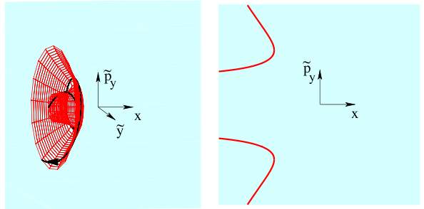
Figure 14: Model II: nonreactive trajectories that stay in the reactants component. The orientation of the $x$, $\tilde{y}$ and $\tilde{p}_{y}$ axes is indicated by the dreibein. The wireframe in the left panel shows a Lagrangian cylinder $\Lambda^{-}_{I,J}$ defined in (14) for $I<0$. The black line shows one of the trajectories contained in $\Lambda^{-}_{I,J}$. The red lines in the right panel show the intersection of $\Lambda^{-}_{I,J}$ with the plane $\tilde{y}=0$.

In the following we use this representation to show geometrical visualizations of the various phase space structures that govern reaction dynamics analogously to Sec. 3.1. Since the energy surface maps to $\mathds{R}\times\overline{\mathds{R}}^{2}$ under $F^{\text{II}}$ we omit a picture of the image of the energy surface. In Fig. 14 we show the $F^{\text{II}}$ image of a Lagrangian manifold $\Lambda^{-}_{I,J}$ with $I<0$ together with a nonreactive trajectory contained in this cylinder. The trajectory comes in from the reactants component ($x\ll-1$) on the left with positive $p_{x}$, spiraling about the $x$ axis. The radius of the rotation increases as $x$ increases. After reaching a maximal $x$ value (where $p_{x}=0$) the trajectory returns deeper and deeper into the reactants region, still spiraling about the $x$ axis with the radius of rotation increasing as $x$ decreases. In Fig. 15 we show the analogous picture for the $F^{\text{II}}$ image of a Lagrangian manifold $\Lambda^{+}_{I,J}$ with $I<0$. The trajectories come in from the products component on the right ($x\gg 1$) with negative $p_{x}$ undergoing rotations with increasing radius about the $x$ axis as $x$ decreases. After reaching a minimal $x$ value, the trajectory returns deeper and deeper into the products region, still undergoing rotation about the $x$ axis, where the radius of the rotation now increases as $x$ increases.

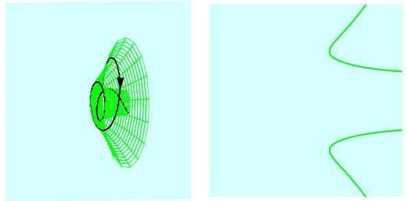
Figure 15: Model II: nonreactive trajectories that stay in the products component. The green wireframe in the left panel shows a Lagrangian cylinder $\Lambda^{+}_{I,J}$ defined in (13) for $I<0$. The black line shows one of the trajectories contained in $\Lambda^{+}_{I,J}$. The green lines in the right panel show the intersection of $\Lambda^{+}_{I,J}$ with the plane $\tilde{y}=0$.

Figure 16 shows the $F^{\text{II}}$ image of a Lagrangian cylinder $\Lambda^{+}_{I,J}$ with $I>0$ together with the forward reaction path which coincides with the $x$ axis. Trajectories contained in $\Lambda^{+}_{I,J}$ evolve from the reactants to the products spiraling about the forward reaction path.

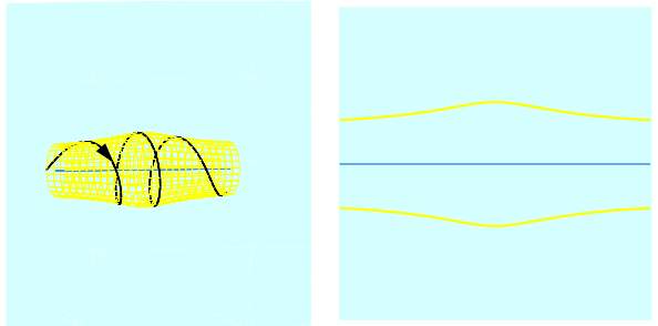
Figure 16: Model II: forward reactive trajectories spiraling about the forward reaction path. The yellow wireframe in the left panel indicates a Lagrangian cylinder $\Lambda^{+}_{I,J}$ with $I>0$. The black line shows a trajectory contained in $\Lambda^{+}_{I,J}$. The blue line shows the forward reaction path. The right panel shows the intersection of $\Lambda^{+}_{I,J}$ with the plane $\tilde{y}=0$ together with the forward reaction path.

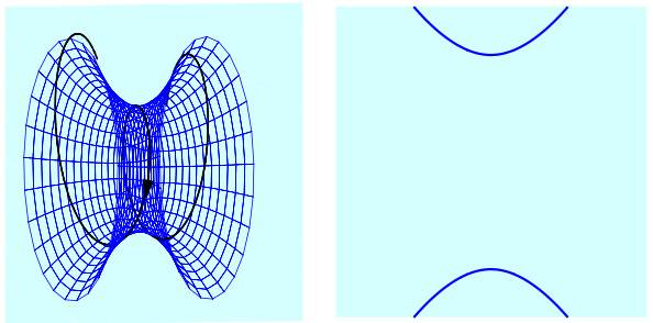
Figure 17: Model II: backward reactive trajectories. The blue wireframe in the left panel indicates a Lagrangian cylinder $\Lambda^{-}_{I,J}$ with $I>0$. The black line shows a trajectory contained in $\Lambda^{-}_{I,J}$. The right panel shows the intersection of $\Lambda^{-}_{I,J}$ with the plane $\tilde{y}=0$.

Figure 17 shows the $F^{\text{II}}$ image of a Lagrangian cylinder $\Lambda^{-}_{I,J}$ with $I>0$ that contains backward reactive trajectories. These trajectories spiral with much larger radii of rotation than the forward reactive trajectories in Fig. 16. In fact, since the backward reaction path is mapped to the line $\mathds{R}\cup\infty$ the backward reactive trajectories can again be considered to spiral about the backward reaction path.

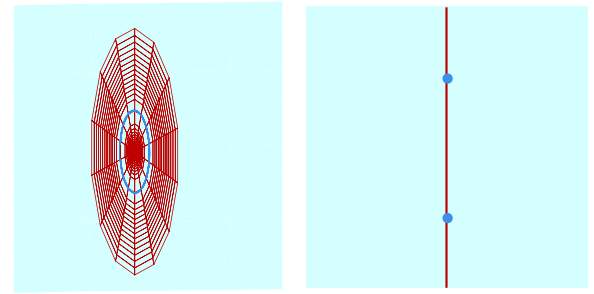
Figure 18: Model II: dividing surface and NHIM. The dark red wireframe in the left panel shows the dividing surface ${\mathbb{S}_{\text{ds}}^{2}(h)}$. The periodic orbit ${\mathbb{S}_{\text{NHIM}}^{1}(h)}$ (blue circle) divides it into the forward hemisphere ${B_{\text{ds,\,f}}^{2}(h)}$ (inner circular disk) and the backward hemisphere ${B_{\text{ds,\,b}}^{2}(h)}$ (outer infinite annulus). The right panel shows the intersection of ${\mathbb{S}_{\text{ds}}^{2}(h)}$ and ${\mathbb{S}_{\text{NHIM}}^{1}(h)}$ with the plane $\tilde{y}=0$.

In Fig. 18 we show the images of the dividing surface ${\mathbb{S}_{\text{ds}}^{2}(h)}$ and the NHIM ${\mathbb{S}_{\text{NHIM}}^{1}(h)}$ under $F^{\text{II}}$. The dividing surface ${\mathbb{S}_{\text{ds}}^{2}(h)}$ maps to the compactified plane $x=0$. The $F^{\text{II}}$ image of the NHIM, ${\mathbb{S}_{\text{NHIM}}^{1}(h)}$, divides it into the forward hemisphere ${B_{\text{ds,\,f}}^{2}(h)}$ which appears as a circular disk in the plane $x=0$ centered about the origin and the backward hemisphere ${B_{\text{ds,\,b}}^{2}(h)}$ which appears as an annulus that extends to the boundary of $\mathds{R}^{2}$ at infinity. The $F^{\text{II}}$ image of the forward reactive trajectories in Fig. 16 which are located near the $x$ axis cross the $F^{\text{II}}$ image of ${B_{\text{ds,\,f}}^{2}(h)}$, and the $F^{\text{II}}$ image of the backward reactive trajectories in Fig. 17 which stay away from the $x$ axis cross the $F^{\text{II}}$ image of ${B_{\text{ds,\,b}}^{2}(h)}$. The two types of trajectories are enclosed by the forward and backward reactive cylinders $W^{s}_{\text{f}}\cup W^{u}_{\text{f}}$ and $W^{s}_{\text{b}}\cup W^{u}_{\text{b}}$ whose $F^{\text{II}}$ images are shown in Figs. 19 and 20, respectively.

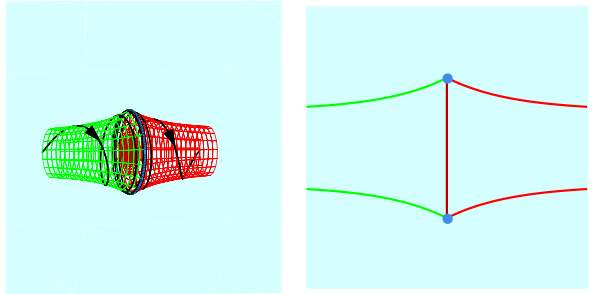
Figure 19: Model II: forward reactive cylinder, forward dividing surface and NHIM. The green and red wireframes in the left panel indicate the branches $W^{s}_{\text{f}}$ and $W^{u}_{\text{f}}$ of the stable resp. unstable manifolds of the NHIM ${\mathbb{S}_{\text{NHIM}}^{1}(h)}$ (blue circle). The black lines show trajectories contained in $W^{s}_{\text{f}}$ and $W^{u}_{\text{f}}$. The dark red wireframe at the center which is difficult to see shows the forward hemisphere ${B_{\text{ds,\,f}}^{2}(h)}$ of the dividing surface. The right panel shows the intersections of the structures on the right with the plane $\tilde{y}=0$.

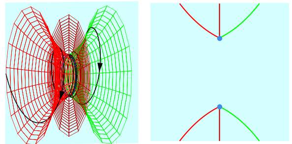
Figure 20: Model II: backward reactive cylinder, backward dividing surface and NHIM. The green and red wireframes in the left panel indicate the branches $W^{s}_{\text{b}}$ and $W^{u}_{\text{b}}$ of the stable resp. unstable manifolds of the NHIM ${\mathbb{S}_{\text{NHIM}}^{1}(h)}$ (blue circle). The black lines show trajectories contained in $W^{s}_{\text{b}}$ and $W^{u}_{\text{b}}$. The dark red wireframe shows the backward hemisphere ${B_{\text{ds,\,b}}^{2}(h)}$ of the dividing surface. The right panel shows the intersections of the structures on the right with the plane $\tilde{y}=0$.

Note that in this geometrical representation of the energy surface (Model II) the bottleneck area of $\Sigma(h)$ associated with the reaction region containing the dividing surface is not so pronounced as in Model I.

3.3 Model III: McGehee representation

The main idea of the third model (Model III) of the energy surface $\Sigma(h)$ is to represent the family of (topological) 2-spheres, $\mathbb{S}^{2}_{x}(h)$, in Eq. (23) parametrized by $x\in\mathds{R}$ as a ‘nested’ set of concentric 2-spheres in $\mathds{R}^{3}$. This can be achieved by projecting each of the 2-spheres, $\mathbb{S}^{2}_{x}(h)$ to a 2-sphere of a radius which depends on $x$. One way to realize this is to map a point $P=(p_{x},p_{y},y)$ on the $\mathbb{S}^{2}_{x}(h)$ according to

$$\pi_{\text{McG}\,x}:(y,p_{x},p_{y})\mapsto(y,p_{x},p_{y})\frac{s(x)}{\lVert(y,p_{x},p_{y})\rVert}=:(\hat{y},\hat{p}_{x},\hat{p}_{y})\,.$$ (50)

Here $\lVert\cdot\rVert$ denotes the Euclidean norm, i.e. $\lVert(p_{x},p_{y},y)\rVert=(p_{x}^{2}+p_{y}^{2}+y^{2})^{1/2}$, and $s$ is the scaling function

$$s(x):=1+\frac{1}{2}\tanh x$$ (51)

which maps the domain $x\in\mathds{R}$ monotonicly to the interval $(1/2,3/2)$. The projection $\pi_{\text{McG}\,x}$ is illustrated in Fig. 21. We name this projection after McGehee who first used this type of construction to present an energy surface of the structure $\mathbb{S}^{2}\times\mathds{R}$ [McGehee(1969)]. A similar construction can also be found in the work by MacKay [MacKay(1990)].

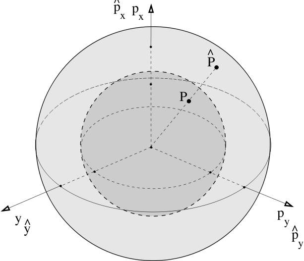
Figure 21: Model III: McGehee projection of a point $P=(y,p_{x},p_{y})$ on the (topological) 2-sphere $\mathbb{S}^{2}_{x}(h)$ (inner dark shaded sphere) to the point $\hat{P}=P=(\hat{y},\hat{p}_{x},\hat{p}_{y})$ on the sphere of radius $s(x)$ (outer light shaded sphere) with $s(x)$ defined in (51). Note that, depending on $x$, the outer sphere could also be inside of the inner sphere, or the two could overlap.

We use $\pi_{\text{McG}\,x}$ in (50) to define a map $F^{\text{III}}$ of points $(x,y,p_{x},p_{y})$ on the energy surface $\Sigma(h)$ to $\mathds{R}^{3}$ according to

$$F^{\text{III}}:(x,y,p_{x},p_{y})\mapsto\pi_{\text{McG}\,x}(p_{x},p_{y},y)=:(\hat{y},\hat{p}_{x},\hat{p}_{y})\,.$$ (52)

Like the maps $F^{\text{I}}$ and $F^{\text{II}}$, the map $F^{\text{III}}$ also preserves the $\mathbb{S}^{1}$ symmetry. In Model III, manifolds that are invariant under the symmetry action (34) have $F^{\text{III}}$ images that are symmetric about the $\hat{p}_{x}$ axis.

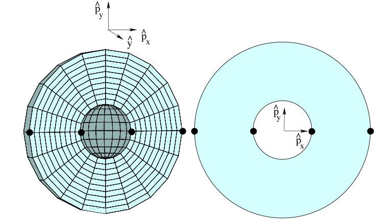
Figure 22: Model III: the energy surface. The left panel shows the energy surface in the threedimensional space with coordinates $(\hat{y},\hat{p}_{y},\hat{p}_{x})$. The orientation of the $\hat{y}$, $\hat{p}_{y}$ and $\hat{p}_{x}$ axes are indicated by the dreibein. (Note that the center of the coordinate system is not the center of the dreibein.) The black points mark the points $(\hat{y},\hat{p}_{y},\hat{p}_{x})=(0,0,\pm 1/2)$ and $(\hat{y},\hat{p}_{y},\hat{p}_{x})=(0,0,\pm 3/2)$ (see text). The right panel shows the intersection of the energy surface with the plane $\hat{y}=0$.

The image of the energy surface $\Sigma(h)$ of topology $\mathds{R}\times\mathbb{S}^{2}$ under the map $F^{\text{III}}$ is the ‘spherical shell’ consisting of the open ball of radius $3/2$ in $\mathds{R}^{3}$ minus the closed ball of radius $1/2$. This image is shown in Fig. 22. The reactants region $x\ll-1$ is contained in the outer region of this spherical shell; the products region $x\gg 1$ is contained in the inner region.

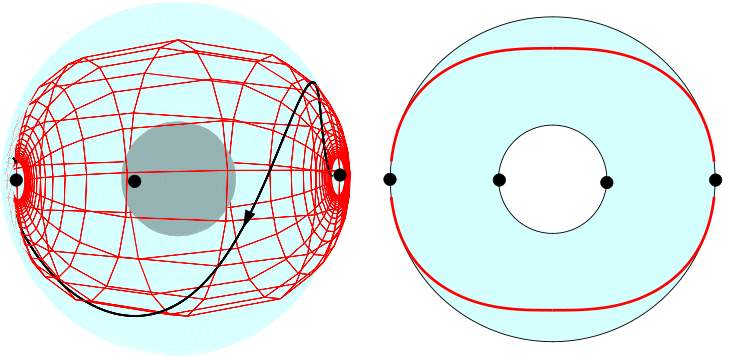
Figure 23: Modell III: nonreactive trajectories that stay in the reactants component. The red wireframe in the left panel indicates a Lagrangian cylinder $\Lambda^{-}_{I,J}$ defined in (14) for $I<0$. The black line shows one of the trajectories contained in $\Lambda^{-}_{I,J}$. The red lines in the right panel show the intersection of $\Lambda^{-}_{I,J}$ with the plane $\hat{y}=0$.

In Fig. 22 we also marked the points $(\hat{y},\hat{p}_{y},\hat{p}_{x})=(0,0,\pm 1/2)$ and $(\hat{y},\hat{p}_{y},\hat{p}_{x})=(0,0,\pm 3/2)$ to which the $F^{\text{III}}$ images of all trajectories converge as time goes to $-\infty$ or $+\infty$ (as long as the trajectory is unbounded in the respective limit). This is a consequence of the conservation of the integrals $I$ and $J$ (the energy in the $x$ and $y$ degrees of freedom, respectively) which implies that $y$ and $p_{y}$ are bounded for each trajectory whereas $p_{x}$ diverges as $x$ goes to $-\infty$ or $+\infty$. In Fig. 23 we show the example of the $F^{\text{III}}$ image of a Lagrangian cylinder $\Lambda^{-}_{I,J}$ defined for $I<0$. The trajectories in $\Lambda^{-}_{I,J}$ come in from deep in the reactants region where $x\ll-1$ and $p_{x}\gg 1$ which is asymptotically (in the limit $t\to-\infty$) mapped to $(\hat{y},\hat{p}_{y},\hat{p}_{x})=(0,0,3/2)$ under $F^{\text{III}}$ and return deep into the reactants region where $x\ll-1$ and $p_{x}\ll-1$ which is asymptotically (in the limit $t\to\infty$) mapped to $(\hat{y},\hat{p}_{y},\hat{p}_{x})=(0,0,-3/2)$ under $F^{\text{III}}$.

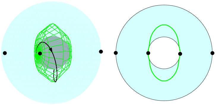
Figure 24: Modell III: nonreactive trajectories that stay in the products component. The green wireframe in the left panel indicates a Lagrangian cylinder $\Lambda^{+}_{I,J}$ defined in (13) for $I<0$. The black line shows one of the trajectories contained in $\Lambda^{+}_{I,J}$. The green lines in the right panel show the intersection of $\Lambda^{+}_{I,J}$ with the plane $\hat{y}=0$.

In Fig. 24 we show the $F^{\text{III}}$ image of a Lagrangian cylinder $\Lambda^{+}_{I,J}$ with $I<0$ which contains nonreactive trajectories in the products region. They come in from deep in the products region $x\gg 1$ with $p_{x}\ll-1$ which under $F^{\text{III}}$ is mapped to $(\hat{y},\hat{p}_{y},\hat{p}_{x})=(0,0,-1/2)$ and move back deep into the products region $x\gg 1$ with $p_{x}\gg 1$ which under $F^{\text{III}}$ is mapped to $(\hat{y},\hat{p}_{y},\hat{p}_{x})=(0,0,1/2)$.

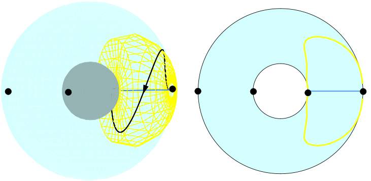
Figure 25: Model III: forward reactive trajectories spiraling about the forward reaction path. The yellow wireframe in the left panel indicates a Lagrangian cylinder $\Lambda^{+}_{I,J}$ with $I>0$. The black line shows a trajectory contained in $\Lambda^{+}_{I,J}$. The blue line shows the forward reaction path. The right panel shows the intersection of $\Lambda^{+}_{I,J}$ with the plane $\hat{y}=0$ together with the forward reaction path.

Fig. 25 shows the $F^{\text{III}}$ image of a Lagrangian cylinder $\Lambda^{+}_{I,J}$ which has $I>0$. The Lagrangian manifold consists of forward reactive trajectories which spiral about the forward reaction path that is also shown in Fig. 25.

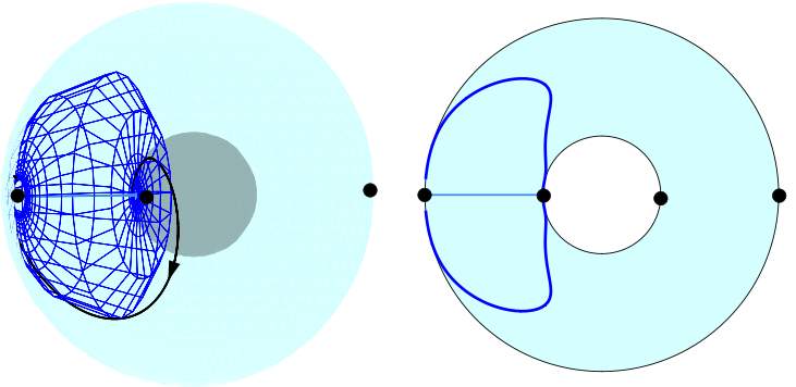
Figure 26: Model III: backward reactive trajectories spiraling about the backward reaction path. The blue wireframe in the left panel indicates a Lagrangian cylinder $\Lambda^{-}_{I,J}$ with $I>0$. The black line shows a trajectory contained in $\Lambda^{-}_{I,J}$ spiraling about the backward reaction path marked in blue. The right panel shows the intersection of $\Lambda^{-}_{I,J}$ with the plane $\hat{y}=0$ together with the backward reaction path.

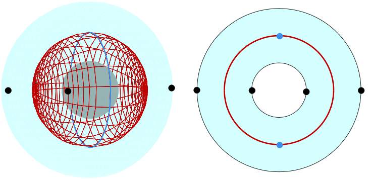
Figure 27: Model III: dividing surface and NHIM. The dark red wireframe in the left panel shows the dividing surface ${\mathbb{S}_{\text{ds}}^{2}(h)}$. The periodic orbit ${\mathbb{S}_{\text{NHIM}}^{1}(h)}$ (blue circle) divides it into the forward hemisphere ${B_{\text{ds,\,f}}^{2}(h)}$ (the hemisphere on the right) and the backward hemisphere ${B_{\text{ds,\,b}}^{2}(h)}$ (the hemisphere on the left). The right panel shows the intersection of ${\mathbb{S}_{\text{ds}}^{2}(h)}$ and ${\mathbb{S}_{\text{NHIM}}^{1}(h)}$ with the plane $\hat{y}=0$.

Fig. 26 shows the analogous image of a Lagrangian cylinder $\Lambda^{-}_{I,J}$ which has $I>0$ and hence consists of backward reactive trajectories.

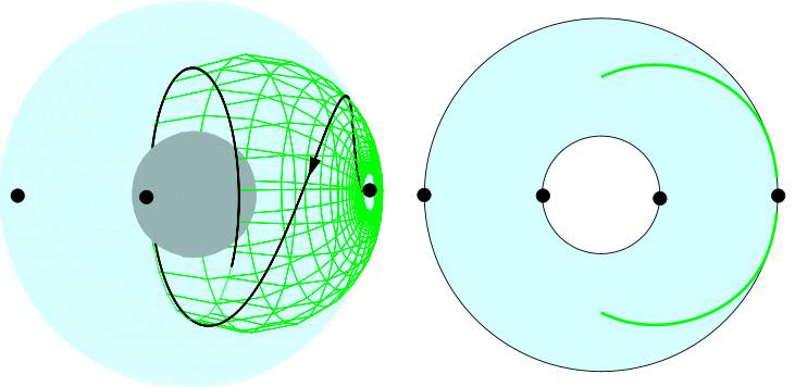
Figure 28: Model III: the forward branch of the stable manifold. The green wireframe in the left panel shows $W^{s}_{\text{f}}$. The black line shows a trajectory contained in $W^{s}_{\text{f}}$. The green lines in the right panels show the intersection of $W^{s}_{\text{f}}$ with the plane $\hat{y}=0$.

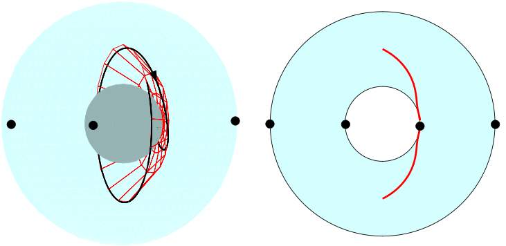
Figure 29: Model III: the forward branch of the unstable manifold. The red wireframe in the left panel shows $W^{u}_{\text{f}}$. The black line shows a trajectory contained in $W^{u}_{\text{f}}$. The red lines in the right panels show the intersection of $W^{u}_{\text{f}}$ with the plane $\hat{y}=0$.

For clarity we show the $F^{\text{III}}$ images of the branches $W^{s}_{\text{f}}$, $W^{u}_{\text{f}}$, $W^{s}_{\text{b}}$ and $W^{u}_{\text{b}}$ of the stable and unstable manifolds of the NHIM separately in Figs. 28-31.

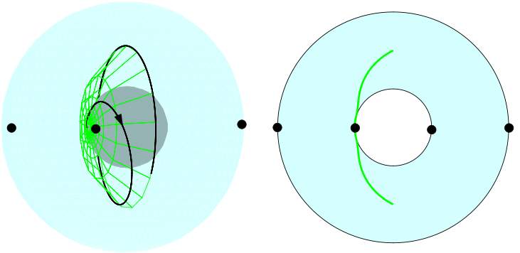
Figure 30: Model III: the backward branch of the stable manifold. The green wireframe in the left panel shows $W^{s}_{\text{b}}$. The black line shows a trajectory contained in $W^{s}_{\text{b}}$. The green lines in the right panels show the intersection of $W^{s}_{\text{b}}$ with the plane $\hat{y}=0$.

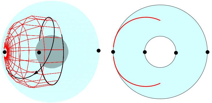
Figure 31: Model III: the backward branch of the unstable manifold. The red wireframe in the left panel shows $W^{u}_{\text{b}}$. The black line shows a trajectory contained in $W^{u}_{\text{b}}$. The red lines in the right panels show the intersection of $W^{u}_{\text{b}}$ with the plane $\hat{y}=0$.

The $F^{\text{III}}$ image of the union $W^{s}_{\text{f}}\cup W^{u}_{\text{f}}$ forms the forward reactive cylinder in Model III. It encloses the $F^{\text{III}}$ image of all forward reactive trajectories as can be seen from comparing Fig. 25 with Fig. 32. Similarly the $F^{\text{III}}$ image of the backward reactive cylinder $W^{s}_{\text{b}}\cup W^{u}_{\text{b}}$ encloses the $F^{\text{III}}$ image of all backward reactive cylinder as can be seen from comparing Fig. 26 with Fig. 33.

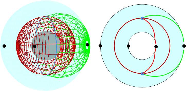
Figure 32: Model III: the forward reactive cylinder, the dividing surface and the NHIM as a superposition of Figs. 27, 28 and 29.

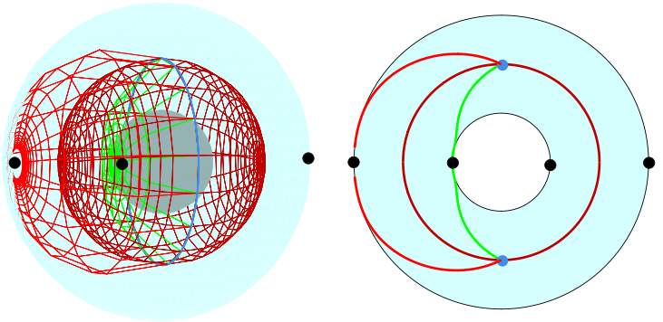
Figure 33: Model III: the backward reactive cylinder, the dividing surface and the NHIM as a superposition of Figs. 27, 30 and 31.

3.4 Implications for Nonlinear Hamiltonian Vector Fields

We have chosen to develop the three models of the phase space structures near a saddle $\times$ centre equilibrium by considering a quadratic, two degree of freedom Hamiltonian which is the normal form, through second order, in the neighborhood of such an equilibrium point. The advantage of this is that is provided very explicit formulae for the phase space structures that allowed straightforward graphical representation. However, precisely the same geometrical structures exist for nonlinear Hamiltonian vector fields in the neighborhood of a saddle $\times$ center equilibrium point. In the nonlinear case the phase space structures can again be described by explicit mathematical formulae using a normal expansion at the saddle $\times$ center equilibrium (see Sec. 2.2, and [Waalkens et al.(2008)] for a detailed discussion). For a given system, this in general leads a Hamilton function which is a power series rather than a linear function of the integrals $I$ and $J$ (see (20)). The coefficients of this powers series are obtained from the normal form calculations for an explicit systems.

Nevertheless, the normal form theory allows us to conclude that the same geometrical structures, having the same interpretation and meaning, hold for more general, nonlinear Hamiltonian vector fields in the neighborhood of a saddle center-$\ldots$-center equilibrium point, but obtaining the explicit formulae will require a normal form calculation for a given system. It is in this sense that restricting ourselves to quadratic Hamiltonians is, indeed, ”without loss of generality”, and it provides the method and approach for visualizing the same phase space structures governing reaction dynamics in more general systems.

4 A model of the $n$-DoF system in the space of the integrals of motion

For a system with more than 2 degrees of freedom, the dimensionality of the phase space structures discussed in Sec. 2 is too high to allow for a similar explicit visualization like for the 2-DoFmodels in Sec. 3. Instead of projecting the phase space structures to the planes of the coordinates and conjugate momenta of the normal form like in Sec. 2.2 it is useful to present the phase space structures for $n$ DoFin the space of the integrals $I,J_{2},\ldots,J_{n}$. This can be accomplished using the momentum map ${\cal M}$ defined in (12) in Sec. 2.3. The discussion here follows [Waalkens et al.(2008)].

As mentioned in Sec. 2.3 a fibre (the joint level set of the integrals $I,J_{2},\ldots,J_{n}$ in phase space) is called singular if it contains one (or more) irregular point(s). The image of all the singular fibres under the momentum map is called the bifurcation diagram. It is easy to see that the bifurcation diagram consists of the set of $(I,J_{2},\ldots,J_{n})$, where one or more of the integrals vanish. In Fig. 34 we show the image of the energy surface with energy $h>0$ under the momentum map ${\cal M}$ in the space of the integrals for $n=3$ degrees of freedom.

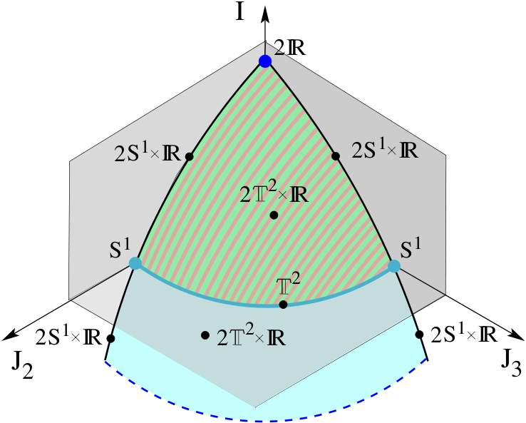
Figure 34: Sketch of the image of the energy surface of energy $h>0$ under the momentum map ${\cal M}$ in Equation (12) in the space of the integrals $I$ and $J_{k}$, $k=2,\ldots,n$, for the case of $n=3$ degrees of freedom. The green/dark pink brindled piece of the image of the energy surface has $I>0$; the turquoise piece has $I<0$. The intersections with the planes $I=0$, $J_{2}=0$ and $J_{3}=0$ (pieces of which are visualised by semitransparent planes for clarity) form the bifurcation diagram of the energy surface. The image of the energy surface is not bounded in the direction of negative $I$ as indicated by the dashed line at the bottom. The topology of the fibres ${\cal M}^{-1}(I,J_{2},J_{3})$ is indicated for the various points $(I,J_{2},J_{3})$ marked by dots. The fibre of a point $(I,J_{2},J_{3})$ with $I\neq 0$ consists of two disconnected manifolds as indicated by the factor of 2. The fibre of a point $(I,J_{2},J_{3})$ with $I=0$ consists of a single connected manifold.

The bifurcation diagram (of the energy surface) consists of the intersections of the image of the energy surface (the turquoise and green/dark ping brindled surface in Fig. 34) with one of the planes $I=0$, $J_{2}=0$ or $J_{3}=0$. Upon approaching one of the edges that have $J_{2}=0$ or $J_{3}=0$ the circle in the plane $(q_{2},p_{2})$ or $(q_{3},p_{3})$, respectively, shrinks to a point, and accordingly the regular fibres $\mathds{T}^{2}\times\mathds{R}$ which form the Lagrange manifolds $\Lambda^{+}_{I,J_{2},\ldots,J_{n}}$ and $\Lambda^{-}_{I,J_{2},\ldots,J_{n}}$ (see (13) and (14)) reduce to cylinders or ‘tubes’ $\mathbb{S}^{1}\times\mathds{R}$. At the top corner in Fig. 34 both $J_{2}$ and $J_{3}$ are zero. Here both circles in the centre planes $(q_{2},p_{2})$ and $(q_{3},p_{3})$ have shrinked to points. The corresponding singular fibre consists of two lines, $\mathds{R}$, which are the forward and backward reaction paths, respectively (see also Fig. 4).

The fibres mentioned so far all have $I\neq 0$ and each consist of a pair of two disconnected components. For $I<0$, one member of each pair is located on the reactants side and the other on the products side of the dividing surface. For $I>0$, one member of each pair consists of trajectories evolving from reactants to products and the other member consists of trajectories that evolve from products to reactants. In fact the two members of a fibre which has $I>0$ are contained in the energy surface volume enclosed by the forward and backward reactive spherical cylinders $W_{f}(h)$ and $W_{b}(h)$, see Fig. 4. For this reason we marked the piece of the image of the energy surface under the momentum map which has $I>0$ by the same green/dark pink colour in Fig. 34 that we used Fig. 4. Green corresponds to forward reactive trajectories and dark pink corresponds to backward reactive trajectories. Under the momentum map these trajectories have the same image.

The light blue line in Fig. 34 which has $I=0$ is the image of the NHIM under the momentum map. For three degrees of freedom, the NHIM is a 3-dimensional sphere, and as we will discuss in more detail in Sec. 5 and indicated in Fig. 34 it is foliated by a one-parameter family of invariant 2-tori which shrink to periodic orbits, i.e. circles, $\mathbb{S}^{1}$, at the end points of the parameterisation interval.

5 Structure of the NHIM for $n$-DoF

We have described how the NHIM, its stable and unstable manifolds, and the dividing surface, sit within the phase space and govern the reaction dynamics in several 2DoF geometrical models. However, we have not given any indication of the structure of the NHIM itself, except in the $2$-DoF case, in which the NHIM is a single periodic orbit. In this section we discuss various ways of visualizing the geometrical structure and dynamics associated with the NHIM.

Recall from Sec. 2.2 that in terms of the local decoupling provided by the normal form into reaction coordinates and bath modes, points on the NHIM, ${\mathbb{S}_{\text{NHIM}}^{2n-3}(h)}$, contain zero ‘energy’ in the reactive (saddle) mode (i.e., $I=0$); all ‘energy’ is contained in the bath (centre) modes, which results in oscillatory, quasiperiodic motion with $n-1$ independent frequencies. As also mentioned in Sec. 2.2, this leads to the interpretation of the NHIM as the energy surface of an invariant subsystem with one degree of freedom less than the full system (a supermolecule located for a frozen reaction coordinate (and conjugate momentum) between reactants and products).

Since, typically (for more than $1$ DoF), there is more than one bath mode present, the total energy can be distributed in a variety of ways amongst the bath modes. For example, putting all of the energy into any one of the bath modes results in a single periodic orbit (often referred to as a Lyapunov orbit). More generally, the supermolecule of fixed energy $h$ has energy distributed between all of the $n-1$ bath modes. Since the integrals of motion are constant on trajectories, the amount of energy in each particular bath mode remains fixed during the motion. Such a molecule therefore undergoes quasiperiodic motion; it oscillates independently in the $n-1$ different bath modes. The motion of a typical trajectory in the NHIM is quasiperiodic on an $(n-1)$-torus. Heuristically, one can think of the NHIM as the invariant surface made up of trajectories with all possible energy distributions between the bath modes (and no energy in the reactive mode).

5.1 The NHIM $\mathbb{S}^{3}$ ($n=3$ DoF)

As noted above, the NHIM for $2$-DoF systems is simply a periodic orbit. This is an immediate consequence of the fact that there is only a single bath (or centre) mode. In this section we consider the next most complex case in some detail, the $3$-DoF situation ($2$ bath modes), for which the NHIM is diffeomorphic to $\mathbb{S}^{3}$. However, first we will describe a way in which $\mathbb{S}^{3}$ can be visualized in lower dimensions. This is helpful from the point of view of visual intuition. Our discussion in this section owes a great deal to the nice report of [Chisholm(2000)].

Geometrical Construction of $\mathbb{S}^{3}$ in Three Dimensions.

To begin with, first note that in the usual manner, to draw a 1-sphere (i.e. a circle), we need two dimensons, to draw a 2-sphere we need three dimensions, and to draw a 3-sphere we need four dimensions. We will describe a method of drawing the 3-sphere which requires only three dimensions. This particular representation will enable us to make a clear picture of the dynamics on the NHIM. The method can be viewed as a generalization of the presentation of a two-dimensional sphere, $\mathbb{S}^{2}$, in terms of two hemispheres (topological 2–balls, $B^{2}$) and an equator (a onedimensional sphere, $\mathbb{S}^{1}$) that we discussed in Sec. 3.1. For $\mathbb{S}^{3}$, one can form a similar representation by using two open $3$-balls, $B^{3}$, to represent “Northern” and “Southern” hemispheres, and identifying points on their boundaries, $\mathbb{S}^{2}$, to make an “equator”;

$$\mathbb{S}^{3}\equiv B^{3}_{\text{North}}\cup\mathbb{S}^{2}_{\text{Equator}}\cup B^{3}_{\text{South}}.$$ (53)

We will choose the “North” pole (N) to be at the centre of the North ball and the “South” (S) pole at the centre of the South ball. This model is illustrated in Fig. 35.

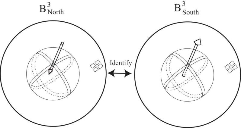
Figure 35: A model of the sphere $\mathbb{S}^{3}$ formed by taking two open $3$-balls, $B^{3}_{\text{North}}$ and $B^{3}_{\text{South}}$, and identifying points on their boundaries; the “equator” $\mathbb{S}^{2}_{\text{Equator}}$. The arrow in $\mathbb{S}^{3}$ illustrates how one passes from the chosen “North” to the chosen “South” pole at the center of each $3$-ball.

Partitioning ‘Energy’ Between the Two Bath Modes

Recall that (for $3$ DoF) there are $2$ bath modes. For a given trajectory in the NHIM, all of the ‘energy’ could be in the first bath mode (resulting in a periodic orbit) or in the second bath mode (resulting in another periodic orbit), or the energy could be distributed, or partitioned, between the two bath modes.

In Fig. 36(a) we show the two open balls that comprise our model of $\mathbb{S}^{3}$ as described above. We choose a trajectory having the property that all of the energy is in the first bath mode, i.e., $J_{3}=0$ and $J_{2}=J_{2}^{\text{max}}$, where $J_{2}^{\text{max}}$ is defined by the energy equation, $K_{\text{NF}}(0,J_{2}^{\text{max}},0)=h>0$ (see Sec. 2.2). This corresponds to a periodic orbit that moves along the “vertical” circle that passes through the centers of the two balls. As the periodic orbit exits the North ball at the top, it enters the South ball from the top, exiting the South ball at the bottom, and entering the North ball at the bottom.

Suppose now that we change this distribution of energy very slightly, by taking a small amount of energy out of the first bath mode and putting it into the second, which we illustrate in Fig. 36(b) (and where we leave it to the reader to consider how a trajectory leaves one ball through its surface and enters the other ball). The motion still stays close to the original circle, but there is now a second circular (oscillatory) motion “around the periodic orbit”. Thus the motion now takes place on a thin $2$-torus. Any initial condition on the $2$-torus corresponds to a quasiperiodic trajectory that remains on the $2$-torus.

We continue this procedure of taking energy from the first bath mode and putting it into the second bath mode, until all of the energy is in the second bath mode (Fig. 36(e)), which results in a periodic orbit moving in a “horizontal” circle along the surface of the two balls.

$B^{3}_{\text{North}}$	$B^{3}_{\text{South}}$

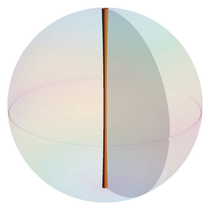
(a)

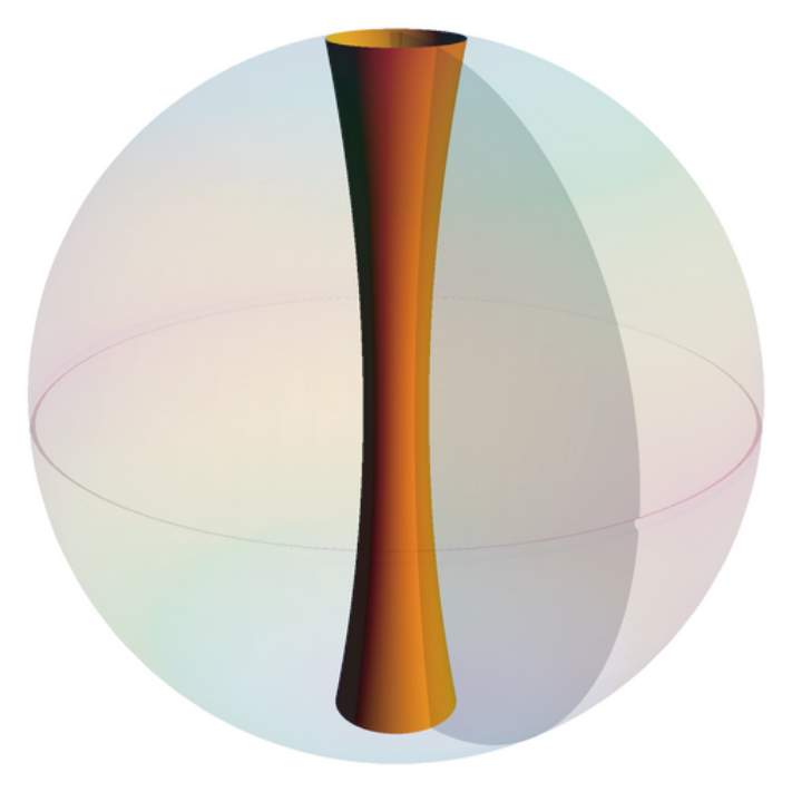
(b)

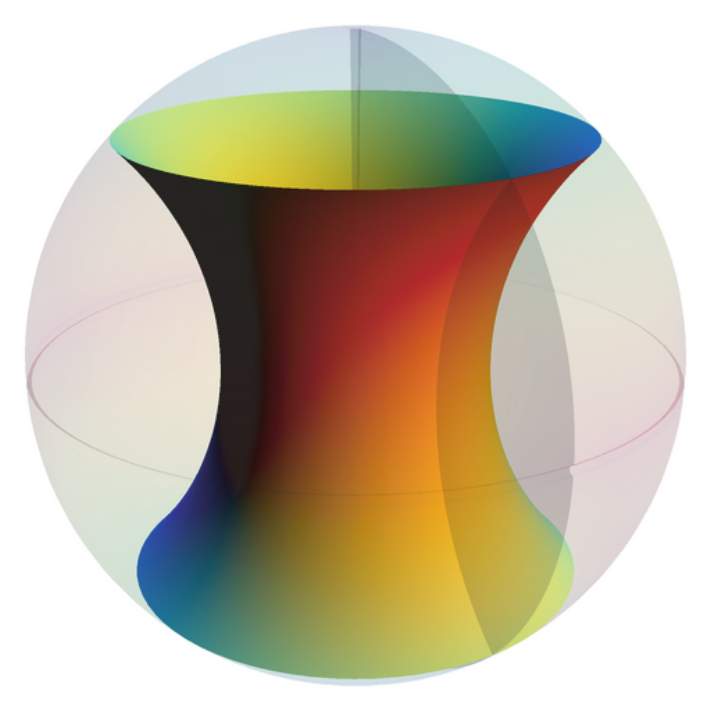
(c)

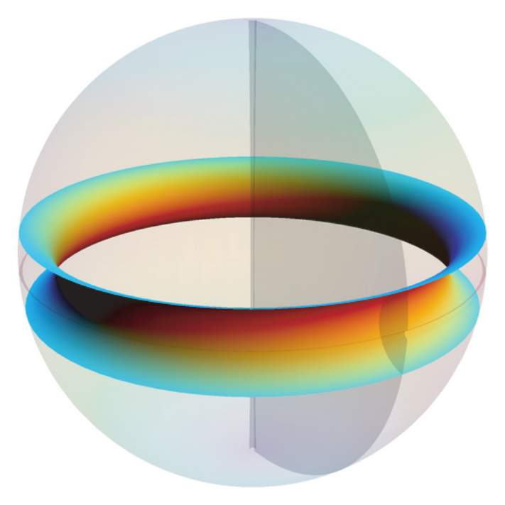
(d)

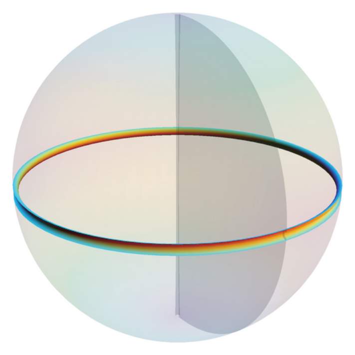
(e)

Figure 36: Illustration of the invariant tori in ${\mathbb{S}_{\text{NHIM}}^{2n-3}(h)}$, for $n=3$ degrees of freedom. (a) representation of the periodic orbit corresponding to local integrals of motion $(I,J_{2},J_{3})=(0,J_{2}^{\text{max}},0)$, shown in both hemispheres of the model, (b) a nearby torus with $J_{3}=\epsilon$ with $0<\epsilon\ll J_{2}^{\text{max}}$, (c) the case $J_{2}=J_{2}^{\text{max}}/2$, (d) a torus with $J_{3}=J_{3}^{\text{max}}-\epsilon$ which is close to the periodic orbit corresponding to $(I,J_{2},J_{3})=(0,0,J_{3}^{\text{max}})$, shown in (e).

In this way we see that $\mathbb{S}^{3}$ is foliated by a one-parameter family of 2-tori. Trajectories on the 2-tori correspond to quasiperiodic motion with energy contained in both bath modes. The “extreme” cases corresponding to all the energy contained in one of the bath modes corresponds to periodic orbits (the “Lyapunov orbits”). We illustrate this family of 2-tori in Fig. 37.

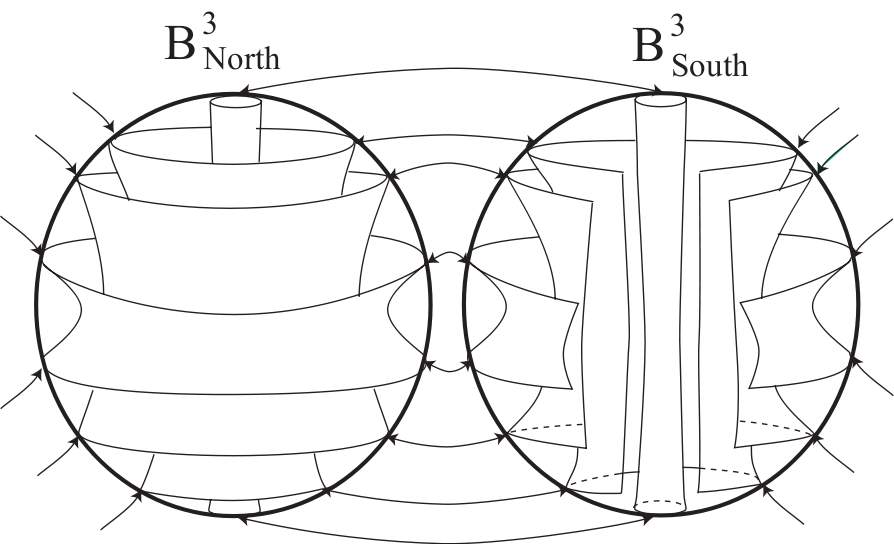
$\leftarrow$ Identify $\rightarrow$

Figure 37: The family of invariant $2$-tori that fill the NHIM, $\mathbb{S}^{3}_{\text{NHIM}}$, illustrated according to our method for visualizing $\mathbb{S}^{3}$ in three dimensions. One can think of each torus as being cut in half, with one half in the North ball and the other half in the South ball, and the “edges” of the two halves touching touching the surface of the $3$-ball, where they are identified. In this way, a quasiperiodic trajectory winding around a $2$-torus continually moves from one $3$-ball to another as it encounters the edge of the torus where the torus is cut into two pieces, which are on the surfaces of the $3$-balls (i.e. the “equator” of $\mathbb{S}^{3}_{\text{NHIM}}$).

5.2 The NHIM, ${\mathbb{S}_{\text{NHIM}}^{2n-3}(h)}$, for $n>3$ DoF

The method for visualizing the NHIM for 3 DoF described in the previous section is not as useful for $n>3$ DoF. Nevertheless, the dynamics on the NHIM have the same characteristics–quasiperiodic trajectories with the energy partitioned amongst the $n-1$ bath modes. Hence, as mentioned in Sec. 4, for the general DoF case, a description of the NHIM can be given in terms of the geoemtry of the space of centre actions (or “bath mode” actions) $J_{2},\ldots,J_{n}$. This is what we will now describe.

Classically, the space formed by the centre actions is the $(n-1)$-dimensional positive cone; equivalently, the positive orthant (the generalization of a quadrant in the plane or an octant in three dimensions to arbitrary dimensions) given by $J_{2},\ldots,J_{n}\geq 0$ in $\mathbb{R}^{n-1}$. In general, the NHIM is represented in this space by a (topological) $(n-2)$-simplex having $(n-1)$ vertices, one for each centre action. The vertices are always located on the coordinate axes; each vertex thus corresponds to $(n-2)$ of the integrals $J_{k}$ being equal to zero. Note that the projection of the NHIM to this space of actions will generally be a nonlinear embedding of a simplex; the embedding is only linear (that is, all cells of the simplex are flat) in the case where the vector field defined by Hamilton’s equations is linear. We will denote this embedded simplex by

$$\Lambda=[2,3,\ldots,n],$$ (54)

using the index of each centre action to label a vertex. Within this simplex, each $(k-1)$-cell (for every $k=1,\ldots,(n-1)$), denoted $[j_{1},\ldots,j_{k}]$, represents a $(k-1)$-parameter family of invariant $k$-tori which we denote by

$$\mathbb{T}^{k}_{j_{1}j_{2}\ldots j_{k}}.$$ (55)

Here $j_{1},,\ldots,j_{k}$ are mutually different elements of $\{2,\ldots,n\}$ which indicate the center actions $J_{j_{1}},\ldots,J_{j_{k}}$ are different from zero. The family is parameterised, for example, by the centre actions $J_{j_{1}},\ldots,J_{j_{k-1}}$, with the value of $J_{j_{k}}$ being determined by the energy equation, as we will describe below.

For example, each vertex (i.e., $0$-cell), denoted $[j]$ (for $j=2,\ldots,n$), represents a single periodic orbit $\mathbb{T}^{1}_{j}\cong\mathbb{S}^{1}$, in which all actions except $J_{j}$ are set to zero and, therefore, the remaining action is fixed at a value $J_{j}=J_{j}^{\text{max}}$, which solves the following equation that corresponds to restriction to a single energy surface,

$$K_{\text{NF}}(I,J_{2},\ldots,J_{n})=h>0,$$ (56)

subject to setting ${J_{\ell}}=0$ for all $\ell=2,\ldots,n$, $\ell\neq j$. The periodic orbit, $\mathbb{T}^{1}_{j}$, projects to a single circle of radius $\sqrt{J_{k}^{\text{max}}}$ in the $(q_{k},p_{k})$-plane of the normal form coordinates and to the origin in all other normal form planes, $(q_{\ell},p_{\ell})$ for $\ell\neq j$.

Each edge $[j_{1},j_{2}]$ (for $j_{1}\neq j_{2}$) of the simplex represents a $1$-parameter family of invariant $2$-tori, in which all actions except $J_{j_{1}}$ and $J_{j_{2}}$ have been set to zero. Without loss of generality, we can choose $J_{j_{1}}$ as a parameter; each value $J_{j_{1}}\in[0,J_{j_{1}}^{\text{max}}]$ fixes the value of $J_{j_{2}}$ by virtue of the above iso-energetic condition subject to the modified restriction that

$$J_{\ell}=0\ \mbox{for $\ell\neq j_{1},j_{2}$}.$$ (57)

We denote this $1$-parameter family of invariant $2$-tori in ${\mathbb{S}_{\text{NHIM}}^{2n-3}(h)}$ by $\mathbb{T}^{2}_{j_{1}j_{2}}$.

By allowing $k$ centre actions to be non-zero in the NHIM, corresponding to a $(k-1)$-cell $[j_{1},j_{2}\ldots,j_{k}]$ of the simplex, we can, without loss of generality, take $J_{j_{1}},J_{j_{2}},\ldots,J_{j_{k-1}}$ as parameters which fix the value of $J_{j_{k}}$ via the condition

$$H_{\text{NF}}(I,J_{2},\ldots,J_{n})=h>0,$$ (58)

subject to setting

$${J_{\ell}=0\ \mbox{for $\ell\neq j_{1},j_{2},\ldots,j_{k}$.}}$$ (59)

This defines a $(k-1)$-parameter family of invariant $k$-tori, denoted $\mathbb{T}^{k}_{j_{1}j_{2}\ldots j_{k}}$.

A schematic representation of the projection of ${\mathbb{S}_{\text{NHIM}}^{2n-3}(h)}$ into the space of centre actions $J_{2},J_{3},\ldots,J_{n}$ for $n$-DoF is shown in Fig. 38 for (i) $n=3$, (ii) $n=4$, (iii) $n=5$. In (iii) we show a schematic $3$-dimensional projection of the $4$-dimensional space of centre actions.

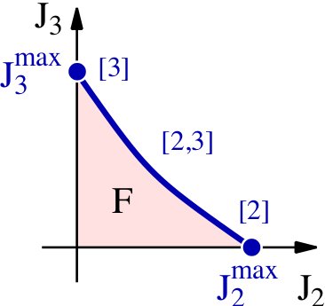
(i) $n=3$ degrees of freedom.

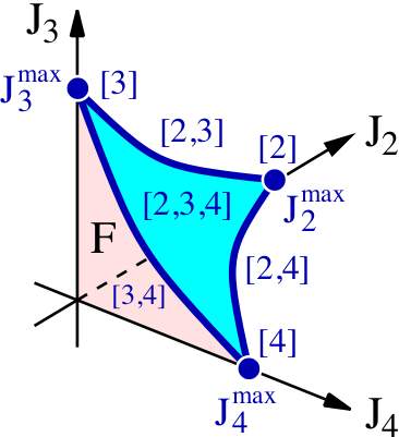
(ii) $n=4$ degrees of freedom.

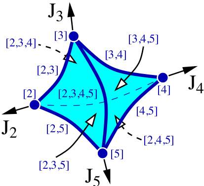
(iii) $n=5$ degrees of freedom.

Figure 38: Schematic representation of the projection of ${\mathbb{S}_{\text{NHIM}}^{2n-3}(h)}$ into the space of centre actions, $J_{2},J_{3},\ldots,J_{n}$, for $n$ DoF giving a nonlinear embedding of a simplex with $(n-1)$ vertices, $[j]$, $j=2,\ldots,n$, which encloses a volume proportional to the directional flux, $F$.

Directional flux across the dividing surface.

In [Waalkens & Wiggins(2004)] it is shown that the (directional) flux across a given iso-energetic dividing surface ${\mathbb{S}_{\text{ds}}^{2n-2}(h)}$ (that is, the equal and opposite fluxes through the forward and backward dividing surface hemispheres ${B_{\text{ds,\,f}}^{2n-2}(h)}$ and ${B_{\text{ds,\,b}}^{2n-2}(h)}$) may be reduced to a certain integral taken over ${\mathbb{S}_{\text{NHIM}}^{2n-3}(h)}$. In the representation of the NHIM in in terms of the centre integrals given above, this flux corresponds to the $(n-1)$-dimensional volume of the finite region of the positive orthant bounded by the $(n-2)$-simplex representing the NHIM times $(2\pi)^{n-1}$. That is up to a factor, the flux corresponds to the volume of an $(n-1)$-simplex formed by adding the origin to the vertex set of the NHIM in the space of integrals. In Fig. 38 for (i) and (ii), the $(n-1)$-dimensional volume $F$ corresponding to the magnitude of the directional flux across the dividing surface hemispheres ${B_{\text{ds,\,f}}^{2n-2}(h)}$ and ${B_{\text{ds,\,b}}^{2n-2}(h)}$ is indicated. Applications of this in both the classical and quantum case can be found in [Waalkens et al.(2008)].

6 Conclusions

This paper is concerned with strategies and approaches for visualizing the phase space structures that govern reaction dynamics. In Section 2 we reviewed recent results that develop the phase space geometry near an equilibrium point of Hamilton’s equations of $\mbox{saddle}\times\mbox{centre}\times\cdots\times\mbox{centre}$ stability type (‘saddle’ for short) in $n$ degree-of-freedom Hamiltonian systems. The key technique used was the method of Poincaré-Birkhoff normal forms. This method provided a transformation (and its inverse), valid in a phase space neighborhood of the equilibrium point, to normal form coordinates in which the phase space structures could be explicitly realized (and then mapped back to the original coordinates via the inverse of the normal form transformation). The key phase space structure was seen to be a normally hyperbolic invariant manifold (NHIM), which is the higher dimensional analogue of a “saddle point”. The NHIM is the anchor upon which a dividing surface having the “no-recrossing” property and minimal flux is constructed. Moreover, the stable and unstable manifolds of the NHIM are the “conduits” for forward and backward reactive trajectories (trajectories evolving from reactants to products, and vice-versa). More precisely, one the two branches of the stable manifold can be glued together with one of the two branches of the unstable manifold to form a cylinder (denoted the forward reactive cylinder in this paper) that enclose all forward reactive trajectories; and the other branches of the stable and unstable manifolds can be glued together to form a cylinder (the backward reactive cylinder) which encloses all backward reactive trajectories. In the case where a generic non-resonance condition holds on the pure imaginary eigenvalues associated with the center directions it follows that in the normal form coordinates the Hamiltonian (when the series representing the normal form Hamiltonian is truncated at some finite order) has $n$ integrals of the motion and thus is integrable. This integrable structure allows for a natural decoupling of the dynamics into a single reactive mode and $n-1$ bath modes. Moreover, the integrable structure provides a foliation of the NHIM by a family of lower dimensional tori and a foliation of a neighborhood of the equilibrium point into Lagrangian cylinders.

The “decoupling” of the vector field and the associated dynamics masks the complete picture of reaction governed by the phase space structures in the energy surface. In Section 3 we provide three different 2 degree-of-freedom models that allow us to visualize the energy surface, the NHIM and its stable and unstable manifolds, the dividing surface, and the Lagrangian cylinders. These give a complete picture of how the phase space structures govern the dynamics of trajectories near a saddle. By contrast, the role of the phase space structures is typically obscured in their common representation as projections to configuration. For example, the projection of the volume enclosed by the forward and backward cylinders might not lie inside of the projection of the forward and backward cylinders, and as a consequence forward and backward reactive trajectories might seemingly leave the forward and backward reactive cylinders (for an example, see the study of the planar Hill problem in [Waalkens et al.(2005b)]).

For the general case of $n>2$ degrees of freedom systems, we use the integrals alone to provide a model for visualizing the phase space structures (see Section 4 ). This model does not contain explicit information on trajectories, but it can be easily related to the behavior of trajectories by utilizing the foliation of the neighborhood of the NHIM by Lagrangian cylinders.

We moreover discussed in some detail the foliation of the NHIM for 3 degrees of freedom. Here the NHIM is a threedimensional sphere, $\mathbb{S}^{3}$ that is foliated by a one-parameter family of invariant 2-tori. We visualized this foliation using the 3-ball model of $\mathbb{S}^{3}$ (see Section 5). For the general case of $n>3$ degrees of freedom, we presented the NHIM as a simplex in the space of the integrals. This is of particular importance, since, up to a prefactor, the volume enclosed by the simplex in the positive orthant of the integral space gives the directional flux.

We conclude by emphasizing that we focused the discussion of the phase space structures and their visualization to the neighborhood of the saddle. In fact, depending on the global topology of the energy surface, the local partitioning of the energy surface by the dividing surface constructed from the NHIM into a reactants and a products component might not extend to a global partitioning. For example, there could be more than one saddle point which controls the access to and escape from a certain phase space region which requires a more careful definition of a reactants and a products region. Moreover, in this paper we did not discuss the global geometry of the stable and unstable manifolds of the NHIM. In fact the stable and unstable manifolds might extend to regions far away from the neighborhood of the saddle. Even if there is only a single saddle point, the global structure might be very complicated since the stable and unstable manifolds might wrap around in a complicated manner and intersect each other to form a highdimensional homoclinic tangle. If there are several saddles the stable and unstable manifolds of NHIMs of different saddles might intersect. Since the stable and unstable manifolds are of codimension 1 in the energy surface they still act as impenetrable barriers globally, and also control the global dynamics in a possibly complicated way. The details of the dynamics then strongly depends on the system under consideration. For a few examples, we refer to [Waalkens et al.(2004a), Waalkens et al.(2004b), Waalkens et al.(2005a), Waalkens et al.(2005b), Waalkens et al.(2005c)].

7 Acknowledgements

SW acknowledges the support of the Office of Naval Research Grant No. N00014-01-1-0769, and the stimulating environment of the NSF sponsored Institute for Mathematics and its Applications (IMA) at the University of Minnesota, where this manuscript was completed. HW acknowledges support by EPSRC under Grant No. EP/E024629/1. We are grateful to Dr. Andrew Burbanks for helping with an early version of this manuscript.

References

- [Arnold(1978)] Arnold, V. I. (1978). Mathematical Methods of Classical Mechanics, volume 60 of Graduate Texts in Mathematics. Springer, New York, Heidelberg, Berlin.
- [Arnol’d et al.(1988)] Arnol’d, V. I., Kozlov, V. V., & Neishtadt, A. I. (1988). Mathematical aspects of classical and celestial mechanics. In V. I. Arnol’d, editor, Dynamical Systems III, volume 3 of Encyclopaedia of Mathematical Sciences. Springer, Berlin.
- [Child & Pollak(1980)] Child, M. S. & Pollak, E. (1980). Analytical reaction dynamics: Origin and implications of trapped periodic orbits. J. Chem. Phys., 73(9), 4365–4372.
- [Chisholm(2000)] Chisholm, M. (2000). The sphere in three dimensions and higher: Generalizations and special cases. Available at http://www.theory.org/geotopo/.
- [de Oliveira et al.(2002)] de Oliveira, H. P., Ozorio de Almeida, A. M., Soares, I., & Tonini, E. V. (2002). Homoclinic chaos in the dynamics of a general Bianchi type-IX model. Phys. Rev. D., 65, 083511.
- [Deprit(1969)] Deprit, A. (1969). Canonical transformations depending on a small parameter. Celestial Mech., 1, 12–30.
- [Dragt & Finn(1976)] Dragt, A. & Finn, J. (1976). Lie series and invariant functions for analytic symplectic maps. J. Math. Phys., 17(12), 2215–2227.
- [Eckhardt(1995)] Eckhardt, B. (1995). Transition state theory for ballistic electron transport. J. Phys. A, 28, 3469.
- [Garrett(2000)] Garrett, B. C. (2000). Perspective on “The transition state method,” Wigner E. (1938) Trans. Faraday Soc. 34:29-41. Theor. Chem. Acc., 103, 200–204.
- [Guillemin(1994)] Guillemin, V. (1994). Moment Maps and Combinatorial Invariants of Hamiltonian -spaces. Birkhäuser, Boston.
- [Jacucci et al.(1984)] Jacucci, G., Toller, M., DeLorenzi, G., & Flynn, C. P. (1984). Rate theory, return jump catastrophes, and the center manifold. Phys. Rev. Lett., 52(4), 295–298.
- [Jaffé et al.(2000)] Jaffé, C., Farrelly, D., & Uzer, T. (2000). Transition state theory without time-reversal symmetry: Chaotic ionization of the hydrogen atom. Phys. Rev. Lett., 84, 610–613.
- [Jaffé et al.(2002)] Jaffé, C., Ross, S. D., Lo, M. W., Marsden, J., Farrelly, D., & Uzer, T. (2002). Statistical theory of asteroid escape rates. Phys. Rev. Lett., 89(1), 011101.
- [Komatsuzaki & Berry(1999)] Komatsuzaki, T. & Berry, R. S. (1999). Regularity in chaotic reaction paths. I. Ar-6. J. Chem. Phys., 110(18), 9160–9173.
- [Laidler & King(1983)] Laidler, K. J. & King, M. C. (1983). The development of transition state theory. J. Phys. Chem., 87, 2657–2664.
- [MacKay(1990)] MacKay, R. S. (1990). Flux over a saddle. Phys. Lett. A, 145, 425–427.
- [Mahan(1974)] Mahan, B. H. (1974). Activated complex theory of bimolecular reactions. J. Chem. Edu., 51(11), 709–711.
- [Marsden & Ratiu(1999)] Marsden, J. E. & Ratiu, T. S. (1999). Introduction to Mechanics and Symmetry (2nd edition). Springer-Verlag, Berlin, Heidelberg, New York.
- [McGehee(1969)] McGehee, R. P. (1969). Some Homoclinic Orbits for the Restricted Three-Body Problem. Ph.d. thesis, University of Wisconsin.
- [Meyer(1974)] Meyer, K. (1974). Normal forms for hamiltonian systems. Celestial Mech., 9, 517–522.
- [Meyer(1991)] Meyer, K. (1991). A lie transform tutorial ii. In K. Meyer and D. Schmidt, editors, Computer Aided Proofs in Analysis, volume 28 of The IMA Volumes in Mathematics and its Applications, pages 190–210, New York, Heidelberg, Berlin. Springer-Verlag.
- [Meyer & Hall(1992)] Meyer, K. & Hall, G. (1992). Introduction to Hamiltonian Dynamical Systems and the N-Body Problem, volume 90 of Applied Mathematical Sciences. Springer-Verlag, Berlin, Heidelberg, New York.
- [Miller(1998)] Miller, W. H. (1998). Spiers Memorial Lecture. Quantum and semiclassical theory of reaction rates. Farad. Discuss., 110, 1–21.
- [Murdock(2003)] Murdock, J. (2003). Normal Forms and Unfoldings for Local Dynamical Systems. Springer-Verlag, New York.
- [Pechukas(1981)] Pechukas, P. (1981). Transition State Theory. Ann. Rev. Phys. Chem., 32, 159–177.
- [Pechukas & McLafferty(1973)] Pechukas, P. & McLafferty, F. J. (1973). On transition-state theory and the classical mechanics of collinear collisions. J. Chem. Phys., 58, 1622–1625.
- [Pechukas & Pollak(1977)] Pechukas, P. & Pollak, E. (1977). Trapped trajectories at the boundary of reactivity bands in molecular collisions. J. Chem. Phys., 67(12), 5976–5977.
- [Pechukas & Pollak(1978)] Pechukas, P. & Pollak, E. (1978). Transition states, trapped trajectories, and classical bound states embedded in the continuum. J. Chem. Phys., 69, 1218–1226.
- [Pechukas & Pollak(1979)] Pechukas, P. & Pollak, E. (1979). Classical transition state theory is exact if the transition state is unique. J. Chem. Phys., 71(5), 2062–2068.
- [Pollak(1981)] Pollak, E. (1981). A classical spectral theorem in bimolecular collisions. J.Chem.Phys., 74(12), 6763–6764.
- [Pollak & Child(1980)] Pollak, E. & Child, M. S. (1980). Classical mechanics of a collinear exchange reaction: A direct evaluation of the reaction probability and product distribution. J.Chem.Phys., 73(9), 4373–4380.
- [Pollak & Pechukas(1979)] Pollak, E. & Pechukas, P. (1979). Unified statistical model for “complex” and “direct” reaction mechanisms: A test on the collinear exchange reaction. J.Chem.Phys., 70(1), 325–333.
- [Pollak & Talkner(2005)] Pollak, E. & Talkner, P. (2005). Reaction rate theory: What is was, where it is today, and where is it going? Chaos, 15, 026116.
- [Pollak et al.(1980)] Pollak, E., Child, M. S., & Pechukas, P. (1980). Classical transition state theory: a lower bound to the reaction probability. J.Chem.Phys., 72, 1669–1678.
- [Schubert et al.(2006)] Schubert, R., Waalkens, H., & Wiggins, S. (2006). Efficient computation of transition state resonances and reaction rates from a quantum normal form. Phys. Rev. Lett., 96, 218302.
- [Uzer et al.(2002)] Uzer, T., Jaffe, C., Palacian, J., Yanguas, P., & Wiggins, S. (2002). The geometry of reaction dynamics. Nonlinearity, 15, 957–992.
- [Voter et al.(2002)] Voter, A. F., Montalenti, F., & Germann, T. C. (2002). Extending the time scale in atomistic simulation of materials. Annu. Rev. Mater. Res., 32, 321–346.
- [Waalkens & Wiggins(2004)] Waalkens, H. & Wiggins, S. (2004). Direct construction of a dividing surface of minimal flux for multi-degree-of-freedom systems that cannot be recrossed. J. Phys. A, 37, L435–L445.
- [Waalkens et al.(2004a)] Waalkens, H., Burbanks, A., & Wiggins, S. (2004a). A computational procedure to detect a new type of high-dimensional chaotic saddle and its application to the 3D Hill’s problem. J. Phys. A, 37, L257–L265.
- [Waalkens et al.(2004b)] Waalkens, H., Burbanks, A., & Wiggins, S. (2004b). Phase space conduits for reaction in multidimensional systems: HCN isomerization in three dimensions. J. Chem. Phys., 121(13), 6207–6225.
- [Waalkens et al.(2005a)] Waalkens, H., Burbanks, A., & Wiggins, S. (2005a). Efficient procedure to compute the microcanonical volume of initial conditions that lead to escape trajectories from a multidimensional potential well. Physical Review Letters, 95, 084301.
- [Waalkens et al.(2005b)] Waalkens, H., Burbanks, A., & Wiggins, S. (2005b). Escape from planetary neighborhoods. Mon. Not. R. Astron. Soc., 361, 763–775.
- [Waalkens et al.(2005c)] Waalkens, H., Burbanks, A., & Wiggins, S. (2005c). A formula to compute the microcanonical volume of reactive initial conditions in transition state theory. J. Phys. A, 38, L759–L768.
- [Waalkens et al.(2008)] Waalkens, H., Schubert, R., & Wiggins, S. (2008). Wigner’s dynamical transition state theory in phase space: Classical and quantum. Nonlinearity, 21(1), R1–R118.
- [Wiggins(1990)] Wiggins, S. (1990). On the geometry of transport in phase space I. Transport in -degree-of-freedom Hamiltonian systems, . Physica D, 44, 471–501.
- [Wiggins(1994)] Wiggins, S. (1994). Normally hyperbolic invariant manifolds in dynamical systems. Springer-Verlag.
- [Wiggins et al.(2001)] Wiggins, S., Wiesenfeld, L., Jaffe, C., & Uzer, T. (2001). Impenetrable barriers in phase-space. Phys. Rev. Lett., 86(24), 5478–5481.