Vertex routing models

Abstract

A class of models describing the flow of information within networks via routing processes is proposed and investigated, concentrating on the effects of memory traces on the global properties. The long-term flow of information is governed by cyclic attractors, allowing to define a measure for the information centrality of a vertex given by the number of attractors passing through this vertex. We find the number of vertices having a non-zero information centrality to be extensive/sub-extensive for models with/without a memory trace in the thermodynamic limit. We evaluate the distribution of the number of cycles, of the cycle length and of the maximal basins of attraction, finding a complete scaling collapse in the thermodynamic limit for the latter. Possible implications of our results on the information flow in social networks are discussed.

1 Introduction

The structural and statistical properties of evolving and dynamical networks have been studied intensively over the last decade [1, 2, 3], due to their ubiquitous importance in technology, the realms of life and complex system theory in general [4]. Transmission of physical quantities like electricity and of information are key network functionalities, both in physical networks like the power grid and the Internet, as well as in relational networks such as social networks [5]. The basic transmission process takes place between two network vertices and two constituent vertices are linked by an edge whenever direct transmission is possible.

Another key network functionality is routing. An incoming physical quantity, package or information, arriving at a certain vertex is forwarded by this vertex. This routing process may proceed either via static routing tables or via dynamical routing protocols. The latter is the case for the Internet, the internet servers having the task of routing information packages such that they find their way eventually to the addressees specified in the package headers. Here we specify a class of deterministic vertex routing models with static routing tables, viz with quenched routing dynamics. The routing tables are drawn randomly for every vertex and the models are characterized by the network topology on one side and by the length of the memory trace along the routing path on the other side.

In this study we focus on the effect of the routing memory on the long-term dynamical properties of the routing process, considering the case of information routing. For this purpose we consider fully connected networks and two kinds of trace memory. In the first case memory is absent and the package is passed on irrespectively of where it came from, always along the same outgoing edge, see Fig. 1. In the second case the memory trace consists of a single time step, and the routing of incoming information depends on the vertex that routed it in the previous time step; for every incoming edge the routing table specifies a distinct outgoing edge. We study then the statistics of the resulting cyclic attractors, the basins of attractions and of a measure for the degree of information centrality. The vertex routing models are defined in the phase space of directed links and a given vertex is information central of degree $c=0,1,2,...$ when it belongs to one or more intersecting attractors of the information routing dynamics.

Figure 1: Examples of routing tables. (a) Information is always routed to vertex 5, independently of where it came from (memoryless model) (b) Information arriving at vertex 3 from the vertices 1,4,5,2 is routed to the vertices 4,5,2,5 respectively (model with memory trace).

We find that a memory trace for the routing process makes a qualitative difference. In the absence of memory only a sub-extensive number $O(N^{1/2})$ of vertices is information central in the thermodynamic limit $N\to\infty$. For the case of a one-timestep memory trace the number of information central vertices is on the other hand extensive, being linearly proportional to the number of vertices $N$.

The concept of topological-based centrality and its dependence on network properties has been widely studied [1, 2, 3]. The notion of information centrality used here is, on the other side, based on the observation, that the flux of information the members of a social network receive is important. This flux of information is maximal whenever a person is part of one or more attractors of the information routing process, as it dispose in this case over the entire information generated in the respective basins of attraction. Members of a social network located on the fringe of the information flow will, on the other side, receive information only from a small number of other members.

We note that the standard network characterization of real-world networks is provided in terms of network topologies [6]. We propose that there is a need to supplement the field data with information describing the dynamics of routings, which would allow to evaluate the possible social relevance of the information flux and accumulation. The vertex routing models considered here may, in addition, be regarded as a reference models, akin to the Erdös-Rényi model of graph theory [7] and to the $NK$-model of dynamical boolean networks [8], having well defined and controllable dynamical properties in the thermodynamic limit.

2 Vertex routing models

Our models are based on the idealized notion, that a vertex $V_{k}$ receiving information from a vertex $V_{j}$ will transmit it to one other vertex only, say $V_{i}$. A vertex routing table $\hat{T}$ then corresponds to the binary tensor $T_{ijk}=(\hat{T})_{ijk}$,

$$T_{ikj}\ =\ \left\{\begin{array}[]{rrl}0&\quad\hbox{no\ routing}&\\ 1&\quad\hbox{routing\ from}&\stackrel{{\scriptstyle\longrightarrow}}{{(jk)}}\hbox{\ to\ }\stackrel{{\scriptstyle\longrightarrow}}{{(ki)}}\end{array}\right.~{},$$ (1)

where $\stackrel{{\scriptstyle\longrightarrow}}{{(jk)}}$ denotes the directed edge from vertex $V_{j}$ to vertex $V_{k}$, compare Fig. 1. For every incoming link $\stackrel{{\scriptstyle\longrightarrow}}{{(jk)}}$ to the vertex $V_{k}$ the information is routed to a single outgoing link $\stackrel{{\scriptstyle\longrightarrow}}{{(ki)}}$, thus

$$\sum_{i}T_{ikj}\ =\ 1,\qquad\sum_{ij}T_{ikj}\ =\ z_{k}\ \equiv\ N-1~{},$$ (2)

where $z_{k}$ is the degree of the routing vertex $V_{k}$. Considering here a fully connected graph with $N$ sites we have $z_{k}\equiv N-1$. The entries $T_{ikj}=0,1$ of the routing table are determined consecutively for all vertices: For a given vertex $k$ and a given incoming edge $\stackrel{{\scriptstyle\longrightarrow}}{{(jk)}}$ one outgoing edge $\stackrel{{\scriptstyle\longrightarrow}}{{(kI)}}$ is randomly chosen among the $N-2$ potential candidates of outgoing edges. Then $T_{Ikj}=1$ and $T_{ikj}=0,\ \forall i\neq I$. For the two models we make the following differentiation:

• Without memory For every directed edge the entries $T_{ikj}$ are selected randomly, and are independent of the originating vertex, thus we can write $T_{ikj}\equiv T_{ikl}$, $\forall i,j,k,l$.

• With memory Again all entries $T_{ikj}$ are drawn randomly. Routing of information depends on where it came from, but backrouting is not allowed: $T_{jkj}\equiv 0$, $\forall k,j$.

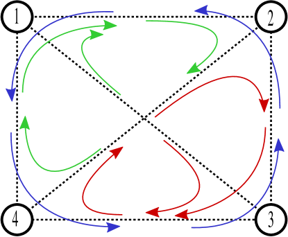
Figure 2: Example of a routing table on a fully connected network with four nodes. There are three distinct cyclic attractors containing the directed links $\big{[}\overrightarrow{(14)},\ \overrightarrow{(43)},\ \overrightarrow{(32)},\ \overrightarrow{(21)}\Big{]}$, $\Big{[}\overrightarrow{(34)},\ \overrightarrow{(42)},\ \overrightarrow{(23)}\Big{]}$ and $\Big{[}\overrightarrow{(12)},\ \overrightarrow{(24)},\ \overrightarrow{(41)}\Big{]}$ respectively. For the nodes 1 and 3 the information centrality is $c=2$, while for nodes 2 and 4 one finds $c=3$.

The rational for these two models in the context of social networks is the following: For the memoryless case a new information is passed on always to the best friend, irrespectively of the information source. In the model with memory the information routing depends on the source. Information received by a relative might be passed on to another relative and work-related news might be passed on predominantly to a work-place buddy. The suppression of backrouting is not important for large $N$ but clearly makes sense; It is never a good idea to echo a joke to the person which told it in the first place.

An example of a routing table on a fully connected graph with four nodes is presented in Fig. 2. In a discrete phase space built upon the directed edges every cycle is an attractor, thus we have cyclic attractors. In this example we have three cyclic attractors (labeled with colors), each of which has a basin of attraction of volume $V=4$, which is the number of directed edges. The states $\overrightarrow{(13)}$ and $\overrightarrow{(31)}$ in the phase space of the dynamics belong to the basin of attractions of the red and the green attractors, respectively, but they do not belong to any cyclic attractor. Also, for nodes 1 and 3 the information centrality $c=2$, while for nodes 2 and 4, $c=3$.

We also note that the vertex routing models (1) play an important role in the context of neural cognitive information processing. In this context a vertex corresponds to an object and the sequence of vertices activated by the routing process to an associative thought process [9, 10]. In addition there is a close relation to random boolean networks [11, 12], with the directed links constituting the boolean variables. In terms of a boolean network the routing model operate in the sparse activity limit, since the routing problem deals with routing of individual packages, a single directed link being operative at any given time.

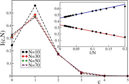
Figure 3: The information centrality $I(c,N)$ for the models with memory, viz the probability that $c$ attractors pass through a given vertex, for $N=10,20,\dots,70$ number of vertices (top-down/down-top for $c=1$/$c=0$). Inset: $I(0,N)$ (red line) and $I(1,N)$ (blue line) as a function of $1/N$, the lines are linear fits.

3 Memoryless model

In this case the routing tensor $T_{ikj}$ is independent of the last index and its dimension is effectively reduced to two. The probability distribution $N_{l}(L,N)$ of finding a cycle of length $L$ in a network with $N$ nodes is given by [see A]

$$N_{l}(L,N)\ =\ {1\over z(N)}\,{N\choose L}{L!\over L}{1\over(N-1)^{L}}~{},$$ (3)

where $z(N)$ is a normalization factor, ${N\choose L}$ the number of $L$ sites out of the $N$ vertices and ${L!/L}$ the number of possibilities to connect $L$ sites into distinct loops. The factor $(N-1)^{-L}$ in (3) is the probability that any ordered set of $L$ sites is connected via the routing table, with $1/(N-1)$ being the probability of two vertices being connected.

For the memoryless model the phase space reduces effectively to the number of vertices $N$, compare Fig. 1, and the cycles are disjoint and non-intersecting, only $c=0,1$ cycles may pass through any vertex in the memoryless model; any given vertex may have only an information centrality $c=0,1$. Defining by $I(c,N)$ the distribution of the information centrality we find [see B]

$$I(1,N)={z(N)\over N}\langle L\rangle=\sum_{L=2}^{N}{(N-1)!\over(N-L)!(N-1)^{L}}$$

for the memoryless model, where we have used (3) and $\langle L\rangle=\sum_{L}LN_{l}(L,N)$. $I(1,N)$ scales like

$$I(1,N)\ \sim\ 1/\sqrt{N},\qquad\quad N\to\infty$$ (4)

in the thermodynamic limit. Only a sub-extensive number of vertices belong to an attractor of the information flow and essentially all vertices are excluded from the long-term flow, $I(0,N)\to 1$ for $N\to\infty$.

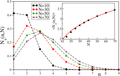
Figure 4: The distribution $N_{a}(n,N)$ of the total number $n$ of cycles per realization, for $N=10,30,50,70$ numbers of vertices. Inset: The average $\langle N_{a}(n,N)\rangle$, as a function of $N$, together with a power-law fit (solid line).

4 Model with memory trace

We have performed extensive numerical simulations of the vertex routing model with a memory trace. We studied ensembles of $N_{real}=10^{6}$ randomly drawn realizations of the routing tensor, considering fully connected networks having $N=10,...,70$ sites, and performing an exhaustive search of all attractors and their respective basins of attractions. We evaluated the normalized distributions

$$I(c,N),\quad N_{a}(n,N),\quad N_{l}(L,N),\quad V_{b}^{max}(v,N)~{},$$ (5)

where $I(c,N)$ is the distribution of the information centrality, with $c$ being the number of attractors passing through a vertex, $N_{a}(n,N)$, the distribution of the number of attractors $n$ per network, $N_{l}(L,N)$ the distribution of the lengths $L$ of attractors and the distribution of the volume of the largest basin of attraction $V_{b}^{max}(v,N)$. For every model realization all basins of attraction were evaluated and the statistics of the maximal volume is given by $V_{b}^{max}(v,N)$, with the volume $v$ being defined relative to the entire phase space $\Omega=N(N-1)$ of directed links.

We find, see Fig. 3, that the information centrality approaches a well defined limiting function $I(c)=\lim_{N\to\infty}I(c,N)$ in the thermodynamic limit. The availability of information is quite democratically distributed, only a fraction $I(0)\approx 0.34$ of vertices are cut-off completely from the long term information flow.

In Fig. 4 the distribution of the number of attractors per network is presented. The average number of attractors per network increases only slowly with the size of the network, as $\langle N_{a}(n,N)\rangle\sim N^{\alpha_{a}}$. Somewhat larger system sizes are necessary for a reliable estimate of the scaling exponent, our best fit (given in the inset of Fig. 4) indicates $\alpha_{a}\approx 0.29$.

We encountered problems of undersampling of the space of all possible model realizations when evaluating the cycle-length distribution $N_{l}(L,N)$, presented in Fig. 5, which is a phenomena well known in the field of random boolean networks [12]. For the case of the vertex routing model the probability of finding very long cycles could not be determined accurately, due to the fat tails of $N_{L}(l,N)$. This problem affects also the results for the mean cycle length $\langle N_{l}(L,N)\rangle$, but not the median $\mu_{a}(N)$ of $N_{l}(L,N)$. We found scaling close to a square-root law for the median (inset of Fig. 5), $\mu_{a}(N)\sim N^{0.51}$.

The number of cyclic attractors steadily increases with $N$, as shown in Fig. 4. The question is then, whether there is typically a single dominating attractor, in terms of the size of the respective basins of attractions, or whether the phase-space volume is more or less equally divided between the attractors being present. This information is provided by $V_{b}^{max}(v,N)$. The probability that the largest attractor volume is in the interval $[v_{1},v_{2}]$ is given by $\sum_{v=v_{1}}^{v_{2}}V_{b}^{max}(v,N)$. Here the volume is relative to the maximal basin of attraction, which is equal to the phase-space volume $\Omega=N(N-1)$ and $v=1$ occurs when only a single attractor is present.

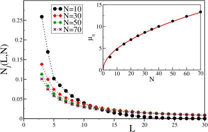
Figure 5: The cycle-length distribution $N_{l}(L,N)$ as a function of cycle length $L$, for $N=10,20,\dots,70$ number of vertices. Inset: The median $\mu_{a}(N)$ of $N_{l}(L,N)$, as a function of $N$.

The rescaled $\Omega V_{b}^{max}(v,N)$ converges rapidly with $N$ to a limiting function, see Fig. 6. There is a divergence for $v\to 1$, due to the fact that the probability of finding an ensemble realization with a single attractor, $N_{a}(1,N)$, scales like $1/N$ and consequently $\Omega V_{b}^{max}(v=1,N)=\Omega N_{a}(n=1,N)\sim N$. A kink at $v=1/2$ occurs for $V_{b}^{max}(v,N)$. For $v>1/2$ ensemble realizations containing two or more cycles contribute to $V_{b}^{max}(v,N)$, for $v<1/2$ realizations with three or more attractors contribute.

The divergence of $\Omega V_{b}^{max}(v,N)$ for $v\to 1$ seems to indicate that cycles with large volumes of attraction would have a dominating role, controlling most of the long-term information flow. In order to understand the origin of this divergence we have compared the integrated distribution $\int_{0}^{v}dv^{\prime}V_{b}^{max}(v^{\prime},N)$ (inset of Fig. 6) with an unbiased distribution of basins of attraction, taking the case of two attractors (dashed line in the inset of Fig. 6). In this case, when only two attractors are present, one of the volumes of attraction is always equal or larger than $\Omega/2$, and

$$\int_{0}^{v}dv^{\prime}V_{b}^{max}(v^{\prime},N)\ =\ \left\{\begin{array}[]{rcl}0&&v<1/2\\ 2v-1&&v>1/2\end{array}\right.~{}.$$ (6)

The integrated distribution of model with a memory trace follows somewhat the simplified model (6) of a random distribution of two basins of attraction, albeit with a substantial suppression close to unity, indicating that the divergence of $\Omega V_{b}^{max}(v,N)$ for $v\to 1$ is a directly related to the statistical properties of the distribution of basins of attraction, independent of the details of the dynamics.

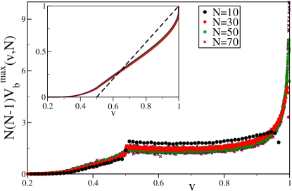
Figure 6: The rescaled distribution $N(N-1)V_{b}^{max}(v,N)$ of the volumes of the basin of attractions, for $N=10,30,50,70$. The volume $v$ is normalized with respective to the total phase space $\Omega=N(N-1)$ of directed links. Inset: The integrated distribution $\int_{0}^{v}dv^{\prime}V_{b}^{max}(v^{\prime},N)$, for $N=30,50,70$ (the curves fall on top of each other). For comparison the result (6) for the case of two attractors with randomly distributed basins of attractions is given (dashed line).

5 Discussion

We have presented and analyzed a novel class of models suitable for describing the flow of information in complex networks. In these models the flow of information is realized by information packages travelling along the edges of a communication network, whereas it is assumed, in the intensively studied information diffusion models, that information is an attribute attached to the vertices and not to the edges. The dynamics is determined in our class of models by routing tables, specifying respectively for every vertex the routing of incoming information packages.

The two vertex routing models discussed in the present study constitute idealized reference models, not suitable for a direct modeling of field data. The key point of the present study is to analyze the non-trivial effects of a memory trace on the long-term information flow and not the dependence on the network topology, which is left for further studies. Information is conserved in the present models. This would be clearly not the case for real-world social networks but it holds for the network of internet routers, which have the task of routing packages of information without increasing or decreasing their number.

Traditionally, the flow of information in social networks, like the random spreading of rumors, has been modeled by diffusion processes [13]. Searching for more realistic models the special topology of social networks has been discussed intensively [14], as well as corrections to the diffusion process itself [15]. The vertex routing and the diffusion models of information flow constitute two extremes. In the first model the direction of the information flow is 100% deterministic, in the second model 100% random. The information-flow occurring in real-world social nets is expected to be partially a random and partially a directed process. It will therefore be of interest for future studies to interpolate between these two reference models. We propose that field studies characterizing social networks should be supplemented by data describing the dynamics of the information flow, in addition to the standard structural and topological characterization, as the accumulation of information in the attractors of the information flow may have a substantial social impact.

The dependence of the routing dynamics on the network topology is additionally an important issue for future studies. Cycles in the routing process can only then appear, when the underlying network topology allows for loops. Here we have been considering fully connected networks and loops of all length are present. For many classes of real-world networks there is a characteristic loop-length, which generally scales sub-extensively with the network-size [16]. Interesting interferences phenomena between this scaling and the sub-extensive scaling of the typical attractor-length (inset of Fig. 5) may then be expected.

Appendix A The cycle length distribution for the memoryless model

Let $q_{t}$ be the probability that a path remains unclosed after t steps. If a path is still open at time $t$, we have already visited $t+1$ different nodes. There are $t$ ways to close the path in the next time step. The relative probability is then $\rho_{t}=t/(N-1)$. The probability of still having an open path after $t$ steps is

$$q_{t+1}=q_{t}(1-\rho_{t})=\prod_{i=0}^{t}\Big{(}\frac{N-i-1}{N-1}\Big{)},\qquad q_{0}=1$$

$$\Rightarrow\qquad q_{t}=\frac{(N-1)!}{(N-1)^{t}(N-1-t)!}~{}.$$

The average number of cycles of length $L$ is

$$\langle N_{l}(L)\rangle=\frac{q_{t=L-1}}{N-1}\frac{N}{L}=\frac{N!}{L(N-1)^{L}(N-L)!}~{},$$

where we used the following considerations [4]:

1. The probability that the node, visited at time $t+1$, is identical to the starting node is $1/(N-1)$.

2. There are $N$ possible starting points.

3. Factor $1/L$ corrects for the overcounting of cycles when considering the L possible starting sites of the L-cycle.

After normalization we obtain Eq. (3) , the probability distribution of cycle lengths

$$N_{l}(L,N)=\frac{1}{z(N)}\frac{N!}{L(N-1)^{L}(N-L)!}~{},$$

where $z(N)$ is normalization factor

$$z(N)=\sum_{L=2}^{N}\frac{N!}{L(N-1)^{L}(N-L)!}=\frac{N!}{(N-1)^{N}}\sum_{k=0}^{N-2}\frac{(N-1)^{k}}{(N-k)k!}~{}.$$

Appendix B Connection between the average information centrality and the average cycle length

We consider an ensemble of $R$ random realizations of a routing tensor on a fully connected network with $N$ nodes. Let $n_{\alpha}$ be the total number of vertices which belong to at least one cyclic attractor, where $\alpha=1\ldots R~{}$.

The length of an cyclic attractor is equivalent to the number of vertices that belong to the attractor. In the case of only one existing attractor $n_{\alpha}=L-\sum_{r=1}^{r_{max}}(r-1)Q_{\alpha}(r,N)$, where L is the length of the attractor and $Q_{\alpha}(r,N)$ is the number of nodes which are repeated $r$ times during one cycle of the cyclic attractor. If we denote the number of cycles of length $L$ with $N_{\alpha}(L,N)$, we can write, for the case of more than one co-existing cyclic attractors, the following relation

$$n_{\alpha}=\sum_{L}LN_{\alpha}(L,N)-\sum_{r=1}^{r_{max}}(r-1)Q_{\alpha}(r,N)-\sum_{c=1}^{c_{max}}(c-1)P_{\alpha}(c,N)~{},$$ (7)

where $P_{\alpha}(c,N)$ is number of nodes with information centrality $c$. For example let us consider the case when we have two attractors [$\overrightarrow{(12)}$, $\overrightarrow{(23)}$, $\overrightarrow{(31)}$ ] and [$\overrightarrow{(14)}$, $\overrightarrow{(45)}$, $\overrightarrow{(51)}$, $\overrightarrow{(16)}$, $\overrightarrow{(67)}$, $\overrightarrow{(71)}$]. It is easy to count that there are 7 distinct vertices contained in this two attractors. We see that only node 1 has information centrality c=2, thus $P_{\alpha}(c=1)=6$ and $P_{\alpha}(c=2)=1$. Also, node 1 is the only one two repeat two times during one cycle of second attractor, thus $Q_{\alpha}(r=1)=6$ and $Q_{\alpha}(r=2)=1~{}$. If we put this values into (7) we obtain $n_{\alpha}=7$.

On the other hand, if we denote the distribution presented in Fig. 3 as $I(c,N)$, where $c$ is the information centrality, then, in the case of one given realization of the routing tensor, we can write

$$P_{\alpha}(c,N)=N\cdot I_{\alpha}(c,N)~{}.$$ (8)

Also, total number of vertices, which are members of cyclic attractors, is then

$$n_{\alpha}=N\sum_{c=1}^{c_{max}}I_{\alpha}(c,N)~{}.$$ (9)

Combining (7) and (8) with (9) we obtain

$$N\sum_{c=1}^{c_{max}}I_{\alpha}(c,N)= \sum_{L}LN_{\alpha}(L,N)-N\sum_{c=1}^{c_{max}}(c-1)I_{\alpha}(c,N)-$$

$$-\sum_{r=1}^{r_{max}}(r-1)Q_{\alpha}(r,N)~{},$$

After averaging over entire ensemble of $R$ realizations of routing tensor and dividing both sides of (B) with $N$, we obtain

$$\sum_{c=1}^{c_{max}}cI(c,N)=\frac{z(N)}{N}\sum_{L}LN_{l}(L,N)-\frac{1}{N}\sum_{r=1}^{r_{max}}(r-1)Q(r,N)~{},$$ (11)

where we have used following relations

$$\frac{1}{R}\sum_{\alpha=1}^{R}N_{\alpha}(L,N)=z(N)\cdot N_{l}(L,N)~{},$$

$$\frac{1}{R}\sum_{\alpha=1}^{R}I_{\alpha}(c,N)=I(c,N)~{},$$

$$\frac{1}{R}\sum_{\alpha=1}^{R}Q_{\alpha}(c,N)=Q(c,N)~{}.$$

In the case of the memoryless model, $I(c,N)$ have non zero values only for $c=0,1$, and it is not possible that one node is repeated more than once in one cycle of cyclic attractor, thus $\frac{1}{N}\sum_{r}(r-1)Q(r,N)=0$. Therefore, from (11) we obtain

$$I(1,N)=\frac{z(N)}{N}\langle L\rangle~{},$$ (12)

where $\langle L\rangle=\sum_{L}LN_{l}(L,N)~{}$, which is the central result of this appendix.

References

References

- [1] R. Albert and A. Barabàsi, Statistical mechanics of complex networks, Reviews of Modern Physics 74, 47 (2002).
- [2] S.N. Dorogovtsev and J.F.F. Mendes, Evolution of networks Advances in Physics 51, 1079 (2002).
- [3] S. Boccaletti, V. Latora, Y. Moreno, M. Chavez and D.U.Hwang, Complex networks: Structure and dynamics, Physics Reports 424, 175 (2006).
- [4] C. Gros, Complex and Adaptive Dynamical Systems, A Primer, Springer (2008).
- [5] M.S. Granovetter, The Strength of Weak Ties, American Journal of Sociology 78, 1360 (1973).
- [6] S. Wasserman and K. Faust, Social Network Analysis: Methods and Applications, Cambridge University Press (1994).
- [7] P. Erdös and A. Rényi, On random graphs Publicationes Mathematicae 6, 290 (1959).
- [8] S.A. Kauffman, Metabolic Stability and Epigenesis in Randomly Constructed Nets, Journal of Theoretical Biology 22, 437 (1969).
- [9] C. Gros, Neural networks with transient state dynamics, New Journal of Physics 9, 109 (2007).
- [10] C. Gros, Cognitive computation with autonomously active neural networks: an emerging field, Cognitive Computation 1, 77 (2009).
- [11] M. Aldana-Gonzalez, S. Coppersmith and L.P. Kadanoff, Boolean Dynamics with Random Couplings, in E. Kaplan, J.E. Marsden, K.R. Sreenivasan (eds.), Perspectives and Problems in Nonlinear Science, Springer (2003).
- [12] B. Drossel, Random Boolean Networks, in H.G. Schuster (ed), Reviews of Nonlinear Dynamics and Complexity 1 (2008).
- [13] J.P. Cointet, and C. Roth, How Realistic Should Knowledge Diffusion Models Be?, Journal of Artificial Societies and Social Simulation 10, 3 (2007).
- [14] M.E.J. Newman, The Structure and Function of Complex Networks, SIAM Review 45, 167 (2003).
- [15] F. Wu, B.A. Huberman, L.A. Adamic, and J.R. Tyler, Information flow in social groups, Physica A 337, 1 (2004).
- [16] H.D. Rozenfeld, J.E. Kirk, E.M. Bollt, and D. Ben-Avraham, Statistics of cycles: How loopy is your network?, J.Phys. A: Math. Gen. 38, 4589-4595 (2005)