The Role of Anisotropy in the Void Models without Dark Energy

Abstract

Void models provide a possible explanation of the “accelerated expansion” of the Universe without dark energy. To make the conventional void models more realistic, we allow the void, an underdense region around us, to be anisotropic and consider an average of the distance-redshift relations over the solid angle subtended at the observer. We first show that after taking the average of a form of the optical scalar equation (distance equation), the effective distance equation we obtain coincides with the one for the Lemaître-Tolman-Bondi universe with a Dyer-Roeder-like extension. We then numerically solve the equation to compare with observational data of Type Ia supernovae. We find that anisotropy allows smaller size of void and larger $\Omega_{m}$.

1 Introduction

In recent years, reliable distance-redshift relations up to $z\sim 1$ have been revealed by observations of Type Ia supernovae [1, 2]. Comparisons of the data obtained from these observations with the predictions from Friedmann-Lemaître (FL) homogeneous and isotropic universe models suggest that the Universe is in a phase of accelerated expansion, and there must exist unidentified dark energy that causes the acceleration. The nature of dark energy has been investigated by many researchers [3].

On the other hand, the possibilities have been discussed that the distance-redshift relations provided by the observations of Type Ia supernovae may be reproduced by taking account of the inhomogeneities in the matter distribution and geometry without dark energy. One of such models is the so-called void model, in which existence of a large scale underdense region (void) is assumed. Actually, an inhomogeneous distribution of matter of scale $200\sim 300/h$ Mpc (the Hubble constant is $100h$ km/s/Mpc) was suggested by several authors [4] in galactic surveys, and a void on scales of about $250/h$ Mpc was found by Blanton et al. [5] in the SDSS commissioning data. These results suggest that we might live in a local void with a radius of $200\sim 300/h$Mpc. Motivated by these observations, Tomita [6, 7, 8] sought to reproduce the distance-redshift relations using a model in which a homogeneous spherical region around us is less dense than the background.

More recently, Alnes et al. [9] (also, [10, 11]) showed that there exists a model that provides a good fit to the Type Ia supernova observations (as well as other kinds), assuming that the outside of a spherical region is homogeneous and isotropic but the inside of it is described by the Lemaitre-Tolman-Bondi (LTB) spherically symmetric dust solution [12, 13, 14]. Yoo et al. [15] showed that if the arbitrary functions in the LTB solution are determined so that the distance-redshift relation in the LTB spacetime coincides with that of the $\Lambda$CDM model, the resulting model has a void structure on scales of a few Gpc.

The essential mechanism for these void models to be able to reproduce the distance-redshift relations provided by the observations is that the local Hubble expansion rate monotonically decreases as the distance increases so that the incoming light rays experience effective increase in the expansion rate.

In reality, however, the matter distribution in the Universe is not isotropic, and the distance-redshift relation inferred by the observational data should be considered as an average over all the directions of sight. This point seems to have been largely ignored in the literature. To take into account the effect caused by these anisotropies, we in this paper start with the optical scalar equation in general inhomogeneous and anisotropic spacetimes, and then take an average of a form of this equation (distance equation) over the spheres on the past light cone. We find that after some estimates, the resulting equation coincides with the one in the LTB universe with the matter density $\rho_{\text{LTB}}$ formally replaced by $\alpha(z)\rho_{\text{LTB}}$, where $\alpha(z)$ is a certain function of $z$. In other words, the equation coincides with the one obtained as a Dyer-Roeder-like [16, 17] extension of the distance equation in the LTB universe. With this effective equation, we numerically investigate light properties of void models including effects of anisotropy.

Mattsson [18] has recently discussed a similar generalization of the Dyer-Roeder equation, arguing principally that the original Dyer-Roeder extension did not take into account spatial inhomogeneities in expansion rate. To incorporate these inhomogeneities, he replaced the Hubble expansion rate $H_{\text{FL}}$ in the Dyer-Roeder equation with $\beta_{\text{M}}(z)H_{\text{FL}}$, with $\beta_{\text{M}}(z)$ being an arbitrary function of $z$. We do not have to artificially introduce a phenomenological function like $\beta_{\text{M}}(z)$, since we start with a general inhomogeneous and anisotropic setting, which naturally leads to an equation with the effect of inhomogeneities in both matter density and expansion rate. Moreover, the inhomogeneity and anisotropy we consider is supposed to be made by smooth distribution of dark matter, rather than the spiky clumpiness by galaxies as assumed in Mattsson [18] and in Dyer and Roeder [16, 17].

This paper is organized as follows. In section 2, we derive our effective distance equation by means of averaging. In section 3, we consider a specific void model and numerically solve the effective distance equation to search the parameter space for the best values that are most likely to explain observational data. Section 4 is devoted to conclusion and some remarks. Appendix A provides a review for the original Dyer-Roeder extension. Throughout this paper, we use $c=1$ as the speed of light.

2 The effective distance equation for inhomogeneious and anisotropic spacetimes

In the first subsection below, we transform the optical scalar equation to derive an equation for the angular-diameter distance $D_{A}$ in an inhomogeneous and anisotropic dust universe. We then specialize the equation to the LTB spherically symmetric dust universe case for later use. In the second subsection, we take a spherical average of the general distance equation to make the equation suitable for comparisons with observational data.

2.1 Distance equation and its specialization in the LTB spacetime

We start with the optical scalar equation [19], which determines the variations of the cross sectional area of a null geodesic congruence. Let us assume that the null geodesics in the congruence arrive at the observer through paths that are sufficiently far from strong inhomogeneities such as galaxies. This allows us to ignore the gravitational lensing effect, and in turn, the shear and rotation of the congruence. The optical scalar equation in this case becomes

$$\frac{2}{\sqrt{A}}\frac{d^{2}\sqrt{A}}{d\lambda^{2}}+R_{\mu\nu}k^{\mu}k^{\nu}=0,$$ (1)

where $A$ is the cross sectional area of the congruence, $k^{\mu}$ the null geodesic generator, $\lambda$ the affine parameter, and $R_{\mu\nu}$ the Ricci tensor. On the other hand, Einstein’s equation

$$R_{\mu\nu}-\frac{1}{2}Rg_{\mu\nu}=8\pi GT_{\mu\nu},$$ (2)

where $T_{\mu\nu}$ is the energy momentum tensor, implies

$$R_{\mu\nu}k^{\mu}k^{\nu}=8\pi GT_{\mu\nu}k^{\mu}k^{\nu},$$ (3)

since $k^{\mu}$ is null. With the relation $D_{A}\propto\sqrt{A}$ for the angular diameter distance $D_{A}$, we obtain

$$\frac{2}{D_{A}}\frac{d^{2}D_{A}}{d\lambda^{2}}+8\pi GT_{\mu\nu}k^{\mu}k^{\nu}=0$$ (4)

from Eqs.(1) and (3). The only energy content we consider is dust, so that $T_{\mu\nu}=\rho u^{\mu}u^{\nu}$, where $\rho$ is the energy density for dust, $u^{\mu}$ the 4-velocity of dust. The frequency of the light observed by a comoving observer at a given $\lambda$ with 4-velocity $u^{\mu}$ is given by $\omega(\lambda)=-u_{\mu}k^{\mu}$ (e.g., [20]). Therefore the second term in the left hand side of Eq.(4) yields

$$T_{\mu\nu}k^{\mu}k^{\nu} =\omega(\lambda)^{2}\rho$$

$$=\omega(0)^{2}(1+z)^{2}\rho,$$ (5)

where we have used the definition of redshift $z$, $z\equiv\frac{\omega(\lambda)}{\omega(0)}-1$. Thus, Eq.(4) can be written as

$$\mathcal{L}^{2}D_{A}+4\pi G\rho D_{A}=0,$$ (6)

where $\mathcal{L}^{2}$ is the second order linear derivative operator defined by

$$\mathcal{L}^{2}\equiv\frac{1}{\omega^{2}(0)(1+z)^{2}}\frac{d^{2}}{d\lambda^{2}}.$$ (7)

We stress that this equation is valid for any dust universe, as long as the gravitational lensing effect along the geodesics we consider can be ignored. Note also that solving this equation requires another equation (geodesic equation) to relate $\lambda$ with $z$, for given $\rho$.

Next, we specialize the last equation to the LTB spherically symmetric spacetime case with the observer at the symmetry center. The essential part of our task is to convert $d/d\lambda$ to $d/dz$ for the case.

The LTB metric is given by

$$ds^{2} =-dt^{2}+\frac{(R^{\prime}(t,r))^{2}}{1+2E(r)}dr^{2}+R(t,r)^{2}d\Omega^{2},$$ (8)

where the ‘energy function’ $E(r)$ is an arbitrary function concerning curvature. The circumferential radius $R(t,r)$ is the solution for the generalized Friedmann equation

$$\frac{1}{2}\dot{R}^{2}(t,r)-\frac{M(r)}{R(t,r)}=E(r),$$ (9)

where the ‘mass function’ $M(r)$ is another arbitrary function, and $\dot{}$ and ^′ denote the derivatives with respect to $t$ and $r$, respectively.

Using the analytic function $\mathcal{S}(x)$ introduced in Ref.[21], the solution $R$ can be represented simply as

$$R(t,r)=(6M(r))^{1/3}(t-t_{B}(r))^{2/3}\mathcal{S}\left(-2E(r)\left(\frac{t-t_{B}(r)}{6M(r)}\right)^{2/3}\right),$$ (10)

where the ‘Big-Bang function’ $t_{B}(r)$ is a third arbitrary function. The function $\mathcal{S}(x)$ is the unique solution of the first order ordinary differential equation

$$\frac{4}{3}(\mathcal{S}(x)+x\frac{d\mathcal{S}(x)}{dx})^{2}+3x-\frac{1}{\mathcal{S}(x)}=0$$ (11)

that intersects the $x=0$ axis transversely [21]. This function is non-negative, monotonically decreasing, and defined for $x\leq(\pi/3)^{2/3}$.

As for the dust matter, the 4-velocity is given by $u^{\mu}=(1,0,0,0)$, and the energy density by

$$4\pi\rho_{\text{LTB}}(t,r)=\frac{M^{\prime}(r)}{R^{\prime}(t,r)R^{2}(t,r)}.$$ (12)

Now, suppose that the light we observe progresses along a path $x^{\mu}(\lambda)$ for decreasing $\lambda$ with $\lambda=0$ corresponding to the observer, so that $k^{\mu}=-dx^{\mu}/d\lambda$. Then, we obtain

$$\frac{d}{d\lambda} =\frac{dz}{d\lambda}\frac{d}{dz}=\frac{1}{\omega(0)}\frac{d\omega(\lambda)}{d\lambda}\frac{d}{dz}$$

$$=\frac{-1}{\omega(0)}\left(\frac{d^{2}t}{d\lambda^{2}}\right)\frac{d}{dz},$$ (13)

since $\omega(\lambda)=k^{0}(\lambda)=-dt/d\lambda$. On the other hand, the radial geodesic equation for $t(\lambda)$ and the null condition, respectively, give us

$$\frac{d^{2}t}{d\lambda^{2}} =\frac{-R^{\prime}\dot{R^{\prime}}}{1+2E}\left(\frac{dr}{d\lambda}\right)^{2}, -\left(\frac{dt}{d\lambda}\right)^{2}+\frac{R^{\prime 2}}{1+2E}\left(\frac{dr}{d\lambda}\right)^{2} =0.$$ (14)

Using these equations, we immediately have

$$\frac{d}{d\lambda} =\frac{1}{\omega(0)}\frac{\dot{R^{\prime}}}{R^{\prime}}\left(\frac{dt}{d\lambda}\right)^{2}\frac{d}{dz}$$

$$=\omega(0)\frac{\dot{R^{\prime}}}{R^{\prime}}(1+z)^{2}\frac{d}{dz}$$

$$=\omega(0)H_{\text{LTB}}(z)(1+z)^{2}\frac{d}{dz},$$ (15)

where we have defined the effective Hubble function $H_{\text{LTB}}$,

$$H_{\text{LTB}}=\frac{\dot{R^{\prime}}}{R^{\prime}}.$$ (16)

Consequently, Eq.(6) yields

$$\mathcal{L}^{2}_{\text{LTB}}D^{(\text{LTB})}_{A}(z)+4\pi G\rho_{\text{LTB}}(z)D^{(\text{LTB})}_{A}(z)=0,$$ (17)

where

$$\mathcal{L}^{2}_{\text{LTB}}\equiv H_{\text{LTB}}(z)\frac{d}{dz}\left[H_{\text{LTB}}(z)(1+z)^{2}\frac{d}{dz}\right],$$ (18)

and $D^{(\text{LTB})}_{A}$ represents the angular-diameter distance in the LTB universe. Note that this equation is the same as the one for the FL universe (See Eq.(62) in appendix A) with the Hubble function replaced by Eq.(16). (This is the reason we call $H_{\text{LTB}}$ the effective Hubble function.) Note also that the effective Hubble function $H_{\text{LTB}}(z)$ coincides with the so-called longitudinal Hubble function $H_{\parallel}\equiv{\dot{R^{\prime}}}/{R^{\prime}}$; in contrast, the perpendicular Hubble function $H_{\perp}\equiv\dot{R}/R$ plays no role in determining the distance.

2.2 Averaging of anisotropies

In this subsection, we take a spherical average of the distance equation (6) and compare it with the one for the isotropic spacetime Eq.(17).

For our purpose, the most convenient is to take a particular coordinate system that is based on a foliation of spacetime by past light cones of a timelike curve. We employ a spherical null coordinate system $(\tau,z,\theta,\phi)$ such that $\tau=\text{constant}$ on each light cone, that $z=0$ corresponds to the vertex of each light cone, that the timelike curve the vertices $z=0$ comprise coincides with the orbit of matter flow there, and that the angular coordinates $(\theta,\phi)$ are constant along each null geodesic that reaches the vertex $z=0$. (This choice of angular coordinates is possible at least in the domain where the null geodesics do not intersect each other.) The radial null coordinate $z$ is chosen to give the redshift along each null geodesic labeled by $(\tau,\theta,\phi)$. Our observation is supposed to be done at the coordinate center $z=0$ at a certain instant $\tau=\tau_{0}$.

Let $D_{A}(z\,;\theta,\phi)$ be the angular-diameter distance to an object observed in the direction $(\theta,\phi)$ with redshift $z$. This is a function of $z$, $\theta$, and $\phi$, but we will often regard this as a function of $z$ with $\theta$ and $\phi$ being parameters, since we mostly consider its variations along the null geodesic, in which situation $\theta$ and $\phi$ are constant. We will therefore use $d/dz$ instead of $\partial/\partial z$ when it acts on $D_{A}(z\,;\theta,\phi)$. The same rule will be applied to other functions as well.

Let us define the spherical average of a function $f(z\,;\theta,\phi)$ by

$$\bar{f}(z)\equiv\langle f(z;\theta,\phi)\rangle\equiv\frac{1}{4\pi}\int f(z;\theta,\phi)d\Omega,$$ (19)

where $d\Omega\equiv\sin\theta d\theta d\phi$. Then, the spherical average of Eq.(6) can be written as

$$\langle\mathcal{L}^{2}D_{A}(z;\theta,\phi)\rangle+4\pi G\langle\rho(z;\theta,\phi)D_{A}(z;\theta,\phi)\rangle=0.$$ (20)

Here, the derivative operator $\mathcal{L}^{2}$ becomes under our coordinates

$$\begin{split}\mathcal{L}^{2}&=\frac{1}{\omega^{2}(0)(1+z)^{2}}\left(\frac{dz}{d\lambda}\frac{d}{dz}\right)^{2}\\ &=H(z\,;\theta,\phi)\frac{d}{dz}\left[H(z\,;\theta,\phi)(1+z)^{2}\frac{d}{dz}\right],\end{split}$$ (21)

where the general Hubble function $H(z\,;\theta,\phi)$ is defined by

$$H(z\,;\theta,\phi)\equiv\frac{1}{\omega(0)(1+z)^{2}}\frac{dz}{d\lambda}.$$ (22)

Note that in the averaged equation (20), each term in the left hand side depends only on $z$, as in the LTB equation (17). We wish to estimate how much different the averaged distance function $\bar{D}_{A}(z)=\langle D_{A}(z\,;\theta,\phi)\rangle$ is from an LTB distance function $D^{\text{(LTB)}}_{A}(z)$. To this, we match an LTB solution with the given inhomogeneous and anisotropic universe according to the following correspondence:

$$\bar{\rho}(z)=\rho_{\text{LTB}}(z),\quad\bar{H}(z)=H_{\text{LTB}}(z).$$ (23)

Since the LTB solution possesses two arbitrary physical functions (one of the three arbitrary functions corresponds to gauge), it is natural to expect that these two conditions are satisfied for a suitable choice of these functions. (Strictly speaking, asserting this leads to a variation of the inverse problem for the LTB solution, which we consider out of our scope. For a discussion of the standard version of the inverse problem, see, e.g., [22].)

Keeping this correspondence in mind, we formally rewrite equation (20) in the form

$$\langle\mathcal{L}^{2}D_{A}\rangle(z)+4\pi G\alpha(z)\rho_{\text{LTB}}(z)\bar{D}_{A}(z)=0,$$ (24)

where

$$\alpha(z) \equiv\frac{\langle\rho(z;\theta,\phi)D_{A}(z;\theta,\phi)\rangle}{\rho_{\text{LTB}}(z)\bar{D}_{A}(z)}.$$ (25)

To evaluate the average $\langle\mathcal{L}^{2}D_{A}\rangle$ and the ratio function $\alpha(z)$, let us decompose physical functions as

$$\rho(z;\theta,\phi) =\rho_{LTB}(z)[1+\delta_{\rho}(z;\theta,\phi)],$$ (26)

$$H(z;\theta,\phi) =H_{\text{LTB}}(z)[1+\delta_{H}(z;\theta,\phi)],$$ (27)

$$D_{A}(z;\theta,\phi) =\bar{D}_{A}(z)[1+\delta_{D}(z;\theta,\phi)],$$ (28)

where $\langle\delta_{*}\rangle=0\,(*=\rho,H,\text{or }D)$. To calculate the quantity $\mathcal{L}^{2}D_{A}$, it is most convenient to use the following identity that is confirmed by a straightforward computation;

$$\mathcal{L}^{2}=(1+\delta_{H})^{2}\mathcal{L}_{\text{LTB}}^{2}+H_{\text{LTB}}^{2}(1+z)^{2}[\delta_{H}^{\prime}+\frac{1}{2}(\delta_{H}^{2})^{\prime}]\frac{d}{dz}.$$ (29)

Here, a prime stands for $d/dz$. Using this formula we can calculate

$$\begin{split}\mathcal{L}^{2}D_{A}=&\mathcal{L}^{2}\bar{D}_{A}(1+\delta_{D})\\ =&(\mathcal{L}^{2}\bar{D}_{A})(1+\delta_{D})+\bar{D}_{A}\mathcal{L}^{2}(1+\delta_{D})+2H_{\text{LTB}}^{2}(1+\delta_{H})^{2}(1+z)^{2}\bar{D}_{A}^{\prime}\delta_{D}^{\prime}\\ =&(1+\delta_{H})^{2}[(1+\delta_{D})\mathcal{L}_{\text{LTB}}^{2}\bar{D}_{A}+\bar{D}_{A}\mathcal{L}_{\text{LTB}}^{2}\delta_{D}]\\ &+H_{\text{LTB}}^{2}(1+z)^{2}(\delta_{H}^{\prime}+\frac{1}{2}(\delta_{H}^{2})^{\prime})[(1+\delta_{D})\bar{D}_{A}^{\prime}+\bar{D}_{A}\delta_{D}^{\prime}]\\ &+2H_{\text{LTB}}^{2}(1+z)^{2}(1+\delta_{H})^{2}\bar{D}_{A}^{\prime}\delta_{D}^{\prime}.\end{split}$$ (30)

(To obtain the second line, Leibniz’s rule was applied.) Taking average of this equation leads to an expression for $\langle\mathcal{L}^{2}D_{A}\rangle$, which we, for convenience, write in three parts depending on order in $\delta_{*}$;

$$\langle\mathcal{L}^{2}D_{A}\rangle=\mathcal{L}_{\text{LTB}}^{2}\bar{D}_{A}+O(2)+O(3),$$ (31)

where $O(2)$ and $O(3)$ are, respectively, the second and third order term. Brief calculations show that

$$\begin{split}O(2)=&\,(\langle\delta_{H}^{2}\rangle+2\langle\delta_{H}\delta_{D}\rangle)\mathcal{L}_{\text{LTB}}^{2}\bar{D}_{A}\\ &+H_{\text{LTB}}^{2}(1+z)^{2}(\langle\delta_{H}\delta_{H}^{\prime}\rangle+4\langle\delta_{H}\delta_{D}^{\prime}\rangle+\langle\delta_{H}^{\prime}\delta_{D}\rangle)\bar{D}_{A}^{\prime}\\ &+\bigg{(}2\langle\delta_{H}\mathcal{L}_{\text{LTB}}^{2}\delta_{D}\rangle)+H_{\text{LTB}}^{2}(1+z)^{2}\langle\delta_{H}^{\prime}\delta_{D}^{\prime}\rangle\bigg{)}\bar{D}_{A},\end{split}$$ (32)

and

$$\begin{split}O(3)=&\,\langle\delta_{H}^{2}\delta_{D}\rangle\mathcal{L}_{\text{LTB}}^{2}\bar{D}_{A}\\ &+H_{\text{LTB}}^{2}(1+z)^{2}(\langle\delta_{H}\delta_{H}^{\prime}\delta_{D}\rangle+2\langle\delta_{H}^{2}\delta_{D}^{\prime}\rangle)\bar{D}_{A}^{\prime}\\ &+\bigg{(}\langle\delta_{H}^{2}\mathcal{L}_{\text{LTB}}^{2}\delta_{D}\rangle+H_{\text{LTB}}^{2}(1+z)^{2}\langle\delta_{H}\delta_{H}^{\prime}\delta_{D}^{\prime}\rangle\bigg{)}\bar{D}_{A}.\end{split}$$ (33)

Since the perturbation of distance is mainly caused by a perturbation of the expansion rate, we may have $\delta_{D}\sim\delta_{H}$ as a rough estimate. Simplifying the second order term according to this approximation and omitting the third order term, we have

$$\begin{split}\langle\mathcal{L}^{2}D_{A}\rangle\simeq&\,(1+3\langle\delta_{H}^{2}\rangle)\mathcal{L}_{\text{LTB}}^{2}\bar{D}_{A}+3H_{\text{LTB}}^{2}(1+z)^{2}\langle\delta_{H}^{2}\rangle^{\prime}\bar{D}_{A}^{\prime}\\ &+\bigg{(}2\langle\delta_{H}\mathcal{L}_{\text{LTB}}^{2}\delta_{H}\rangle+H_{\text{LTB}}^{2}(1+z)^{2}\langle\delta_{H}^{\prime 2}\rangle\bigg{)}\bar{D}_{A}.\end{split}$$ (34)

On the other hand, the function $\alpha(z)$ can be simply calculated as

$$\alpha(z) =\frac{1}{\rho_{LTB}(z)\bar{D}_{A}(z)}\big{\langle}\rho_{LTB}(z)[1+\delta_{\rho}(z;\theta,\phi)]\,\bar{D}_{A}(z)[1+\delta_{D}(z;\theta,\phi)]\big{\rangle}$$

$$=1+\langle\delta_{\rho}\delta_{D}\rangle.$$ (35)

The fact that the emptier the region the light we observe travels, the longer the distance from the light source implies that $\delta_{\rho}$ and $\delta_{D}$ have an opposite sign each other. Therefore we have

$$\alpha(z)\leq 1$$ (36)

with equality being satisfied only in the LTB isotropic universe.

Furthermore, according to the CMB observation, the perturbation of the expansion rate is about $|\delta_{H}|\equiv\sqrt{\langle\delta_{H}^{2}\rangle}\sim 0.1$ [23] on scales of $z\sim 0.1$, which implies that the second order terms in $\langle\mathcal{L}^{2}D_{A}\rangle$ are much smaller than the second order term in $4\pi G\alpha(z)\rho_{\text{LTB}}\bar{D}_{A}$ if $|\delta_{\rho}|\sim 1$. We therefore neglect the second order terms in $\langle\mathcal{L}^{2}D_{A}\rangle$ and simply have

$$\langle\mathcal{L}^{2}D_{A}\rangle\simeq\mathcal{L}_{\text{LTB}}^{2}\bar{D}_{A}.$$ (37)

We also note that if $|\delta_{D}|\sim|\delta_{H}|\sim 0.1$ and $|\delta_{\rho}|\sim 1$, then Schwarz’s inequality implies $|\langle\delta_{\rho}\delta_{D}\rangle|\leq|\delta_{\rho}||\delta_{D}|\sim 0.1$, or

$$\alpha(z)\gtrsim 0.9.$$ (38)

To summarize, the distance equation (24) takes the form

$$\mathcal{L}^{2}_{\text{LTB}}\bar{D}_{A}(z)+4\pi G\alpha(z)\rho_{\text{LTB}}(z)\bar{D}_{A}(z)=0,$$ (39)

where $\alpha(z)$ is a function in the range

$$0.9\lesssim\alpha(z)\leq 1.$$ (40)

Equation (39) is the effective distance equation the averaged distance function $\bar{D}_{A}(z)$ should satisfy. We will use this equation to determine an LTB solution and the function $\alpha(z)$, comparing its solution $\bar{D}_{A}(z)$ with a set of observational data.

Finally, we discuss another possibility where $\alpha(z)$ can be smaller than $0.9$. Note that if the directions for which the Type Ia supernovae are observed were biased, we would have to restrict the integration region from the whole sphere $S^{2}$ to part of it, $\mathcal{D}_{1}\subset S^{2}$, when taking the spherical average of the distance equation (20). ($\mathcal{D}_{1}$ is not necessarily a single connected region.) Let $\langle f\rangle_{1}$ be the partial average defined by

$$\langle f(z;\theta,\phi)\rangle_{1}\equiv\frac{\int_{\mathcal{D}_{1}}f(z;\theta,\phi)d\Omega}{\int_{\mathcal{D}_{1}}d\Omega}.$$ (41)

Repeating our analysis, the averaged equation

$$\langle\mathcal{L}^{2}D_{A}(z;\theta,\phi)\rangle_{1}+4\pi G\langle\rho(z;\theta,\phi)D_{A}(z;\theta,\phi)\rangle_{1}=0.$$ (42)

becomes

$$\mathcal{L}_{1}^{2}D_{1}(z)+4\pi G\alpha_{1}(z)\rho_{1}(z)D_{1}(z)=0,$$ (43)

where $D_{1}(z)\equiv\langle D_{A}\rangle_{1}$, $\rho_{1}(z)\equiv\langle\rho\rangle_{1}$. The operator $\mathcal{L}_{1}^{2}$ is defined with respect to the partially averaged Hubble function $\langle H(z;\theta,\phi)\rangle_{1}$. Function $\alpha_{1}(z)$ is defined in a completely parallel way to the original $\alpha(z)$, which implies $0.9\lesssim\alpha_{1}(z)\leq 1.0$. To determine the corresponding LTB spacetime, however, we need to consider the same $\bar{H}(z)$ and $\bar{\rho}(z)$ as before with the averaging on the whole sphere; $\bar{H}(z)=H_{\text{LTB}}(z)$ and $\bar{\rho}(z)=\rho_{\text{LTB}}(z)$. As a result, we have

$$\mathcal{L}_{\text{LTB}}^{2}D_{1}(z)+4\pi G\alpha(z)\rho_{\text{LTB}}(z)D_{1}(z)=0,$$ (44)

where

$$\alpha(z)\equiv\alpha_{1}(z)\frac{\rho_{1}(z)}{\bar{\rho}(z)}.$$ (45)

(We replaced $\mathcal{L}_{1}^{2}$ by $\mathcal{L}_{\text{LTB}}^{2}$ as a rough estimate.) This is the equation for the case of biased distribution of observed light sources. Apparently, if the partial average $\rho_{1}(z)$ was smaller than the total average $\bar{\rho}(z)$ the generalized $\alpha(z)$ could be smaller than $0.9$. (Actually, any small positive value would be possible.) This may be considered as a generalization of the idea of Dyer and Roeder [16, 17], which is based on a consideration of single light ray, whereas the above equation is based on averaging over a partial region in the sphere of constant $z$. Since we do not know whether the directions of SNIa are ‘biased’ or not, in the next section we will consider both possibilities and perform our analysis with and without the restriction $\alpha(z)\geq 0.9$.

3 Numerical analysis

In this section, we numerically seek in a space of control parameters the best configuration that can explain observational data of Type Ia SNe without introducing dark energy, and identify the role of anisotropy based on the results.

We employ the same void model considered by Alnes et al. [9] to parametrize the LTB solution. That is, we choose the arbitrary functions $t_{B}(r)$, $M(r)$ and $E(r)$ to be

$$t_{B}(r) =0,$$ (46)

$$M(r) =\frac{1}{2}H_{0}^{2}r^{3}\left[1-\frac{\Delta M}{2}\left(1-\tanh{\frac{r-r_{0}}{2\Delta r}}\right)\right],$$ (47)

$$E(r) =\frac{1}{4}H_{0}^{2}r^{2}\Delta M\left(1-\tanh{\frac{r-r_{0}}{2\Delta r}}\right),$$ (48)

where $\Delta M$ is the density contrast, $r_{0}$ the position of the boundary separating the inside and the outside of the void, $\Delta r$ the width of the boundary, and $H_{0}$ the Hubble constant at the center. This void model represents a flat FL universe at $r\gg r_{0}$, since $M(r)\propto r^{3}$ and $E(r)\sim 0$ there. On the other hand, the model represents another FL universe near the center, since $M(r)\propto r^{3}$ and $E(r)\propto r^{2}$ there. From the latter fact, we can define the following density parameters at the center:

$$\Omega_{k} \equiv\frac{E^{\prime\prime}(0)}{H_{0}^{2}}=\frac{\Delta M}{2}\left(1+\tanh{\frac{r_{0}}{4\Delta r}}\right),$$ (49)

$$\Omega_{m} \equiv\frac{M^{\prime\prime\prime}(0)}{3H_{0}^{2}}=1-\Omega_{k}.$$ (50)

These equations allow us to use $\Omega_{m}$ to parametrize the solution in place of $\Delta M$. We choose the ratio function $\alpha(z)$ as constant, $\alpha(z)=\alpha=\text{constant}$, for simplicity. Thus, our parameter space consists of $\alpha$, $\Omega_{m}$, $r_{0}$, and $\Delta r$. As for the observational data to compare, we use the so-called gold data set of Riess et al [24], consisting of 157 samples of SNIa.

To solve the distance equation (39), we need to determine the functions $H_{\text{LTB}}(z)$ and $\rho_{\text{LTB}}(z)$ by solving the null geodesic equations [25]

$$\frac{dt}{dz} =-\frac{1}{1+z}\frac{R^{\prime}}{\dot{R^{\prime}}}, \frac{dr}{dz} =\frac{1}{1+z}\frac{\sqrt{1+2E}}{\dot{R^{\prime}}},$$ (51)

along the light path $(t(z),r(z))$ under initial conditions $t(0)=t_{0}$ and $r(0)=0$, with $t_{0}$ being the present time. With a solution, the functions $H_{\text{LTB}}(z)$ and $\rho_{\text{LTB}}(z)$ can be evaluated according to $\rho_{\text{LTB}}(z)\equiv\rho_{\text{LTB}}(t(z),r(z))$ and $H_{\text{LTB}}(z)\equiv H_{\text{LTB}}(t(z),r(z))$.

Between the angular-diameter distance $D_{A}$ and the luminosity distance $D_{L}$ holds in general the following relation [26, 27]

$$D_{L}(z;\theta,\phi)=(1+z)^{2}D_{A}(z;\theta,\phi),$$ (52)

which immediately implies

$$\bar{D}_{L}(z)=(1+z)^{2}\bar{D}_{A}(z).$$ (53)

This equation allows us to convert the averaged angular-diameter distance $\bar{D}_{A}$ to the averaged luminosity distance $\bar{D}_{L}$ to compare solutions of our distance equation with luminosity distance data of SNIa.

To evaluate the likelihood of given parameters $(\alpha,\Omega_{m},r_{0},\Delta r/r_{0})$ to represent the right values, we calculate the $\chi^{2}$ (e.g., [1])

$$\chi^{2}(\alpha,\Omega_{m},r_{0},\Delta r/r_{0})=\sum_{i=1}^{157}\left(\frac{\mu^{\text{obs}}(z_{i})-\mu(z_{i})}{\sigma_{i}}\right)^{2},$$ (54)

where $\mu(z)$ is the distance modulus function associated with the numerical solution $\bar{D}_{L}(z)$,

$$\mu(z)\equiv 5\log{(\bar{D}_{L}(z)/\text{Mpc})}+25,$$ (55)

while $(z_{i},\mu^{\text{obs}}(z_{i}),\sigma_{i})$ is an observational data in the gold data set with $z_{i}$ being the redshift of a supernova, $\mu^{\text{obs}}(z_{i})$ the corresponding distance modulus, $\sigma_{i}$ the estimated error for $\mu^{\text{obs}}(z_{i})$. The likelihood density is then given by

$$P(\alpha,\Omega_{m},r_{0},\Delta r/r_{0})=Ce^{-\chi^{2}/2},$$ (56)

where $C$ is a normalization constant.

We searched the parameter region defined by

$$\mathcal{V}\equiv\bigg{\{}(\alpha,\Omega_{m},r_{0},\Delta r/r_{0})\bigg{|}\;\begin{matrix}0.0\leq\alpha\leq 1.0,&0.13\leq\Omega_{m}\leq 0.40,\\ 0.15\leq r_{0}\leq 0.42,&0.2\leq\Delta r/r_{0}\leq 1.0\end{matrix}\bigg{\}}.$$ (57)

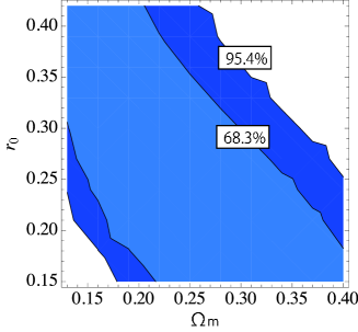
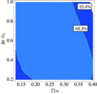
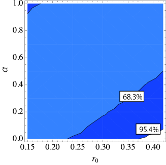
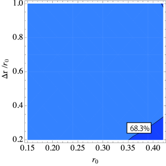
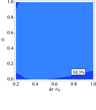
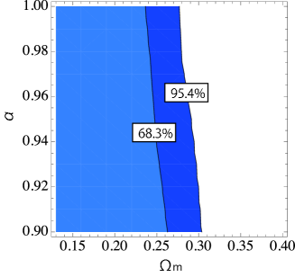
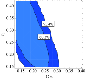
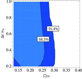
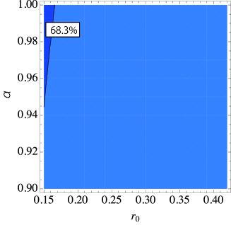
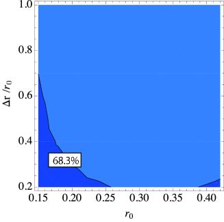
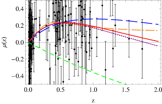
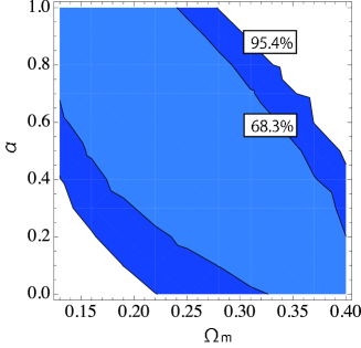
Numerically solving Eq.(39) for lattice points in this region, we sought the smallest $\chi^{2}$ both in whole $\mathcal{V}$ and in the region restricted to $\alpha\geq 0.9$, $\mathcal{V}|_{\alpha\geq 0.9}$. The best-fit parameters giving the smallest $\chi^{2}$ are summarized in Table 1. For comparison, we included the results corresponding to the isotropic void model $(\alpha=1)$. Figures 1 and 2 show confidence regions in selected 2-dim parameter spaces, obtained after integrating over the remaining 2-dim space. (We determined the confidence regions so that the $100\%$ region corresponds to $\mathcal{V}$ or $\mathcal{V}|_{\alpha\geq 0.9}$.) Figure 3 shows residual plots.

Model	Isotropic ($\alpha=1$)	Unbiased ($0.9\leq\alpha$)	Biased ($0\leq\alpha$)
Ratio parameter: $\alpha$	1.0	0.90	$0.42$
Density parameter: $\Omega_{m}$	0.16	0.17	$0.31$
Transition point: $r_{0}$	0.31	0.26	$0.18$
Transition width: $\Delta r/r_{0}$	0.76	0.98	$0.47$
$\chi^{2}$	175.0	174.8	$174.1$

Table 1: The best-fit parameters for the isotropic void model ($\alpha=1$), the unbiased anisotropic model ($0.9\leq\alpha\leq 1.0$), and the possibly biased anisotropic model ($0\leq\alpha\leq 1.0$).

Our best-fit value $\chi^{2}=174.1$ or $174.8$ is smaller than $\chi^{2}_{\Lambda\text{CDM}}=178$ in the $\Lambda\text{CDM}$ model [24] and $\chi^{2}_{\text{void}}=176.5$ in the void model of Alnes et al. [9]. (The value of Alnes et al. is slightly different from our value for $\alpha=1$ shown in Table 1. This is perhaps because they sought the best parameters to fit both SNIa and the first peak of the CMB power spectrum, while we only consider the SNIa.)

The most striking feature of $\alpha$ is that smaller value of this parameter allows larger $\Omega_{m}$ and smaller $r_{0}$ (void size). Linear interpolation of the values in Table 1 gives us the estimate

$$\Omega_{m}=-0.26\alpha+0.42,\quad r_{0}=0.22\alpha+0.09.$$ (58)

The confidence regions shown in Fig.1 also suggest linear relations among these parameters consistent with this estimate, although they do not exactly coincides with the above estimate. This is because the most likely point in the whole parameter space does not necessarily coincide with the most likely point in the reduced parameter space that is obtained by integrating the likelihood function over uninterested (or unfocused) parameters. As a result, the above linear relations do not exactly coincide with the longitudinal lines of the confidence contours in Fig.1. Still, the tendencies are consistent.

This effect of $\alpha$ may be explained as follows. We know that smaller $\alpha$ makes the luminosity distance larger (See Appendix A), while larger $\Omega_{m}$ decreases the distance. Smaller void size also decreases the distance, since our void is defined as an underdense region, where smaller (possibly negative) curvature has an effect of increasing distance. Therefore smaller $\alpha$ can compensate larger $\Omega_{m}$ and smaller void size. Our numerical results seem to confirm this explanation.

The parameter $\Delta r/r_{0}$, which is the boundary width of the void (relative to its radius), appears to be rather insensitive to the likelihood; the confidence regions for $\Delta r/r_{0}$ versus $\Omega_{m}$, $r_{0}$, or $\alpha$ shown in Fig.1 do not provide reasonably sharp prediction about the choice of $\Delta r/r_{0}$. This parameter may therefore be considered less important.

Figure 1: Confidence regions in the space of two parameters obtained from the 4 parameter space $\mathcal{V}$, after integrating over the remaining 2-dim space.

Figure 2: Confidence regions in the space of two parameters obtained from the restricted 4 parameter space $\mathcal{V}|_{\alpha\geq 0.9}$, after integrating over the remaining 2-dim space.

Figure 3: Residual plots of distance modulus for the unbiased best model $(\Omega_{m},r_{0},\Delta r/r_{0},\alpha)=(0.17,0.26,0.98,0.90)$ (red solid line), the biased best model $(0.31,0.18,0.47,0.42)$ (orange chain line), and the $\Lambda$CDM model $(\Omega_{m},\Omega_{\Lambda})=(0.25,0.73)$ (blue longer-interval dashed line) with the base horizontal line being the negative curvature FL model with $(\Omega_{m},\Omega_{k})=(0.27,0.73)$. The purple dotted line, corresponding to $(\Omega_{m},r_{0},\Delta r/r_{0},\alpha)=(0.17,0.26,0.98,1.0)$, which is the same as the unbiased best model except the value of $\alpha$, is included to show how much a smaller $\alpha$ increases the distance. The monotonically decreasing green (shorter-interval) dashed line corresponds to the Einstein-de Sitter model $(\Omega_{m}=1)$. The observational data, represented by dots and (error) bars, are taken from the gold samples of Riess et al.[24].

4 Concluding remarks

Since Type Ia supernovae are observed in various directions in the sky, the distance-redshift relation inferred by a collective data of them should be cosidered as an average over the solid angle. On the other hand, the distance-redshift relation (distance function) $D_{A}(z)$ (or $D_{L}(z)$) for a given direction of sight can be theoretically determined by the distance equation that is equivalent to the optical scalar equation. To obtain an effective equation for the spherically averaged distance function $\bar{D}_{A}(z)$ (or $\bar{D}_{L}(z)$), with which the observed distance-redshift relation can directly be compared, we took an average of the distance equation, and found that the effective equation we want is given by the distance equation for the LTB universe with a Dyer-Roeder-like extension. The function $\alpha(z)$ introduced in our effective equation represents the degree to which the Universe fluctuates from an isotropic configuration. Smaller $\alpha$ generally implies larger fluctuation of matter. Our numerical computations demonstrated that smaller $\alpha$ allows larger $\Omega_{m}$ and smaller void size. This will provide a useful guideline for further investigations of inhomogeneous models.

In our numerical study, we chose the function $\alpha(z)$ to be constant for simplicity, but in reality this function should be a monotonically increasing function such that $\alpha(z)\rightarrow 1(z\rightarrow\infty)$, reflecting the fact that the Universe was sufficiently isotropic (and homogeneous) at the last scattering surface. In this paper we only considered luminosity distance-redshift data of SNIa as obserbational data to compare; for this purpose constant $\alpha$ was sufficient. However, to include other kind of data like CMB power spectrum it is inevitable to have a varying $\alpha$, resulting in more parameters to search. It would still be worth exploring such larger parameter space and compare with all available obserbational data including CMB and that of baryon acoustic oscillation. This is a future work.

Appendix A The original Dyer-Roeder extension

Dyer and Roeder [16, 17] considered a simplified model of the Universe in which the matter is almost concentrated into objects such as galaxies, and the light from a distant object travels through the intergalactic, almost empty space. They assume that the geometry is described by the usual Robertson-Walker metric

$$ds^{2}=-dt^{2}+a(t)^{2}\left[\frac{dr^{2}}{1-Kr^{2}}+r^{2}(d\theta^{2}+\sin^{2}{\theta}d\phi^{2})\right],$$ (59)

where $a(t)$ is the scale factor and $K$ is the curvature index.

Let $(t(\lambda),r(\lambda))$ be a null geodesic coming to an observer, with $\lambda$ being the affine parameter. Then, the geodesic equation for $t(\lambda)$ and the null condition in the FL universe are

$$\frac{d^{2}t}{d\lambda^{2}} =\frac{-a\dot{a}}{1-Kr^{2}}\left(\frac{dr}{d\lambda}\right)^{2}, -\left(\frac{dt}{d\lambda}\right)^{2}+\frac{a^{2}}{1-Kr^{2}}\left(\frac{dr}{d\lambda}\right)^{2} =0,$$ (60)

respectively. Using these equations, Eq.(13) yields

$$\frac{d}{d\lambda} =\frac{1}{\omega(0)}\frac{\dot{a}}{a}\left(\frac{dt}{d\lambda}\right)^{2}\frac{d}{dz}$$

$$=\omega(0)\frac{\dot{a}}{a}(1+z)^{2}\frac{d}{dz}$$

$$=\omega(0)H_{\text{FL}}(1+z)^{2}(z)\frac{d}{dz},$$ (61)

where we have used $z=\frac{-1}{\omega(0)}\frac{dt}{d\lambda}-1$ in the second equality, and $H_{\text{FL}}(z)\equiv\dot{a}/a$ is the Habble parameter for the FL universe. With Eq.(61), this yields the distance equation

$$\mathcal{L}_{\text{FL}}D^{(\text{FL})}_{A}(z)+4\pi G\rho_{\text{FL}}(z)D^{(\text{FL})}_{A}(z)=0,$$ (62)

where we have defined

$$\mathcal{L}_{\text{FL}}\equiv H_{\text{FL}}(z)\frac{d}{dz}\left[H_{\text{FL}}(z)(1+z)^{2}\frac{d}{dz}\right],$$ (63)

and $D^{(\text{FL})}_{A}$ is the angular-diameter distance in the FL universe and $\rho_{\text{FL}}$ the matter density.

To take into account the effect of lumps, Dyer and Roeder reduced, in the above equation, the matter density $\rho_{\text{FL}}(z)$ on the light path to $\alpha_{\text{DR}}\rho_{\text{FL}}$ by a constant $\alpha_{\text{DR}}(0\leq\alpha_{\text{DR}}\leq 1)$. As a result, the Dyer-Roeder equation is given by

$$\mathcal{L}_{\text{FL}}D^{(\text{DR})}_{A}(z)+4\pi G\alpha_{\text{DR}}\rho_{\text{FL}}(z)D^{(\text{DR})}_{A}(z)=0,$$ (64)

where $D^{(\text{DR})}_{A}(z)$ is the angular-diameter distance in a lumpy universe with parameter $\alpha_{\text{DR}}$. In this equation, the value $\alpha_{\text{DR}}=1$ corresponds to the homogeneous universe, and the value $\alpha_{\text{DR}}=0$ to a universe where all the matter is concentrated into lumps.

If the universe is flat ($K=0$), we can easily solve Eq.(64) under the initial conditions $D^{(\text{DR})}_{A}(0)=0$ and $dD^{(\text{DR})}_{A}(0)/dz=1/H_{0}\equiv 1/H_{\text{FL}}(0)$. The solution is

$$D^{(\text{DR})}_{A}(z) =\frac{2}{H_{0}\sqrt{25-24\alpha_{\text{DR}}}}\left[(1+z)^{-b_{1}}-(1+z)^{-b_{2}}\right],$$ (65)

$$\bigl{(}b_{1} \equiv\frac{5-\sqrt{25-24\alpha_{\text{DR}}}}{4},b_{2}\equiv\frac{5+\sqrt{25-24\alpha_{\text{DR}}}}{4}\bigr{)}.$$ (66)

From Eq.(52), the corresponding luminosity distance is

$$D^{(\text{DR})}_{L}(z)=\frac{2(1+z)^{2}}{H_{0}\sqrt{25-24\alpha_{\text{DR}}}}\left[(1+z)^{-b_{1}}-(1+z)^{-b_{2}}\right].$$ (67)

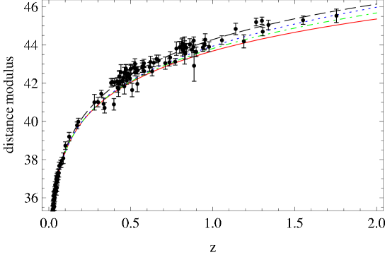
Fig.4 shows the relation between the distance modulus Eq.(55) and the redshift $z$ for various $\alpha_{\text{DR}}$. As seen from these plots, the distance increases when $\alpha<1$ as compared to $\alpha=1$. (Actually we can show that the distance monotonically increases as $\alpha_{\text{DR}}$ decreases, i.e., $\partial D_{A}(z;\alpha_{\text{DR}})/\partial\alpha_{\text{DR}}<0$, for this case.) In other words, the distance takes the maximum at $\alpha_{\text{DR}}=0$, but it still insufficient to explain the observation.

Figure 4: The $\mu$-$z$ relations in the original Dyer-Roeder model with observational data. The solid (red), chain (green), and dotted (blue) lines correspond to $\alpha_{\text{DR}}=1$, $\alpha_{\text{DR}}=0.5$, and $\alpha_{\text{DR}}=0$, respectively. The dashed (black) line corresponds to the $\Lambda$CDM model. The observational data are the gold data[24].

References

• [1] Supernova Search Team, A. G. Riess et al., Astron. J. 116, 1009 (1998), astro-ph/9805201.
• [2] Supernova Cosmology Project, S. Perlmutter et al., Astrophys. J. 517, 565 (1999), astro-ph/9812133.
• [3] E. J. Copeland, M. Sami, and S. Tsujikawa, International Journal of Modern Physics D 15, 1753 (2006).
• [4] C. Marinoni, P. Monaco, G. Giuricin, and B. Costantini, Astrophys. J. 521, 50 (1999); R. O. Marzke, L. N. da Costa, P. S. Pellegrini, C. N. A. Willmer and M. J. Geller, Astrophys. J. 503, 617 (1998); S. Folkes et al., Mon. Not. Roy. Astron. Soc. 308, 459 (1999); E. Zucca et al., A&A 326, 477 (1997).
• [5] M. R. Blanton et al., Astron. J. 121, 2358 (2001), astro-ph/0012085.
• [6] K. Tomita, Astrophys. J. 529, 26 (2000), astro-ph/9905278.
• [7] K. Tomita, Prog. Theor. Phys. 106, 929 (2001), astro-ph/0104141.
• [8] K. Tomita, Mon. Not. Roy. Astron. Soc. 326, 287 (2001), astro-ph/0011484.
• [9] H. Alnes, M. Amarzguioui, and Ø. Grøn, Phys. Rev. D73, 083519 (2006), astro-ph/0512006.
• [10] S. Alexander, T. Biswas, A. Notari and D. Vaid, arXiv:0712.0370 [astro-ph].
• [11] J. Garcia-Bellido and T. Haugboelle, JCAP 0804, 003 (2008), arXiv:0802.1523 [astro-ph].
• [12] G. Lemaître, Ann. Soc. Sci. Bruxelles A 53, 51 (1933).
• [13] R. C. Tolman, Proc. Nat. Acad. Sci. 20, 169 (1934).
• [14] H. Bondi, Mon. Not. Roy. Astron. Soc. 107, 410 (1947).
• [15] C. M. Yoo, T. Kai and K. i. Nakao, Prog. Theor. Phys.  120, 937 (2008) [arXiv:0807.0932 [astro-ph]].
• [16] C. C. Dyer and R. C. Roeder, Astrophys. J. 174, L115 (1972).
• [17] C. C. Dyer and R. C. Roeder, Astrophys. J. 180, L31 (1973).
• [18] T. Mattsson, (2007), arXiv:0711.4264 [astro-ph].
• [19] R. K. Sachs, Proc. Roy. Soc. Lond. A264, 309 (1961).
• [20] R. M. Wald, ”General Relativity”, The University of Chicago Press, Chicago, (1984).
• [21] M. Tanimoto and Y. Nambu, Class. Quant. Grav. 24, 3843 (2007), gr-qc/0703012.
• [22] N. Mustapha, C. Hellaby, and G. F. R. Ellis, Mon. Not. Roy. Astron. Soc. 292, 817 (1997), gr-qc/9808079.
• [23] Y. Wang, D. N. Spergel, and E. L. Turner, Astrophys. J. 498, 1 (1998), astro-ph/9708014.
• [24] Supernova Search Team, A. G. Riess et al., Astrophys. J. 607, 665 (2004), astro-ph/0402512.
• [25] M.-N. Célérier, Astron. Astrophys. 353, 63 (2000), astro-ph/9907206.
• [26] I. M. H. Etherington, Phil. Mag. ser. 7 15, 761 (1933).
• [27] G. F. R. Ellis, in “General Relativity and Cosmology,” Proc. Int. School of Physics “Enrico Fermi”, Course XLVII, ed. R. K. Sachs, Academic Press (1971) 104.