Revision of the fractional exclusion statistics

Abstract

I discuss the concept of fractional exclusion statistics (FES) and I show that in order to preserve the thermodynamic consistency of the formalism, the exclusion statistics parameters should change if the species of particles in the system are divided into subspecies. Using a simple and intuitive model I deduce the general equations that have to be obeyed by the exlcusion statistics parameters in any FES system.

1 Introduction

In Ref. [1] Haldane introduced the fruitful concept of fractional exclusion statistics (FES). Although many authors analyzed the physical properties of FES systems and the microscopic reasons for the manifestation of this type of statistics (see [2, 3, 4, 5, 6, 7, 8, 9, 10, 11, 12, 13, 14, 15] and references therein, just as examples), there are important properties that have been overlooked. In Ref. [16] I proved that if the mutual exclusion statistics parameters (see below the definitions) are defined in the typical way (e.g. like in [1, 2]), then the thermodynamics of the system is inconsistent. To restore the thermodynamics, I conjectured in the same paper that any of the mutual exclusion statistics parameters should be proportional to the dimension of the space on which it acts.

In another paper [17] I showed that FES is manifesting in general in systems of interacting particles and the calculated exclusion statistics parameters have indeed the properties conjectured in [16].

In this letter I analyze the basic properties of the mutual exclusion statistics parameters based on simple, general arguments and I show that the conjectures introduced in [16] are, simply, necessary conditions for the logical consistency of the formalism. This is not surprising, since the inconsistency of the thermodynamics proved in Ref. [16] could have been only a consequence of an unconsistent undelying physical model.

2 A simple model

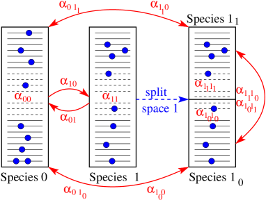
Let us assume that we have a system formed of only two species of particles, 0 and 1, like in Fig. 1. We denote the exclusion statistics parameters of this system by $\tilde{\alpha}_{00},\tilde{\alpha}_{01},\tilde{\alpha}_{10}$ and $\tilde{\alpha}_{11}$, and we start in the standard way [1, 2] by writing the total number of configurations corresponding to $N_{0}$ particles of species 0 and $N_{1}$ particles of species 1 as

$$W_{\{0,1\}}=\prod_{i}^{\{0,1\}}\frac{\left[G_{i}+N_{i}-1-\sum_{j}^{0,1}\tilde{\alpha}_{ij}(N_{j}-\delta_{ij})\right]!}{N_{i}!\left[G_{i}-1-\sum_{j}^{0,1}\tilde{\alpha}_{ij}(N_{j}-\delta_{ij})\right]!},$$ (1)

where $G_{0}$ and $G_{1}$ are the number of single-particle states corresponding to the two species of particles. We recall here that the physical interpretation of the exclusion statistics parameters is that at the variations $\delta N_{0}$ and $\delta N_{1}$ of the particle numbers $N_{0}$ and $N_{1}$, the number of single-particle states available for the two species changes by $\delta G_{0}=-\tilde{\alpha}_{00}\delta N_{0}-\tilde{\alpha}_{01}\delta N_{1}$ and $\delta G_{1}=-\tilde{\alpha}_{10}\delta N_{0}-\tilde{\alpha}_{11}\delta N_{1}$.

If all the $G_{0}$ states have the same energy, say $\epsilon_{0}$, and all the $G_{1}$ states have the energy $\epsilon_{1}$, we may write the grandcanonical partition function of the system as

$${\mathcal{Z}}_{\{0,1\}}=W_{\{0,1\}}\prod_{i}^{\{0,1\}}e^{\beta N_{i}(\mu_{i}-\epsilon_{i})},$$ (2)

where $\beta\equiv(k_{B}T)^{-1}$, $\mu_{0}$ and $\mu_{1}$ are the chemical potentials of the two species of particles, and $T$ is the temperature, common to both species.

To calculate the thermodynamics of the system, we assume that all the numbers involved in our problem are very big, i.e. $N_{0}$, $N_{1}$, $G_{0}-1+\tilde{\alpha}_{00}-\tilde{\alpha}_{00}N_{0}-\tilde{\alpha}_{01}N_{1}$, and $G_{1}-1+\tilde{\alpha}_{11}-\tilde{\alpha}_{10}N_{0}-\tilde{\alpha}_{11}N_{1}$ are much bigger than 1. Maximizing ${\mathcal{Z}}$–by calculating its logarithm and using the Stirling approximation–we obtain the maximum probability populations, which are given by the system of equations [2]

$$(1+w_{0})\left(\frac{w_{0}}{1+w_{0}}\right)^{\tilde{\alpha}_{00}}\left(\frac{w_{1}}{1+w_{1}}\right)^{\tilde{\alpha}_{10}} = e^{\beta(\epsilon_{0}-\mu_{0})}$$ (3a)

$$(1+w_{1})\left(\frac{w_{0}}{1+w_{0}}\right)^{\tilde{\alpha}_{01}}\left(\frac{w_{1}}{1+w_{1}}\right)^{\tilde{\alpha}_{11}} = e^{\beta(\epsilon_{1}-\mu_{1})}$$ (3b)

$$(w_{0}+\tilde{\alpha}_{00})N_{0}+\tilde{\alpha}_{01}N_{1} = G_{0}$$ (3c)

$$\tilde{\alpha}_{10}N_{0}+(w_{1}+\tilde{\alpha}_{11})N_{1} = G_{1}$$ (3d)

Figure 1: (Color online) In the total system, formed of two species of particles, 0 and 1, the species 1 is splited into two sub-species, $1_{0}$ and $1_{1}$. This implies a redefinition of the exclusion statistics parameters, which change from the set $\tilde{\alpha}_{00},\tilde{\alpha}_{01},\tilde{\alpha}_{10},\tilde{\alpha}_{11}$, of the original system, into the set $\tilde{\alpha}_{00}^{\prime},\tilde{\alpha}_{01_{0}},\tilde{\alpha}_{01_{1}},\tilde{\alpha}_{1_{0}0},\tilde{\alpha}_{1_{1}0},\tilde{\alpha}_{1_{0}1_{0}},\tilde{\alpha}_{1_{0}1_{1}},\tilde{\alpha}_{1_{1}1_{0}},\tilde{\alpha}_{1_{1}1_{1}}$, of the system after splitting species 1.

2.1 Changing the number of species

Nevertheless, for large systems like the ones analysed above, we can split any of the two species of particles into subspecies and obtain a thermodynamically equivalent system (I shall prove this below). So let us we split for example species 1 into the subspecies $1_{0}$ and $1_{1}$, of dimensions $G_{1_{0}}$ and $G_{1_{1}}$. In this way we describe the total system as consisting of the species 0, $1_{0}$, and $1_{1}$, of particle numbers $N_{0}$, $N_{1_{0}}$, and $N_{1_{1}}$, in Hilbert spaces of dimensions $G_{0}$, $G_{1_{0}}$, and $G_{1_{1}}$. Obviously,

$$N_{1_{0}}+N_{1_{1}}=N_{1}\qquad{\rm and}\qquad G_{1_{0}}+G_{1_{1}}=G_{1}.$$ (4)

We denote the exclusion statistics parameters of the “new” system like in Fig. 1, namely $\tilde{\alpha}_{00}^{\prime}$, $\tilde{\alpha}_{01_{0}}$, $\tilde{\alpha}_{01_{1}}$, $\tilde{\alpha}_{1_{0}0}$, $\tilde{\alpha}_{1_{1}0}$, $\tilde{\alpha}_{1_{0}1_{0}}$, $\tilde{\alpha}_{1_{0}1_{1}}$, $\tilde{\alpha}_{1_{1}1_{0}}$, $\tilde{\alpha}_{1_{1}1_{1}}$. To obtain the consistency relations for the new exclusion statistics parameters, first we use the fact that the variations $\delta N_{1}$ and $\delta G_{0}$ may be written as $\delta N_{1}=\delta N_{1_{0}}+\delta N_{1_{1}}$ and $\delta G_{0}=-\tilde{\alpha}_{00}\delta N_{0}-\tilde{\alpha}_{01}\delta N_{1}=-\tilde{\alpha}^{\prime}_{00}\delta N_{0}-\tilde{\alpha}_{01_{0}}\delta N_{1_{0}}-\tilde{\alpha}_{01_{1}}\delta N_{1_{1}}$. From these identities we obtain

$$\tilde{\alpha}^{\prime}_{00}=\tilde{\alpha}_{00},$$ (5a)

$$\tilde{\alpha}_{01}=\tilde{\alpha}_{01_{0}}=\tilde{\alpha}_{01_{1}}$$ (5b)

by setting $$\delta N_{1}=\delta N_{1_{0}}=\delta N_{1_{1}}=0 \delta N_{0}=\delta N_{1_{0}}=0 \delta N_{0}=\delta N_{1_{1}}=0 G_{1} \delta G_{1}=\delta G_{1_{0}}+\delta G_{1_{1}} \delta G_{1}=-\tilde{\alpha}_{10}\delta N_{0}-\tilde{\alpha}_{11}(\delta N_{1_{0}}+\delta N_{1_{1}}) \delta G_{1_{0}}=-\tilde{\alpha}_{1_{0}0}\delta N_{0}-\tilde{\alpha}_{1_{0}1_{0}}\delta N_{1_{0}}-\tilde{\alpha}_{1_{0}1_{1}}\delta N_{1_{1}} \delta G_{1_{1}}=-\tilde{\alpha}_{1_{1}0}\delta N_{0}-\tilde{\alpha}_{1_{1}1_{0}}\delta N_{1_{0}}-\tilde{\alpha}_{1_{1}1_{1}}\delta N_{1_{1}}$$, or . Then, writing the variation of as , and using the general expressions , , and , we obtain

$$\tilde{\alpha}_{10}=\tilde{\alpha}_{1_{0}0}+\tilde{\alpha}_{1_{1}0}$$ (5c)

$$\tilde{\alpha}_{11}=\tilde{\alpha}_{1_{0}1_{0}}+\tilde{\alpha}_{1_{1}1_{0}}=\tilde{\alpha}_{1_{0}1_{1}}+\tilde{\alpha}_{1_{1}1_{1}}$$ (5d)

by setting the independent fluctuations $\delta N_{0}$, $\delta N_{1_{0}}$, and $\delta N_{1_{1}}$ to zero in proper order.

Now we write the total number of configurations in the system, considering species $1_{0}$ and $1_{1}$ as distinct,

$$W_{\{0,1_{0},1_{1}\}}=\prod_{i}^{\{0,1_{0},1_{1}\}}\frac{\left[G_{i}+N_{i}-1-\sum_{j}^{\{0,1_{0},1_{1}\}}\tilde{\alpha}_{ij}(N_{j}-\delta_{ij})\right]!}{N_{i}!\left[G_{i}-1-\sum_{j}^{\{0,1_{0},1_{1}\}}\tilde{\alpha}_{ij}(N_{j}-\delta_{ij})\right]!},$$ (6)

and we compare $\log W_{\{0,1\}}$ and $\log W_{\{0,1_{0},1_{1}\}}$, within the approximation of large numbers.

After some obvious simplifications, we obtain

$$\log W_{\{0,1\}} = (F_{0}+N_{0})\log(F_{0}+N_{0})+(F_{1}+N_{1})$$ (7a)

$$\times\log(F_{1}+N_{1})-F_{0}\log F_{0}-F_{1}\log F_{1}$$

$$-N_{0}\log N_{0}-N_{1}\log N_{1},$$

$$\log W_{\{0,1_{0},1_{1}\}} = (F^{\prime}_{0}+N_{0})\log(F^{\prime}_{0}+N_{0})+(F_{1_{0}}+N_{1_{0}})$$ (7b)

$$\times\log(F_{1_{0}}+N_{1_{0}})+(F_{1_{1}}+N_{1_{1}})$$

$$\times\log(F_{1_{1}}+N_{1_{1}})-F^{\prime}_{0}\log F^{\prime}_{0}-F_{1_{0}}\log F_{1_{0}}$$

$$-F_{1_{1}}\log F_{1_{1}}-N_{0}\log N_{0}-N_{1}\log N_{1},$$

with

$$F_{0} = G_{0}+N_{0}-1+\tilde{\alpha}_{00}-\tilde{\alpha}_{00}N_{0}-\tilde{\alpha}_{01}N_{1}$$ (8a)

$$F_{1} = G_{1}+N_{1}-1+\tilde{\alpha}_{11}-\tilde{\alpha}_{10}N_{0}-\tilde{\alpha}_{11}N_{1}$$ (8b)

$$F^{\prime}_{0} = G_{0}+N_{0}-1+\tilde{\alpha}_{00}-\tilde{\alpha}_{00}N_{0}-\tilde{\alpha}_{01_{0}}N_{1_{0}}$$ (8c)

$$-\tilde{\alpha}_{01_{1}}N_{1_{1}}$$

$$F_{1_{0}} = G_{1_{0}}+N_{1_{0}}-1+\tilde{\alpha}_{1_{0}1_{0}}-\tilde{\alpha}_{1_{0}0}N_{0}-\tilde{\alpha}_{1_{0}1_{0}}N_{1_{0}}$$ (8d)

$$-\tilde{\alpha}_{1_{0}1_{1}}N_{1_{1}}$$

$$F_{1_{1}} = G_{1_{1}}+N_{1_{1}}-1+\tilde{\alpha}_{1_{1}1_{1}}-\tilde{\alpha}_{1_{1}0}N_{0}-\tilde{\alpha}_{1_{1}1_{0}}N_{1_{0}}$$ (8e)

$$-\tilde{\alpha}_{1_{1}1_{1}}N_{1_{1}}$$

But using Eqs. (4) and (5), one can easily show that

$$F_{0}=F^{\prime}_{0}\ {\rm and}\ F_{1_{0}}+F_{1_{1}}=F_{1}-1+\tilde{\alpha}_{1_{0}1_{0}}+\tilde{\alpha}_{1_{1}1_{1}}-\tilde{\alpha}_{11}\approx F_{1}.$$ (9)

Now notice that if $M$ is a big number and $c$ is a number betweem 0 and 1, then

$$\frac{M\log M-cM\log cM-(1-c)M\log[(1-c)M]}{M\log M}$$

$$=-c\frac{\log c}{\log M}-(1-c)\frac{\log(1-c)}{\log M}$$

$$={\mathcal{O}}(\log^{-1}M)\ll 1.$$ (10)

Therefore from Eqs. (9) and (10) we obtain that

$$\frac{\log W_{\{0,1\}}-\log W_{\{0,1_{0},1_{1}\}}}{\log W_{\{0,1\}}}={\mathcal{O}}(\log^{-1}N)\ll 1,$$ (11)

where $N$ is a number comparable to $N_{0}$ and $N_{1}$. So indeed, as mentioned in the beginning of this subsection, in the limit of large numbers the splitting of the systems species into sub-species does not change the thermodynamics of the system, provided that the consistency conditions (5) are imposed on the $\alpha$s.

Now let us compare the equilibrium distributions of particles in the two descriptions of the system. If we maxmize the partition function ${\mathcal{Z}}_{\{0,1_{0},1_{1}\}}=W_{\{0,1_{0},1_{1}\}}\prod_{i}^{\{0,1_{0},1_{1}\}}e^{\beta N_{i}(\mu_{i}-\epsilon_{i})}$, with respect to the populations we obtain the new system of equations

$$e^{\beta(\epsilon_{0}-\mu_{0})} = (1+w^{\prime}_{0})\left(\frac{w^{\prime}_{0}}{1+w^{\prime}_{0}}\right)^{\tilde{\alpha}_{00}}\left(\frac{w_{1_{0}}}{1+w_{1_{0}}}\right)^{\tilde{\alpha}_{1_{0}0}}$$ (12a)

$$\times\left(\frac{w_{1_{1}}}{1+w_{1_{1}}}\right)^{\tilde{\alpha}_{1_{1}0}}$$

$$e^{\beta(\epsilon_{1}-\mu_{1})} = (1+w_{1_{0}})\left(\frac{w^{\prime}_{0}}{1+w^{\prime}_{0}}\right)^{\tilde{\alpha}_{01}}\left(\frac{w_{1_{0}}}{1+w_{1_{0}}}\right)^{\tilde{\alpha}_{1_{0}1_{0}}}$$ (12b)

$$\times\left(\frac{w_{1_{1}}}{1+w_{1_{1}}}\right)^{\tilde{\alpha}_{1_{1}1_{0}}}$$

$$e^{\beta(\epsilon_{1}-\mu_{1})} = (1+w_{1_{1}})\left(\frac{w^{\prime}_{0}}{1+w^{\prime}_{0}}\right)^{\tilde{\alpha}_{01}}\left(\frac{w_{1_{0}}}{1+w_{1_{0}}}\right)^{\tilde{\alpha}_{1_{0}1_{1}}}$$ (12c)

$$\times\left(\frac{w_{1_{1}}}{1+w_{1_{1}}}\right)^{\tilde{\alpha}_{1_{1}1_{1}}}$$

$$G_{0} = w^{\prime}_{0}N_{0}+\tilde{\alpha}^{\prime}_{00}N_{0}+\tilde{\alpha}_{01_{0}}N_{1_{0}}+\tilde{\alpha}_{01_{1}}N_{1_{1}}$$ (12d)

$$G_{1_{0}} = w_{1_{0}}N_{1_{0}}+\tilde{\alpha}_{1_{0}0}N_{0}+\tilde{\alpha}_{1_{0}1_{0}}N_{1_{0}}+\tilde{\alpha}_{1_{0}1_{1}}N_{1_{1}}$$ (12e)

$$G_{1_{1}} = w_{1_{1}}N_{1_{1}}+\tilde{\alpha}_{1_{1}0}N_{0}+\tilde{\alpha}_{1_{1}1_{0}}N_{1_{0}}+\tilde{\alpha}_{1_{1}1_{1}}N_{1_{1}}$$ (12f)

where we used the notation $w^{\prime}_{0}$, to distinguish the solutions of the system (12) from the solutions of the system (3). Using the conditions (5), we can compare the two sets of solutions.

We start with Eq. (12d) in which we plug Eqs. (5a), (5b), and (4); we obtain $(w^{\prime}_{0}+\tilde{\alpha}_{00})N_{0}+\tilde{\alpha}_{01}N_{1}=G_{0}$, so we can conclude, after inspecting Eq. (3c), that

$$w^{\prime}_{0}=w_{0}.$$ (13a)

To obtain a relation between $$w_{1} w_{1_{0}} w_{1_{1}} G_{1}=\tilde{\alpha}_{10}N_{0}+(w_{1_{1}}+\tilde{\alpha}_{11})N_{1}+(w_{1_{0}}-w_{1_{1}})N_{1_{0}} N_{1_{0}}<N_{1}$$, , and , we add Eqs. (12e) and (12f). After some simple algebraic manipulations, using Eqs. (5) and (4), we obtain , which should hold for arbitrary . Comparing this result with Eq. (3d) we conclude that

$$w_{1}=w_{1_{0}}=w_{1_{1}}$$ (13b)

Using now Eqs. (5) and (13) we observe that Eqs. (12a), (12b), and (12c) are reduced to the Eqs. (3a) and (3a), so the systems of equations (3) and (12) are indeed equivalent.

Therefore if FES is manifesting into a system, the only physically consistent way of defining it is to impose on its exclusion statistics parameters the conditions (5).

3 The generalization of the simple model

We can extend the model of the previous section to a system of arbitrary number of particle species. We denote now by $N_{i}$ and $G_{i}$ the particle number and the dimension of the single-particle space that contain the species $i$, with $i=0,1,\ldots$. If we split any of the species, say species $j$, into a number of sub-species, $j_{0},j_{1},\ldots$, then all the parameters $\tilde{\alpha}_{kl}$, with both, $k$ and $l$ different from $j$, remain unchanged, whereas the rest of the parameters must satisfy the relations

$$\tilde{\alpha}_{ij} = \tilde{\alpha}_{ij_{0}}=\tilde{\alpha}_{ij_{1}}=\ldots,\ {\rm for\ any}\ i,\ i\neq j$$ (14a)

$$\tilde{\alpha}_{ji} = \tilde{\alpha}_{j_{0}i}+\tilde{\alpha}_{j_{1}i}+\ldots,\ {\rm for\ any}\ i,\ i\neq j$$ (14b)

$$\tilde{\alpha}_{jj} = \tilde{\alpha}_{j_{0}j_{0}}+\tilde{\alpha}_{j_{1}j_{0}}+\ldots$$ (14c)

$$= \tilde{\alpha}_{j_{0}j_{1}}+\tilde{\alpha}_{j_{1}j_{1}}+\ldots=\ldots$$

3.1 The “extensivity” of the mutual exclusion statistics parameters

Notice that the property (14b) of the mutual exclusion statistics parameters is satisfied for a given pair of species, $i$ and $j$, $i\neq j$, if $\tilde{\alpha}_{ji}$ satisfy the relation

$$\tilde{\alpha}_{ji}/G_{j}=\tilde{\alpha}_{j_{0}i}/G_{j_{0}}=\tilde{\alpha}_{j_{1}i}/G_{j_{1}}=\ldots=\alpha_{ji},$$ (15)

for any division of the space $G_{j}$, where $\alpha_{ij}$ is a constant for the pair $(i,j)$. In such a situation $\tilde{\alpha}_{ji}$ is proportional to the dimension of the space on which it acts–$G_{j}$ and $G_{j_{i}}$ in Eq. (15); we say $\tilde{\alpha}_{ji}$ “extensive” [16].

Let us assume that for a given system, we can find a fine enough division into species, such that the extensivity condition (15) is satisfied. Therefore we can write

$$\tilde{\alpha}_{ij}=G_{i}\alpha_{ij},$$ (16)

and we apply the general formalism introduced in Ref. [16]. The populations of the single-particle levels are given by the set of equations

$$\beta(\mu_{i}-\epsilon_{i})+\ln\frac{[1+n_{i}]^{1-\alpha_{ii}}}{n_{i}}=\sum_{j(\neq i)}G_{V_{j}}\ln[1+n_{j}]\alpha_{ji}$$ (17)

where $\mu_{i}$ and $\epsilon_{i}$, are the chemical potential and the energy level of species $i$ ($i=0,1,\ldots$).

Some care should be taken with Eq. (17), since species $i$ of the l.h.s may be divided into sub-species and this would modify both sides of the equation. Therefore Eq. (17) is applicable without any ambiguities in the limit in which the subspecies $i$ is sufficiently small, so that further division would not modify the equation significantly. Nevertheless, in the thermodynamic (quasi-continuous) limit the summations are transformed into integrals and we obtain the integral equation

$$\beta(\mu_{i}-\epsilon_{i})+\ln\frac{[1+n_{i}]^{1-\alpha_{ii}}}{n_{i}}=\int\sigma_{j}\ln[1+n_{j}]\alpha_{jj}\,dj.$$ (18)

where all ambiguities are removed.

4 Conclusions

In this letter I deduced the general conditions necessary for the consistency of the fractional exclusion statistics (FES) formalism. In accordance with Refs. [16, 17, 18], I showed that the exclusion statistics parameters, $\alpha_{ij}$, are not constants, but they change with the species of particles in the system. The consistency conditions on $\alpha$s are given as Eqs. (14).

A particular case for which Eqs. (14) are satisfied is when the mutual exclusion statistics parameters are proportional to the dimension of the space on which they act (see Eq. 15), as conjectured in Ref. [16]. One can eventually find in a physical system a fine enough coarse-graining for which Eq. (15) is satisfied; in such a case the most probable particle ocupation numbers are given by Eqs. (17) or (18).

In Ref. [17] I showed that general systems of interacting particles may be described as ideal systems with FES. The exclusion statistics parameters were calculated and it was proven that the mutual parameters obey Eq. (15) mentioned above.