Sharp kernel clustering algorithms and their associated Grothendieck inequalities

Abstract

In the kernel clustering problem we are given a (large) $n\times n$ symmetric positive semidefinite matrix $A=(a_{ij})$ with $\sum_{i=1}^{n}\sum_{j=1}^{n}a_{ij}=0$ and a (small) $k\times k$ symmetric positive semidefinite matrix $B=(b_{ij})$. The goal is to find a partition $\{S_{1},\ldots,S_{k}\}$ of $\{1,\ldots n\}$ which maximizes $\sum_{i=1}^{k}\sum_{j=1}^{k}\left(\sum_{(p,q)\in S_{i}\times S_{j}}a_{pq}\right)b_{ij}$. We design a polynomial time approximation algorithm that achieves an approximation ratio of $\frac{R(B)^{2}}{C(B)}$, where $R(B)$ and $C(B)$ are geometric parameters that depend only on the matrix $B$, defined as follows: if $b_{ij}=\langle v_{i},v_{j}\rangle$ is the Gram matrix representation of $B$ for some $v_{1},\ldots,v_{k}\in\mathbb{R}^{k}$ then $R(B)$ is the minimum radius of a Euclidean ball containing the points $\{v_{1},\ldots,v_{k}\}$. The parameter $C(B)$ is defined as the maximum over all measurable partitions $\{A_{1},\ldots,A_{k}\}$ of $\mathbb{R}^{k-1}$ of the quantity $\sum_{i=1}^{k}\sum_{j=1}^{k}b_{ij}\langle z_{i},z_{j}\rangle$, where for $i\in\{1,\ldots,k\}$ the vector $z_{i}\in\mathbb{R}^{k-1}$ is the Gaussian moment of $A_{i}$, i.e., $z_{i}=\frac{1}{(2\pi)^{(k-1)/2}}\int_{A_{i}}xe^{-\|x\|_{2}^{2}/2}dx$. We also show that for every $\varepsilon>0$, achieving an approximation guarantee of $(1-\varepsilon)\frac{R(B)^{2}}{C(B)}$ is Unique Games hard.

1 Introduction

Kernel Clustering [13] is a combinatorial optimization problem which originates in the theory of machine learning. It is a general framework for clustering massive statistical data so as to uncover a certain hypothesized structure. The problem is defined as follows: let $A=(a_{ij})$ be an $n\times n$ symmetric positive semidefinite matrix which is usually normalized to be centered, i.e., $\sum_{i=1}^{n}\sum_{j=1}^{n}a_{ij}=0$. The matrix $A$ is often thought of as the correlation matrix of random variables $(X_{1},\ldots,X_{n})$ that measure attributes of certain empirical data, i.e., $a_{ij}=\mathbb{E}\left[X_{i}X_{j}\right]$. We are also given another symmetric positive semidefinite $k\times k$ matrix $B=(b_{ij})$ which functions as a hypothesis, or test matrix. Think of $n$ as huge and $k$ as small. The goal is to cluster $A$ so as to obtain a smaller matrix which most resembles $B$. Formally, we wish to find a partition $\{S_{1},\ldots,S_{k}\}$ of $\{1,\ldots,n\}$ so that if we write $c_{ij}\coloneqq\sum_{(p,q)\in S_{i}\times S_{j}}a_{pq}$, i.e., we form a $k\times k$ matrix $C=(c_{ij})$ by clustering $A$ according to the given partition, then the resulting clustered version of $A$ has the maximum correlation $\sum_{i=1}^{k}\sum_{j=1}^{k}c_{ij}b_{ij}$ with the hypothesis matrix $B$. Equivalently, the goal is to evaluate the number:

$$\mathrm{\bf Clust}(A|B)\coloneqq\max_{\sigma:\{1,\ldots,n\}\to\{1,\ldots,k\}}\sum_{i=1}^{k}\sum_{j=1}^{k}a_{ij}b_{\sigma(i)\sigma(j)}.$$ (1)

The strength of this generic clustering framework is based in part on the flexibility of adapting the matrix $B$ to the problem at hand. Various particular choices of $B$ lead to well studied optimization problems, while other specialized choices of $B$ are based on statistical hypotheses which have been applied with some empirical success. We refer to [13, 7] for additional background and a discussion of specific examples.

In [7] we investigated the computational complexity of the kernel clustering problem. Answering a question posed in [13], we showed that this problem has a constant factor polynomial time approximation algorithm. We refer to [7] for more information on the best known approximation guarantees. We also obtained hardness results for kernel clustering under various complexity assumptions. For example, we showed in [7] that when $B=I_{3}$ is the $3\times 3$ identity matrix then a $\frac{16\pi}{27}$ approximation guarantee for $\mathrm{\bf Clust}(A|I_{3})$ is achievable, while any approximation guarantee smaller than $\frac{16\pi}{27}$ is Unique Games hard. We will discuss the Unique Games Conjecture (UGC) presently. At this point it suffices to say that the above statement is evidence that the hardness threshold of the problem of approximating $\mathrm{\bf Clust}(A|I_{3})$ is $\frac{16\pi}{27}$, or more modestly that obtaining a polynomial time algorithm which approximates $\mathrm{\bf Clust}(A|I_{3})$ up to a factor smaller than $\frac{16\pi}{27}$ would require a major breakthrough.

Another result proved in [7] is that when $k\geq 3$ and $B$ is either the $k\times k$ identity matrix or is spherical (i.e., $b_{ii}=1$ for all $i\in\{1,\ldots,k\}$) and centered (i.e., $\sum_{i=1}^{k}\sum_{j=1}^{k}b_{ij}=0$) then there is a polynomial time approximation algorithm which, given $A$, approximates $\mathrm{\bf Clust}(A|B)$ to within a factor of $\frac{8\pi}{9}\left(1-\frac{1}{k}\right)$. We also presented in [7] a conjecture (called the Propeller Conjecture) which we proved would imply that $\frac{8\pi}{9}\left(1-\frac{1}{k}\right)$ is the UGC hardness threshold when $B=I_{k}$. We refer to [7] for more information on the Propeller Conjecture, which at present remains open.

The above quoted result from [7] settles the problem of evaluating the UGC hardness threshold of the following type of algorithmic task: given $A$ and an hypothesis matrix $B$ which is guaranteed to belong to a certain class of matrices (in our case centered and spherical), approximate efficiently the number $\mathrm{\bf Clust}(A|B)$. Naturally this can be refined to a family of optimization problems which depend on a fixed $B$: for each $B$, what is the UGC hardness threshold of the problem of, given $A$, approximating $\mathrm{\bf Clust}(A|B)$? In [7] we answered this question only when $B=I_{3}$, and for $B=I_{k}$ assuming the Propeller Conjecture, and asked about the case of general $B$ (we did give some $B$-dependent bounds in [7], but they were not sharp for $B\neq I_{k}$ for reasons that will become clear presently). This is a natural question since it makes sense to use the best possible polynomial time algorithm if we know $B$ in advance.

Here we answer the above question in full generality. To explain our results we need to define two geometric parameters which are associated to $B$. Since $B$ is symmetric and positive semidefinite we can find vectors $v_{1},\ldots,v_{k}\in\mathbb{R}^{k}$ such that $B$ is their Gram matrix, i.e., $b_{ij}=\langle v_{i},v_{j}\rangle$ for all $i,j\in\{1,\ldots,k\}$. Let $R(B)$ be the smallest possible radius of a Euclidean ball in $\mathbb{R}^{k}$ which contains $\{v_{1},\ldots,v_{k}\}$ and let $w(B)$ be the center of this ball. Let $C(B)$ be the maximum over all partitions $\{A_{1},\ldots,A_{k}\}$ of $\mathbb{R}^{k-1}$ into measurable sets of the quantity $\sum_{i=1}^{k}\sum_{j=1}^{k}b_{ij}\langle z_{i},z_{j}\rangle$, where for $i\in\{1,\ldots,k\}$ the vector $z_{i}\in\mathbb{R}^{k-1}$ is the Gaussian moment of $A_{i}$, i.e., $z_{i}=\frac{1}{(2\pi)^{(k-1)/2}}\int_{A_{i}}xe^{-\|x\|_{2}^{2}/2}dx$ (this maximum exists, as shown in Section 2). Our main result is the following theorem:

Theorem 1.1.

For every symmetric positive semidefinite $k\times k$ matrix $B$ there exists a randomized polynomial time algorithm which given an $n\times n$ symmetric positive semidefinite centered matrix $A$, outputs a number $\mathrm{Alg}(A)$ such that

$$\mathrm{\bf Clust}(A|B)\leq\mathbb{E}\left[\mathrm{Alg}(A)\right]\leq\frac{R(B)^{2}}{C(B)}\mathrm{\bf Clust}(A|B).$$

On the other hand, assuming the Unique Games Conjecture, no polynomial time algorithm approximates $\mathrm{\bf Clust}(A|B)$ to within a factor strictly smaller than $\frac{R(B)^{2}}{C(B)}$.

As an example of Theorem 1.1 for a particular hypothesis matrix consider the following perturbation of the previously studied case $B=I_{3}$:

$$B_{c}\coloneqq\begin{pmatrix}1&0&0\\ 0&1&0\\ 0&0&c\end{pmatrix},$$

where $c>0$ is a parameter. The problem of approximating efficiently $\mathrm{\bf Clust}(A|B_{c})$ corresponds to partitioning the rows of $A$ into $3$ sets $S_{1},S_{2},S_{3}\subseteq\{1,\ldots,n\}$ and maximizing the sum of the total masses of $A$ on $S_{1}\times S_{1},S_{2}\times S_{2},S_{3}\times S_{3}$, where the parameter $c$ can be used to tune the weight of the set $S_{3}$. This problem is not particularly important—we chose it just as a concrete example for the sake of illustration. In Section 6 we compute the parameters $R(B_{c}),C(B_{c})$ and deduce that the UGC hardness threshold of the problem of computing $\mathrm{\bf Clust}(A|B_{c})$ equals $\frac{4\pi c(1+c)^{2}}{(1+2c)^{3}}$ if $c\geq\frac{1}{2}$ and equals $\frac{\pi(1+c)^{2}}{2+4c}$ if $c\leq\frac{1}{2}$. The change at $c=\frac{1}{2}$ corresponds in a qualitative change in the best algorithm for computing $\mathrm{\bf Clust}(A|B_{c})$—we refer to Section 6 for an explanation.

In the remainder of this introduction we will explain the various ingredients of Theorem 1.1 (in particular the Unique Games Conjecture), and the new ideas used in its proof.

The main tool in the design of the algorithm in Theorem 1.1 is a natural generalization of the positive semidefinite Grothendieck inequality. In [4] Grothendieck proved that there exists a universal constant $K>0$ such that for every $n\times n$ symmetric positive semidefinite matrix $A=(a_{ij})$ we have:

$$\max_{x_{1},\ldots,x_{n}\in S^{n-1}}\sum_{i=1}^{n}\sum_{j=1}^{n}a_{ij}\langle x_{i},x_{j}\rangle\leq K\max_{\varepsilon_{1},\ldots,\varepsilon_{n}\in\{-1,1\}}\sum_{i=1}^{n}\sum_{j=1}^{n}a_{ij}\varepsilon_{i}\varepsilon_{j}.$$ (2)

The best constant $K$ in (2) was shown in [11] to be equal to $\frac{\pi}{2}$. A natural variant of (2) is to replace the numbers $-1,1$ by general $v_{1},\ldots,v_{k}\in\mathbb{R}^{k}$, namely one might ask for the smallest constant $K>0$ such that for every symmetric positive semidefinite $n\times n$ matrix $A$ we have:

$$\max_{x_{1},\ldots,x_{n}\in S^{n-1}}\sum_{i=1}^{n}\sum_{j=1}^{n}a_{ij}\langle x_{i},x_{j}\rangle\leq K\max_{u_{1},\ldots,u_{n}\in\{v_{1},\ldots,v_{k}\}}\sum_{i=1}^{n}\sum_{j=1}^{n}a_{ij}\langle u_{i},u_{j}\rangle.$$ (3)

In Section 3 we prove that (3) holds with $K=\frac{1}{C(B)}$, where $B=\left(\langle v_{i},v_{j}\rangle\right)$ is the Gram matrix of $v_{1},\ldots,v_{k}$, and that this constant is sharp. This inequality is proved along the following lines. Fix $n$ unit vectors $x_{1},\ldots,x_{n}\in S^{n-1}$. Let $G=(g_{ij})$ be a $(k-1)\times n$ random matrix whose entries are i.i.d. standard Gaussian random variables. Let $A_{1},\ldots,A_{k}\ \subseteq\mathbb{R}^{k-1}$ be a measurable partition of $\mathbb{R}^{k-1}$ at which $C(B)$ is attained. Define a random choice of $u_{i}\in\{v_{1},\ldots,v_{k}\}$ by setting $u_{i}=v_{\ell}$ for the unique $\ell\in\{1,\ldots,k\}$ such that $Gx_{i}\in A_{\ell}$. The fact that (3) holds with $K=\frac{1}{C(B)}$ is a consequence of the following fact, which we prove in Section 3:

$$\mathbb{E}\left[\sum_{i=1}^{n}\sum_{j=1}^{n}a_{ij}\langle u_{i},u_{j}\rangle\right]\geq C(B)\sum_{i=1}^{n}\sum_{j=1}^{n}a_{ij}\langle x_{i},x_{j}\rangle.$$ (4)

The crucial point in the proof of (4) is the following identity, proved in Lemma 3.2 as a corollary of the closed-form formula for the Poison kernel of the Hermite polynomials: for every two measurable subsets $E,F\subseteq\mathbb{R}^{k-1}$ and any two unit vectors $x,y\in\mathbb{R}^{n}$, we have

$$\Pr\left[Gx\in E\ \mathrm{and}\ Gy\in F\right]\\ =\gamma_{k-1}(E)\gamma_{k-1}(F)+\langle x,y\rangle\left\langle\int_{E}ud\gamma_{k-1}(u),\int_{F}ud\gamma_{k-1}(u)\right\rangle+\sum_{\ell=2}^{\infty}\left\langle x^{\otimes\ell},y^{\otimes\ell}\right\rangle\sum_{\begin{subarray}{c}s\in(\mathbb{N}\cup\{0\})^{k-1}\\ s_{1}+\cdots+s_{k-1}=\ell\end{subarray}}\alpha_{s}(E)\alpha_{s}(F),$$ (5)

for some real coefficients $\{\alpha_{s}(E)\}_{s\in(\mathbb{N}\cup\{0\})^{k-1}},\{\alpha_{s}(F)\}_{s\in(\mathbb{N}\cup\{0\})^{k-1}}\subseteq\mathbb{R}$. Here $\gamma_{k-1}$ denotes the standard Gaussian measure on $\mathbb{R}^{k-1}$. The product structure of the decomposition (5) hints at the role of the fact that $A$ is positive semidefinite in the proof of (4)—the complete details appear in Section 3.

Once the generalized Grothendieck inequality (18) is obtained with $K=\frac{1}{C(B)}$ it is simple to design the algorithm whose existence is claimed in Theorem 1.1, which is based on semidefinite programming—this is done in Section 4.

We shall now pass to an explanation of the hardness result in Theorem 1.1. The Unique Games Conjecture, posed by Khot in [6], is as follows. A Unique Game is an optimization problem with an instance ${\mathscr{L}}={\mathscr{L}}(G(V,W,E),n,\{\pi_{vw}\}_{(v,w)\in E})$. Here $G(V,W,E)$ is a regular bipartite graph with vertex sets $V$ and $W$ and edge set $E$. Each vertex is supposed to receive a label from the set $\{1,\ldots,n\}$. For every edge $(v,w)\in E$ with $v\in V$ and $w\in W$, there is a given permutation $\pi_{vw}:\{1,\ldots,n\}\to\{1,\ldots,n\}$. A labeling of the Unique Game instance is an assignment $\rho:V\cup W\to\{1,\ldots,n\}$. An edge $(v,w)$ is satisfied by a labeling $\rho$ if and only if $\rho(v)=\pi_{vw}(\rho(w))$. The goal is to find a labeling that maximizes the fraction of edges satisfied (call this maximum ${\rm OPT}({\mathscr{L}}))$. We think of the number of labels $n$ as a constant and the size of the graph $G(V,W,E)$ as the size of the problem instance. The Unique Games Conjecture (UGC) asserts that for arbitrarily small constants $\varepsilon,\delta>0$, there exists a constant $n=n(\varepsilon,\delta)$ such that no polynomial time algorithm can distinguish whether a Unique Games instance ${\mathscr{L}}={\mathscr{L}}(G(V,W,E),n,\{\pi_{vw}\}_{(v,w)\in W})$ satisfies ${\rm OPT}({\mathscr{L}})\leq\delta$ (soundness) or there exists a labeling such that for $1-\varepsilon$ fraction of the vertices $v\in V$ all the edges incident with $v$ are satisfied (completeness). This conjecture is (by now) a commonly used complexity assumption to prove hardness of approximation results. Despite several recent attempts to get better polynomial time approximation algorithms for the Unique Game problem (see the table in [3] for a description of known results), the unique games conjecture still stands.

Our UGC hardness result follows the standard “dictatorship test” approach which is prevalent in PCP based hardness proofs, with a new twist which seems to be of independent interest. Since the kernel clustering problem is concerned with an assignment of one of $k$ labels to each of the rows of the matrix $A$, the natural setting of our hardness proof is a dictatorship test for functions on $\{1,\ldots,k\}^{n}$ taking values in $\{1,\ldots,k\}$ (this was already the case in [7]). The general “philosophy” of such hardness proofs is to associate to every such function a certain numerical parameter called the “objective value” (which is adapted to the optimization problem at hand). The general scheme is to show that for some numbers $a,b>0$, if $f$ depends on only one coordinate (i.e., it is a “dictatorship”) then the objective value of $f$ is at least $a$, while if $f$ does not have any coordinate which is too influential then the objective value of $f$ is at most $b+o(1)$ (the $o(1)$ depends on the notion of having no influential coordinates and its exact form is not important for the purpose of this overview—we refer to Section 5 for details). Once such a result is proved, techniques from the theory of Probabilistically Checkable Proofs can show that under a suitable complexity theoretic assumption (in our case the UGC) no polynomial time algorithm can achieve an approximation factor smaller than $\frac{a}{b}$.

Implicit to the above discussion is an underlying product distribution on $\{1,\ldots,k\}^{n}$ with respect to which we measure the influence of variables. In [7] the case of $B=I_{k}$ was solved using the uniform distribution on $\{1,\ldots,k\}$. It turns out that in order to prove the sharp hardness result in Theorem 1.1 we need to use a non-uniform distribution which depends on the geometry of $B$. Namely, writing $B$ as a Gram matrix $b_{ij}=\langle v_{i},v_{j}\rangle$, recall that $R(B)$ is the radius of the smallest Euclidean ball containing $\{v_{1},\ldots,v_{k}\}$ and $w(B)$ is the center of this ball. A simple separation argument shows that $w(B)$ is in the convex hull of the vectors in $\{v_{1},\ldots,v_{k}\}$ whose distance from $w(B)$ is exactly $R(B)$. Writing $w(B)$ as a convex combination of these points and considering the coefficients of this convex combination results in a probability distribution on $\{1,\ldots,k\}$. In our hardness proof we use the $n$-fold product of (a small perturbation of) this probability distribution as the underlying distribution on $\{1,\ldots,k\}$ for our dictatorship test—see Figure 1 for a schematic description of the situation described above. The full details of this approach, including all the relevant definitions, are presented in Section 5.

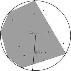
Figure 1: The geometry of the test matrix $B$ induces a dictatorship test: the points above are the vectors $\{v_{1},\ldots,v_{k}\}\subseteq\mathbb{R}^{k}$ such that $B$ is their Gram matrix. The ball depicted above is the smallest Euclidean ball containing $\{v_{1},\ldots,v_{k}\}$, $R(B)$ is its radius and $w(B)$ is its center. Then $w(B)$ is in the convex hull of the points in $\{v_{1},\ldots,v_{k}\}$ which are at distance exactly $R(B)$ from $w(B)$. Writing $w(B)$ as a convex combination of these boundary points yields a distribution over the labels $\{1,\ldots,k\}$. Our dictatorship test corresponds to selecting a point from the $n$-fold power of this probability space and comparing the behavior of a certain “objective value” (defined in equation (31) below), which depends only on the singleton Fourier coefficients, for dictatorships and for functions with low influences.

1.1 Open problems

We end this introduction with a statement of some open problems.

Question 1.

Theorem 1.1 shows that the UGC hardness threshold of the problem of computing $\mathrm{\bf Clust}(A|B)$ for a fixed hypothesis matrix $B$ equals $\frac{R(B)^{2}}{C(B)}$. It is natural to ask if there is also a polynomial time algorithm which outputs a clustering of $A$ whose value is within a factor of $\frac{R(B)^{2}}{C(B)}$ of the optimal clustering. The issue is that our rounding algorithm uses the partition $\{A_{1},\ldots,A_{k}\}$ of $\mathbb{R}^{k-1}$ at which $C(B)$ is attained. In Section 2 we study this optimal partition, and show that it has a relatively simple structure rather than being composed of general measurable sets: it corresponds to cones which are induced by the faces of a simplex. This information allows us to compute efficiently a partition which comes as close as we wish to the optimal partition when $k$ is fixed, or grows slowly with $n$ (to be safe lets just say for the sake of argument that $k\approx\log\log n$ works). We refer to Remark 2.3 for details. We currently do not know if there is polynomial time rounding algorithm when, say, $k\approx\sqrt{n}$. Given $\varepsilon>0$, is there an algorithm which, given $A$ and $B$, computes $\mathrm{\bf Clust}(A|B)$ to within a factor of $(1+\varepsilon)\frac{R(B)^{2}}{C(B)}$, and runs in time which is polynomial in both $n$ and $k$ (and maybe even $1/\varepsilon$)?

Question 2.

We remind the reader that the Propeller Conjecture remains open. This conjecture is about the value of $C(I_{k})$ when $k\geq 4$. It states that the partition at which $C(I_{k})$ is attained is actually much simpler than what one might initially expect: only $3$ of the sets have positive measure and they form a cylinder over a planar $120^{\circ}$ “propeller”. We refer to [7] for a precise formulation and some evidence for the validity of the Propeller Conjecture.

Question 3.

The kernel clustering problem was stated in [13] for matrices $A$ which are centered. This makes sense from the perspective of machine learning, but it seems meaningful to also ask for the UGC hardness threshold of the same problem when $A$ is not assumed to be centered. In the present paper we did not investigate this case at all, and it seems that the exact UGC hardness threshold when $A$ is not necessarily centered is not known for any interesting hypothesis matrix $B$. Note that in [7] we showed that there is a constant factor polynomial time approximation algorithm when $A$ is not necessarily centered: we obtained in [7] an approximation guarantee of $1+\frac{3\pi}{2}$ in this case, but this is probably suboptimal.

2 Preliminaries on the parameter $C(B)$

Let $B=(b_{ij})_{i,j=1}^{k}\in M_{k}(\mathbb{R})$ be a $k\times k$ symmetric positive semidefinite matrix. In what follows we fix $k\geq 2$ and the matrix $B$. We also fix vectors $v_{1},\ldots,v_{k}\in\mathbb{R}^{k}$ for which $b_{ij}=\langle v_{i},v_{j}\rangle$ for all $i,j\in\{1,\ldots,k\}$.

Let $\gamma_{n}$ denote the standard Gaussian measure on $\mathbb{R}^{n}$, i.e., the density of $\gamma_{n}$ is $\frac{1}{(2\pi)^{n/2}}e^{-\|x\|_{2}^{2}/2}$. We denote by $H_{k}$ the Hilbert space $L_{2}(\gamma_{n})\oplus L_{2}(\gamma_{n})\oplus\cdots\oplus L_{2}(\gamma_{n})$ ($k$ times) and we consider the convex subset $\Delta_{k}(\gamma_{n})\subseteq H_{k}$ give by:

$$\Delta_{k}(\gamma_{n})\coloneqq\left\{(f_{1},\ldots,f_{k})\in H_{k}:\ \forall j\in\{1,\ldots,k\}\ f_{j}\geq 0\ \wedge\ \sum_{j=1}^{k}f_{j}=1\right\}.$$ (6)

Define:

$$C(n,B)\coloneqq\sup_{(f_{1},\ldots,f_{k})\in\Delta_{k}(\gamma_{n})}\sum_{i=1}^{k}\sum_{j=1}^{k}b_{ij}\cdot\left\langle\int_{\mathbb{R}^{n}}xf_{i}(x)d\gamma_{n}(x),\int_{\mathbb{R}^{n}}xf_{j}(x)d\gamma_{n}(x)\right\rangle.$$ (7)

The following lemma is a variant of Lemma 3.1 in [7] (but see Remark 2.1 for an explanation of a subtle difference). It simply states that the supremum in (7) is attained at a $k$-tuple of functions which correspond to a partition of $\mathbb{R}^{n}$.

Lemma 2.1.

There exist disjoint measurable sets $A_{1},\ldots,A_{k}\subseteq\mathbb{R}^{n}$ such that $A_{1}\cup A_{2}\cup\cdots\cup A_{k}=\mathbb{R}^{n}$ and

$$\sum_{i=1}^{k}\sum_{j=1}^{k}b_{ij}\cdot\left\langle\int_{A_{j}}xd\gamma_{n}(x),\int_{A_{j}}xd\gamma_{n}(x)\right\rangle=C(n,B).$$

Proof.

Define $\Psi:\Delta_{k}(\gamma_{n})\to\mathbb{R}$ by

$$\Psi(f_{1},\ldots,f_{k})\coloneqq\sum_{i=1}^{k}\sum_{j=1}^{k}b_{ij}\cdot\left\langle\int_{\mathbb{R}^{n}}xf_{i}(x)d\gamma_{n}(x),\int_{\mathbb{R}^{n}}xf_{j}(x)d\gamma_{n}(x)\right\rangle.$$ (8)

We first observe that $\Psi$ is a convex function. Indeed, fix $\lambda\in[0,1]$ and $(f_{1},\ldots,f_{k}),(g_{1},\ldots,g_{k})\in\Delta_{k}(\gamma_{n})$. Denote $z_{i}\coloneqq\int_{\mathbb{R}^{n}}xf_{i}(x)d\gamma_{n}(x)$ and $w_{i}\coloneqq\int_{\mathbb{R}^{n}}xg_{i}(x)d\gamma_{n}(x)$ for every $i\in\{1,\ldots,k\}$. Then:

$$\!\!\!\!\!\!\!\!\!\!\!\!\!\!\!\!\lambda\Psi(f_{1},\ldots,f_{k})+(1-\lambda)\Psi(g_{1},\ldots,g_{k})-\Psi(\lambda f_{1}+(1-\lambda)g_{1},\ldots,\lambda f_{k}+(1-\lambda)g_{k})$$

$$= \sum_{i=1}^{k}\sum_{j=1}^{k}\langle v_{i},v_{j}\rangle\left(\lambda\langle z_{i},z_{j}\rangle+(1-\lambda)\langle w_{i},w_{j}\rangle-\langle\lambda z_{i}+(1-\lambda)w_{i},\lambda z_{j}+(1-\lambda)w_{j}\rangle\right)$$

$$= \lambda(1-\lambda)\sum_{i=1}^{k}\sum_{j=1}^{k}\langle v_{i},v_{j}\rangle\langle z_{i}-w_{i},z_{j}-w_{j}\rangle$$

$$= \lambda(1-\lambda)\left\|\sum_{i=1}^{n}v_{i}\otimes(z_{i}-w_{i})\right\|_{2}^{2}\geq 0.$$

Since $\Delta_{k}(\gamma_{n})$ is a weakly compact subset of $H_{k}$ and $\Psi$ is weakly continuous and convex, $\Psi$ attains its maximum (which equals $C(n,B)$) on $\Delta_{k}(\gamma_{n})$ at an extreme point of $\Delta_{k}(\gamma_{n})$, say at $(f_{1}^{*},\ldots,f_{k}^{*})\in\Delta_{k}(\gamma_{n})$. It follows that there exist measurable sets $A_{1},\ldots,A_{k}\subseteq\mathbb{R}^{n}$ which form a partition of $\mathbb{R}^{n}$ such that $(f_{1}^{*},\ldots,f_{k}^{*})=(\mathbf{1}_{A_{1}},\ldots,\mathbf{1}_{A_{k}})$ almost everywhere, as required.∎

Remark 2.1.

In [7] a stronger result was proved when $B=I_{k}$ (the $k\times k$ identity matrix). Namely, using the notation of the proof of Lemma 2.1 it was shown that the maximum of $\Psi$ on the larger convex set

$$\widetilde{\Delta_{k}(\gamma_{n})}\coloneqq\left\{(f_{1},\ldots,f_{k})\in H_{k}:\ \forall j\in\{1,\ldots,k\}\ f_{j}\geq 0\ \wedge\ \sum_{j=1}^{k}f_{j}\leq 1\right\}$$

is also attained at $(f_{1}^{*},\ldots,f_{k}^{*})=(\mathbf{1}_{A_{1}},\ldots,\mathbf{1}_{A_{k}})$ for some measurable sets $A_{1},\ldots,A_{k}\subseteq\mathbb{R}^{n}$ which form a partition of $\mathbb{R}^{n}$. It turns out that this stronger fact helps to slightly simplify the proof of the corresponding UGC hardness result. However, we do not know how to prove this stronger statement for general $B$, so we formulated the weaker statement in Lemma 2.1, at the cost of needing to modify our proof of the UGC hardness result for general $B$ in Section 5.

The same extreme point argument as in the proof of Lemma 2.1 shows that the maximum of $\Psi$ on $\widetilde{\Delta_{k}(\gamma_{n})}$ is attained at $(f_{1}^{*},\ldots,f_{k}^{*})=(\mathbf{1}_{A_{1}},\ldots,\mathbf{1}_{A_{k}})$ for some disjoint measurable sets $A_{1},\ldots,A_{k}\subseteq\mathbb{R}^{n}$, but now it does not follow that they necessarily cover all of $\mathbb{R}^{n}$. When $B=I_{k}$ it can be shown as in [7] that these sets do cover $\mathbb{R}^{n}$. The same statement is true when $B$ is diagonal, as we now show by arguing as in the proof in [7], but we do not know if it is true for general $B$. So, assume that $B$ is diagonal with positive diagonal entries $(b_{1},\ldots,b_{k})$. Let $A=\mathbb{R}^{n}\setminus\bigcup_{i=1}^{k}A_{k}$. Denote $z_{j}\coloneqq\int_{A_{j}}xd\gamma_{n}(x)$ and $w=\int_{A}xd\gamma_{n}(x)$. Note that $w+z_{1}+\cdots+z_{k}=0$. If $w=0$ then $\Psi$ attains its maximum on the partition $\{A\cup A_{1},A_{2},\ldots,A_{k}\}$, so assume for the sake of contradiction that $w\neq 0$. For every $i\in\{1,\ldots,k\}$ we have:

$$\sum_{j=1}^{n}b_{j}\|z_{j}\|_{2}^{2}=\Psi(\mathbf{1}_{A_{1}},\ldots,\mathbf{1}_{A_{k}})\geq\Psi(\mathbf{1}_{A_{1}},\ldots,\mathbf{1}_{A_{i-1}},\mathbf{1}_{A\cup A_{i}},\mathbf{1}_{A_{i+1}},\ldots,\mathbf{1}_{A_{k}})\\ =\sum_{\begin{subarray}{c}1\leq j\leq k\\ j\neq i\end{subarray}}b_{j}\|z_{j}\|_{2}^{2}+b_{i}\|z_{i}+w\|_{2}^{2}=\sum_{j=1}^{n}b_{j}\|z_{j}\|_{2}^{2}+2b_{i}\langle z_{i},w\rangle+b_{i}\|w\|_{2}^{2}.$$

Thus $2\langle z_{i},w\rangle+\|w\|_{2}^{2}\leq 0$, and if we sum this inequality over $i\in\{1,\ldots,k\}$ while recalling that $w=-\sum_{i=1}^{k}z_{i}$ we see that $(k-2)\|w\|_{2}^{2}\leq 0$, which is a contradiction. Note that for general $B$ the same argument shows that for all $i\in\{1,\ldots,k\}$ we have $2\sum_{j=1}^{k}b_{ij}\left\langle z_{j},w\right\rangle+b_{ii}\|w\|_{2}^{2}\leq 0$. These inequalities do not seem to lend themselves to the same type of easy contradiction as in the case of diagonal matrices. $\lhd$

The proof of the following lemma is an obvious midification of the proof of Lemma 3.2 in [7].

Lemma 2.2.

If $n\geq k-1$ then $C(n,B)=C(k-1,B)$.

Proof.

The inequality $C(n,B)\geq C(k-1,B)$ is easy since for every $(f_{1},\ldots,f_{k})\in\Delta_{k}(\gamma_{k-1})$ we can define $\left(\widetilde{f}_{1},\ldots\widetilde{f}_{k}\right)\in\Delta_{k}(\gamma_{n})$ by $\widetilde{f}_{j}(x,y)=f_{j}(x)$ (thinking here of $\mathbb{R}^{n}$ as $\mathbb{R}^{k-1}\times\mathbb{R}^{n-k+1}$). Then for all $j\in\{1,\ldots,k\}$ we have $\int_{\mathbb{R}^{k-1}}xf_{j}(x)d\gamma_{k-1}(x)=\int_{\mathbb{R}^{n}}x\widetilde{f}_{j}(x)d\gamma_{n}(x)$, implying that $\Psi\left(\widetilde{f}_{1},\ldots\widetilde{f}_{k}\right)=\Psi\left(f_{1},\ldots,f_{k}\right)$.

In the reverse direction, by Lemma 2.1 there is a measurable partition $A_{1},\ldots,A_{k}$ of $\mathbb{R}^{n}$ such that if we define $z_{j}\coloneqq\int_{A_{j}}xd\gamma_{n}(x)\in\mathbb{R}^{n}$ then we have $\sum_{i=1}^{k}\sum_{j=1}^{k}b_{ij}\left\langle z_{i},z_{j}\right\rangle=C(n,B)$. Note that $\sum_{j=1}^{k}z_{j}=0$. Hence the dimension of the subspace $V\coloneqq\mathrm{span}\{z_{1},\ldots,z_{k}\}$ is $d\leq k-1$. Define $g_{1},\ldots,g_{k}:V\to[0,1]$ by $g_{j}(x)=\gamma_{V^{\perp}}\left((A_{j}-x)\cap V^{\perp}\right)$. Then $(g_{1},\ldots,g_{k})\in\Delta_{k}(\gamma_{V})$, so that

$$C(k-1,B) \geq C(d,B)$$

$$\geq \sum_{i=1}^{k}\sum_{j=1}^{k}b_{ij}\left\langle\int_{V}xg_{i}(x)d\gamma_{V}(x),\int_{V}xg_{j}(x)d\gamma_{V}(x)\right\rangle$$

$$= \sum_{i=1}^{k}\sum_{j=1}^{k}b_{ij}\left\langle\int_{V}\int_{V^{\perp}}\mathbf{1}_{A_{i}}(x+y)xd\gamma_{V}(x)d\gamma_{V^{\perp}}(y),\int_{V}\int_{V^{\perp}}\mathbf{1}_{A_{j}}(x+y)xd\gamma_{V}(x)d\gamma_{V^{\perp}}(y)\right\rangle$$

$$= \sum_{i=1}^{k}\sum_{j=1}^{k}b_{ij}\left\langle\int_{A_{i}}\mathrm{Proj}_{V}(w)d\gamma_{n}(w),\int_{A_{j}}\mathrm{Proj}_{V}(w)d\gamma_{n}(w)\right\rangle$$

$$= \sum_{i=1}^{k}\sum_{j=1}^{k}b_{ij}\left\langle\mathrm{Proj}_{V}(z_{i}),\mathrm{Proj}_{V}(z_{j})\right\rangle$$

$$= \sum_{i=1}^{k}\sum_{j=1}^{k}b_{ij}\left\langle z_{i},z_{j}\right\rangle=C(n,B),$$

as required. ∎

In light of Lemma 2.2 we define $C(B)\coloneqq C(k-1,B)$. We shall now prove an analogue of Lemma 3.3 in [7] which gives structural information on the partition $\{A_{1},\ldots,A_{k}\}$ of $\mathbb{R}^{k-1}$ at which $C(B)$ is attained. We first recall some notation and terminology from [7]. Given distinct $z_{1},\ldots,z_{k}\in\mathbb{R}^{k-1}$ and $j\in\{1,\ldots,k\}$ define a set $P_{j}(z_{1},\ldots,z_{k})\subseteq\mathbb{R}^{k}$ by

$$P_{j}(z_{1},\ldots,z_{k})\coloneqq\left\{x\in\mathbb{R}^{k}:\ \langle x,z_{j}\rangle=\max_{i\in\{1,\ldots,k\}}\langle x,z_{i}\rangle\right\}.$$

Thus $\left\{P_{j}(z_{1},\ldots,z_{k})\right\}_{j=1}^{k}$ is a partition of $\mathbb{R}^{k-1}$ which we call the simplicial partition induced by $z_{1},\ldots,z_{k}$ (strictly speaking the elements of this partition are not disjoint, but they intersect at sets of measure $0$).

Lemma 2.3.

Let $A_{1},\ldots,A_{k}\subseteq\mathbb{R}^{k-1}$ be a partition into measurable sets such that if we set $z_{j}\coloneqq\int_{A_{j}}xd\gamma_{k-1}(x)$ then

$$C(B)=\sum_{i=1}^{k}\sum_{j=1}^{k}b_{ij}\left\langle z_{i},z_{j}\right\rangle.$$ (9)

Assume also that this partition is minimal in the sense that the number of elements of positive measure in this partition is minimum among all the possible partitions satisfying (9). Define

$$J\coloneqq\left\{j\in\{1,\ldots,k\}:\ \gamma_{k-1}(A_{j})>0\right\}$$

and set $|J|=\ell$. Then up to an orthogonal transformation $\{z_{j}\}_{j\in J}\subseteq\mathbb{R}^{\ell-1}$ and the vectors $\{z_{j}\}_{j\in J}$ are non-zero and distinct. Moreover, if we define $\{w_{j}\}_{j\in J}\subseteq\mathbb{R}^{\ell-1}$ by

$$w_{j}\coloneqq\sum_{s\in J}b_{js}z_{s},$$ (10)

then the vectors $\{w_{j}\}_{j\in J}$ are distinct and for each $j\in J$ we have

$$A_{j}=P_{j}\big{(}(w_{i})_{i\in J}\big{)}\times\mathbb{R}^{k-\ell}$$ (11)

up to sets of measure zero.

Proof.

Since $\sum_{j\in J}\mathbf{1}_{A_{j}}=1$ almost everywhere we have $\sum_{j\in J}z_{j}=0$. Thus the dimension of the span of $\{z_{j}\}_{j\in J}$ is at most $|J|-1=\ell-1$, and by applying an orthogonal transformation we may assume that $\{z_{j}\}_{j\in J}\subseteq\mathbb{R}^{\ell-1}$. Also, for every distinct $i,j\in J$ replace $A_{i}$ by $A_{i}\cup A_{j}$ and $A_{j}$ by the empty set and obtain a partition of $\mathbb{R}^{k-1}$ which contains exactly $\ell-1$ elements of positive measure and for which we have (by the minimality of $\ell$):

$$C(B) > \sum_{s,t\in J\setminus\{i,j\}}b_{st}\left\langle z_{s},z_{t}\right\rangle+2\sum_{s\in J\setminus\{i,j\}}b_{is}\left\langle z_{s},z_{i}+z_{j}\right\rangle+b_{ii}\left\|z_{i}+z_{j}\right\|_{2}^{2}$$

$$= \sum_{s,t\in J}b_{st}\left\langle z_{s},z_{t}\right\rangle+2\sum_{s\in J}\left(b_{is}-b_{js}\right)\left\langle z_{s},z_{j}\right\rangle+\left(b_{ii}+b_{jj}-2b_{ij}\right)\|z_{j}\|_{2}^{2}$$

$$= C(B)+2\left\langle w_{i}-w_{j},z_{j}\right\rangle+\|v_{i}-v_{j}\|_{2}^{2}\cdot\|z_{j}\|_{2}^{2},$$

where we used the fact that $b_{st}=\left\langle v_{s},v_{t}\right\rangle$. Thus

$$2\left\langle w_{i}-w_{j},z_{j}\right\rangle+\|v_{i}-v_{j}\|_{2}^{2}\cdot\|z_{j}\|_{2}^{2}<0,$$ (12)

and by symmetry we also have the inequality:

$$2\left\langle w_{j}-w_{i},z_{i}\right\rangle+\|v_{i}-v_{j}\|_{2}^{2}\cdot\|z_{i}\|_{2}^{2}<0.$$ (13)

It follows in particular from (12) and (13) that $z_{i}$ and $z_{j}$ are non-zero and that $w_{i}\neq w_{j}$. Moreover if we sum (12) and (13) we get that

$$2\left\langle w_{i}-w_{j},z_{j}-z_{i}\right\rangle+\|v_{i}-v_{j}\|_{2}^{2}\left(\|z_{i}\|_{2}^{2}+\|z_{j}\|_{2}^{2}\right)<0$$

which implies that $z_{i}\neq z_{j}$.

The above reasoning implies in particular that $\left\{P_{j}\big{(}(w_{i})_{i\in J}\big{)}\times\mathbb{R}^{k-\ell}\right\}_{j\in J}$ is a partition of $\mathbb{R}^{k-1}$ (up to pairwise intersections at sets of measure $0$). Assume for the sake of contradiction that these exist $i\in J$ such that

$$\gamma_{k-1}\left(A_{i}\setminus\left(P_{i}\big{(}(w_{s})_{s\in J}\big{)}\times\mathbb{R}^{k-\ell}\right)\right)>0.$$

Arguing as in the proof of Lemma 3.3 in [7] we see that there exists $\varepsilon>0$ and $j\in J\setminus\{i\}$ such that if we denote $E\coloneqq\left\{x\in A_{i}:\ \langle x,z_{j}\rangle\geq\left\langle x,z_{i}\right\rangle+\varepsilon\right\}$ then $\gamma_{k-1}(E)>0$.

Define a partition $\widetilde{A}_{1},\ldots\widetilde{A}_{k}$ of $\mathbb{R}^{k-1}$ by

$$\widetilde{A}_{r}\coloneqq\left\{\begin{array}[]{ll}A_{r}&r\notin\{i,j\}\\ A_{i}\setminus E&r=i\\ A_{j}\cup E&r=j.\end{array}\right.$$

Then for $w\coloneqq\int_{E}xd\gamma_{k-1}(x)$ we have

$$C(B) \geq \sum_{s,t\in J}b_{st}\left\langle\int_{\widetilde{A}_{s}}xd\gamma_{k-1}(x),\int_{\widetilde{A}_{t}}xd\gamma_{k-1}(x)\right\rangle$$

$$= \sum_{s,t\in J\setminus\{i,j\}}b_{st}\left\langle z_{s},z_{t}\right\rangle+2\sum_{s\in J\setminus\{i,j\}}b_{is}\left\langle z_{s},z_{i}-w\right\rangle+2\sum_{s\in J\setminus\{i,j\}}b_{js}\left\langle z_{s},z_{j}+w\right\rangle$$

$$+2b_{ij}\left\langle z_{i}-w,z_{j}+w\right\rangle+b_{ii}\|z_{i}-w\|_{2}^{2}+b_{jj}\|z_{j}+w\|_{2}^{2}$$

$$= C(B)-2\sum_{s\in J}b_{is}\left\langle z_{s},w\right\rangle+2\sum_{s\in J}b_{js}\left\langle z_{s},w\right\rangle+\left(b_{ii}+b_{jj}-2b_{ij}\right)\|w\|_{2}^{2}$$

$$\stackrel{{\scriptstyle\eqref{eq:def w_i}}}{{=}} C(B)+2\left\langle w_{j}-w_{i},w\right\rangle+\|v_{i}-v_{j}\|_{2}^{2}\cdot\|w\|_{2}^{2}$$

$$\geq C(B)+2\int_{E}\left(\langle z_{j},x\rangle-\langle z_{i},x\rangle\right)d\gamma_{k-1}(x)$$

$$\geq C(B)+2\varepsilon\gamma_{k-1}(E)>C(B),$$

a contradiction. ∎

Remark 2.2.

Note that we have the following non-trivial identity as a corollary of Lemma 2.3 (and using the same notation): For each $i\in J$,

$$z_{j}=\int_{P_{j}\big{(}(w_{i})_{i\in J}\big{)}}xd\gamma_{\ell-1}(x),$$ (14)

where we recall that the $w_{i}$ are defined in (10). This system of equalities seems to contain non-trivial information on the structure of the partition at which $C(B)$ is attained. In future research it would be of interest to exploit this information, though we have no need for it for our present purposes.$\lhd$

Remark 2.3.

Given $B$ and $\varepsilon>0$ we can estimate $C(B)$ up to an error of at most $\varepsilon$ in constant time (which depends only on $B,k,\varepsilon$). Moreover, we can compute in constant time a conical simplicial partition of $\mathbb{R}^{k-1}$ at which the value of $\Psi$ is at least $C(B)-\varepsilon$. These statements are a simple corollary of Lemma 2.3. Indeed, all we have to do is to run over all choices of $\ell\in\{1,\ldots,k\}$ and for each such $\ell$ construct an appropriate net of $z_{1},\ldots,z_{\ell}\in\mathbb{R}^{\ell-1}$ of bounded size, and then check each of the induced simplicial partitions of $\mathbb{R}^{k-1}$ as in (11) for the one which maximizes $\Psi$. To this end we need some a priori bound on the length of $z_{i}$: the crude bound

$$\|z_{i}\|_{2}=\left\|\int_{A_{i}}xd\gamma_{\ell-1}(x)\right\|_{2}\leq\int_{\mathbb{R}^{\ell-1}}\|x\|_{2}d\gamma_{\ell-1}(x)\leq\sqrt{\ell}$$

will suffice. Fix $\delta>0$ which will be determined momentarily. Let $\mathcal{N}$ be a $\delta$-net in the Euclidean ball of radius $\sqrt{\ell}$ in $\mathbb{R}^{\ell-1}$. Then $|\mathcal{N}|\leq\left(\frac{3\sqrt{\ell}}{\delta}\right)^{\ell}$.

Let $A_{1},\ldots,A_{k}$ be as in Lemma 2.3, i.e., the true (minimal) partition at which $C(B)$ is attained. Let $J$, $\ell$, $z_{i}$ and $w_{i}$ be as in Lemma 2.3. For each $i\in J$ find $z_{i}^{\prime}\in\mathcal{N}$ for which $\|z_{i}-z_{i}^{\prime}\|_{2}\leq\delta$. Define $w_{i}^{\prime}=\sum_{s\in J}b_{js}z_{s}^{\prime}$. Then we have the crude bound $\|w_{i}-w_{i}^{\prime}\|_{2}\leq\delta\sum_{s=1}^{k}\sum_{t=1}^{k}|b_{st}|\coloneqq\delta\|B\|_{1}$. We also have the a priori bounds $\|w_{i}\|_{2},\|w_{i}^{\prime}\|_{2}\leq\sqrt{\ell}\|B\|_{1}$. By compactness there exists $\delta=\delta(\varepsilon,\ell,B)$ such that these estimates imply that for all $j\in J$,

$$\left\|z_{j}-\int_{P_{j}\big{(}(w_{i}^{\prime})_{i\in J}\big{)}}xd\gamma_{\ell-1}(x)\right\|_{2}=\left\|\int_{P_{j}\big{(}(w_{i})_{i\in J}\big{)}}xd\gamma_{\ell-1}(x)-\int_{P_{j}\big{(}(w_{i}^{\prime})_{i\in J}\big{)}}xd\gamma_{\ell-1}(x)\right\|_{2}\leq\frac{\varepsilon}{2\sqrt{\ell}\|B\|_{1}}.$$ (15)

(It is actually easy to give a concrete bound on the required $\delta$ if so desired, but this is not important for our purposes.) It follows from (15) that:

$$C(B)\geq\sum_{s,t\in J}b_{st}\left\langle\int_{P_{s}\big{(}(w_{i}^{\prime})_{i\in J}\big{)}}xd\gamma_{\ell-1}(x),\int_{P_{t}\big{(}(w_{i}^{\prime})_{i\in J}\big{)}}xd\gamma_{\ell-1}(x)\right\rangle\\ \geq\sum_{s,t\in J}b_{st}\left\langle z_{s},z_{t}\right\rangle-\sum_{s,t\in J}|b_{st}|\cdot\frac{\varepsilon}{2\sqrt{\ell}\|B\|_{1}}\cdot 2\sqrt{\ell}=C(B)-\varepsilon.$$

Note that the above integrals can be estimated efficiently (polynomial time in $k$) with arbitrarily good precision due to the fact that the simplicial cones $P_{j}\big{(}(w_{i}^{\prime})_{i\in J}\big{)}$ have an efficient membership oracle and the Gaussian measure is $\log$-concave. These are very crude bounds that suffice for our algorithmic purposes when $k$ is fixed, but deteriorate exponentially with $k$. It would be of interest to understand whether we can estimate $C(B)$ (and more importantly the associated partitions, as they are used in our rounding procedure) in time which is polynomial in $k$. Perhaps the identities (14) can play a role in the design of such an efficient algorithm, but we did not investigate this issue. $\lhd$

We end this section with a simple analytic interpretation of the parameter $C(B)$. Given a square integrable function $f:\mathbb{R}^{n}\to\mathbb{R}^{k}$ its Rademacher projection $\mathbf{\mathrm{\bf Rad}}(f):\mathbb{R}^{n}\to\mathbb{R}^{k}$ (see [10] for an explanation of this terminology) is defined for $x=(x_{1},\ldots,x_{n})\in\mathbb{R}^{n}$ as:

$$\mathbf{\mathrm{\bf Rad}}(f)(x)=\sum_{i=1}^{n}\left(\int_{\mathbb{R}^{n}}y_{i}f(y)d\gamma_{n}(y)\right)x_{i}.$$

Assume that $f$ takes values in $\{v_{1},\ldots,v_{k}\}\subseteq\mathbb{R}^{k}$ and define $A_{i}=f^{-1}(v_{i})$ for $i\in\{1,\ldots,k\}$. Then $\{A_{1},\ldots,A_{k}\}$ is a measurable partition of $\mathbb{R}^{n}$. We also have the identity:

$$\mathbf{\mathrm{\bf Rad}}(f)(x)=\sum_{i=1}^{n}\left(\sum_{j=1}^{k}v_{j}\int_{A_{j}}y_{i}d\gamma_{n}(y)\right)x_{i}.$$

Thus

$$\left\|\mathbf{\mathrm{\bf Rad}}(f)\right\|_{L_{2}(\gamma_{n},\mathbb{R}^{k})}^{2}=\int_{\mathbb{R}^{n}}\left\|\mathbf{\mathrm{\bf Rad}}(f)(x)\right\|_{2}^{2}d\gamma_{n}(x)=\sum_{i=1}^{n}\left\|\sum_{j=1}^{k}v_{j}\int_{A_{j}}y_{i}d\gamma_{n}(y)\right\|_{2}^{2}\\ =\sum_{i=1}^{n}\sum_{j=1}^{k}\sum_{\ell=1}^{k}\left\langle v_{j},v_{\ell}\right\rangle\left(\int_{A_{j}}y_{i}d\gamma_{n}(y)\right)\left(\int_{A_{\ell}}y_{i}d\gamma_{n}(y)\right)=\sum_{j=1}^{k}\sum_{\ell=1}^{k}b_{j\ell}\left\langle\int_{A_{j}}yd\gamma_{n}(y),\int_{A_{j}}yd\gamma_{n}(y)\right\rangle.$$ (16)

The identity (16) implies the following lemma:

Lemma 2.4.

For every $n\geq k-1$ we have:

$$C(B)=\max_{f:\mathbb{R}^{n}\to\{v_{1},\ldots,v_{k}\}}\left\|\mathbf{\mathrm{\bf Rad}}(f)\right\|_{L_{2}(\gamma_{n},\mathbb{R}^{k})}^{2}.$$

Recall that $R(B)$ is defined as the radius of the smallest ball in $\mathbb{R}^{k}$ which contains the set $\{v_{1},\ldots,v_{k}\}$ and that $w(B)$ is the center of this ball. Lemma 2.4 implies the following corollary:

Corollary 2.5.

$C(B)\leq R(B)^{2}$.

Proof.

Let $\{A_{1},\ldots,A_{k}\}$ be a partition of $\mathbb{R}^{k-1}$ into measurable sets such that if we define $z_{j}=\int_{A_{j}}xd\gamma_{k-1}(x)$ then

$$C(B)=\sum_{i=1}^{k}\sum_{j=1}^{k}\left\langle v_{i},v_{j}\right\rangle\left\langle z_{i},z_{j}\right\rangle\\ =\sum_{i=1}^{k}\sum_{j=1}^{k}\left\langle v_{i}-w(B),v_{j}-w(B)\right\rangle\left\langle z_{i},z_{j}\right\rangle+2\sum_{i=1}^{k}\left\langle v_{i},w(B)\right\rangle\left\langle z_{i},\sum_{j=1}^{k}z_{j}\right\rangle+\|w(B)\|_{2}^{2}\cdot\left\|\sum_{j=1}^{k}z_{j}\right\|_{2}^{2}.$$ (17)

Since $\sum_{j=1}^{k}z_{j}=0$ it follows from (16) and (17) that for $f:\mathbb{R}^{k-1}\to\left\{v_{i}-w(B)\right\}_{i=1}^{k}$ defined by $f|_{A_{i}}=v_{i}-w(B)$ we have:

$$C(B)=\left\|\mathbf{\mathrm{\bf Rad}}(f)\right\|_{L_{2}(\gamma_{n},\mathbb{R}^{k})}^{2}\stackrel{{\scriptstyle(\star)}}{{\leq}}\left\|f\right\|_{L_{2}(\gamma_{n},\mathbb{R}^{k})}^{2}\leq\left\|f\right\|_{L_{\infty}(\gamma_{n},\mathbb{R}^{k})}^{2}=\max_{i\in\{1,\ldots,k\}}\left\|v_{i}-w(B)\right\|_{2}^{2}=R(B)^{2},$$

where in $(\star)$ we used the fact that $\mathbf{\mathrm{\bf Rad}}$ is an orthogonal projection on the Hilbert space $L_{2}(\gamma_{n},\mathbb{R}^{k})$. ∎

3 Generalized positive semidefinite Grothendieck inequalities

The purpose of this section is to prove the following theorem, which as explained in the introduction, is an extension of Grothendieck’s inequality for positive semidefinite matrices.

Theorem 3.1.

Let $A=(a_{ij})\in M_{n}(\mathbb{R})$ be an $n\times n$ symmetric positive semidefinite matrix. Let $v_{1},\ldots,v_{k}\in\mathbb{R}^{k}$ be $k\geq 2$ vectors and let $B=(b_{ij}=\langle v_{i},v_{j}\rangle)$ be the corresponding Gram matrix. Then

$$\max_{x_{1},\ldots,x_{n}\in S^{n-1}}\sum_{i=1}^{n}\sum_{j=1}^{n}a_{ij}\langle x_{i},x_{j}\rangle\leq\frac{1}{C(B)}\max_{\sigma:\{1,\ldots,n\}\to\{1,\ldots,k\}}\sum_{i=1}^{n}\sum_{j=1}^{n}a_{ij}\langle v_{\sigma(i)},v_{\sigma(j)}\rangle.$$ (18)

We shall prove in Section 3.1 that the factor $\frac{1}{C(B)}$ in (18) cannot be improved, even when in (18) $A$ is restricted to be centered, i.e., $\sum_{i=1}^{n}\sum_{j=1}^{n}a_{ij}=0$.

The key tool in the proof of Theorem 3.1 is the following lemma:

Lemma 3.2.

Let $\left\{g_{ij}:\ i\in\{1,\ldots,m\},\ j\in\{1,\ldots,n\}\right\}$ be i.i.d. standard Gaussian random variables and let $G=(g_{ij})$ be the corresponding $m\times n$ random Gaussian matrix. Fix two unit vectors $x,y\in S^{n-1}$ and two measurable subsets $E,F\subseteq\mathbb{R}^{m}$. Then:

$$\Pr\left[Gx\in E\ \wedge\ Gy\in F\right]\\ =\gamma_{m}(E)\gamma_{m}(F)+\langle x,y\rangle\left\langle\int_{E}ud\gamma_{m}(u),\int_{F}ud\gamma_{m}(u)\right\rangle+\sum_{\ell=2}^{\infty}\left\langle x^{\otimes\ell},y^{\otimes\ell}\right\rangle\sum_{\begin{subarray}{c}s\in(\mathbb{N}\cup\{0\})^{m}\\ s_{1}+\cdots+s_{m}=\ell\end{subarray}}\alpha_{s}(E)\alpha_{s}(F),$$ (19)

for some real coefficients $\{\alpha_{s}(E)\}_{s\in(\mathbb{N}\cup\{0\})^{m}},\{\alpha_{s}(F)\}_{s\in(\mathbb{N}\cup\{0\})^{m}}\subseteq\mathbb{R}$.

Proof.

Denote $r=\langle x,y\rangle$. Let $g,h\in\mathbb{R}$ be independent standard Gaussian random variables and let $g_{1},\ldots,g_{m}\in\mathbb{R}^{n}$ be i.i.d. standard Gaussian random vectors in $\mathbb{R}^{n}$ (i.e., they are independent and distributed according to $\gamma_{n}$). Then for each $i\in\{1,\ldots,m\}$ the planar random vector $(\langle g_{i},x\rangle,\langle g_{i},y\rangle)\in\mathbb{R}^{2}$ has the same distribution as $\left(g,rg+\sqrt{1-r^{2}}h\right)\in\mathbb{R}^{2}$, and hence its density is given for $(u,v)\in\mathbb{R}^{2}$ by:

$$f_{r}(u,v)\coloneqq\frac{1}{2\pi\sqrt{1-r^{2}}}\cdot\exp\left(-\frac{u^{2}-2ruv+v^{2}}{2(1-r^{2})}\right).$$

The Hermite polynomials $\{H_{k}\}_{k=0}^{\infty}$ are defined as:

$$H_{k}(t)\coloneqq(-1)^{k}e^{t^{2}}\frac{d^{k}}{dt^{k}}\left(e^{-t^{2}}\right)=\sum_{s=0}^{\lfloor k/2\rfloor}\frac{(-1)^{s}k!}{s!(k-2s)!}(2t)^{k-2s}.$$

The formula for the Poison kernel for Hermite polynomials (see for example equation 6.1.13 in [1] or the discussion in [14]) says that

$$f_{r}(u,v)=\frac{e^{-(u^{2}+v^{2})/2}}{2\pi}\sum_{k=0}^{\infty}\frac{r^{k}}{2^{k}k!}H_{k}\left(\frac{u}{\sqrt{2}}\right)H_{k}\left(\frac{v}{\sqrt{2}}\right).$$

Since the vector $(Gx,Gy)\in\mathbb{R}^{2m}$ has the same distribution as the vector $\big{(}(\langle g_{i},x\rangle,\langle g_{i},y\rangle)\big{)}_{i=1}^{m}$, whose (planar) entries are i.i.d. with density $f_{r}$, we see that:

$$\!\!\!\!\!\!\!\!\!\!\!\!\Pr\left[Gx\in E\ \wedge\ Gy\in F\right]=\int_{E\times F}\left(\prod_{i=1}^{m}f_{r}(u_{i},v_{i})\right)dudv$$

$$= \int_{E\times F}\frac{e^{-(\|u\|_{2}^{2}+\|v\|_{2}^{2})/2}}{(2\pi)^{m}}\left(\prod_{i=1}^{m}\left(\sum_{k=0}^{\infty}\frac{r^{k}}{2^{k}k!}H_{k}\left(\frac{u_{i}}{\sqrt{2}}\right)H_{k}\left(\frac{v_{i}}{\sqrt{2}}\right)\right)\right)dudv$$

$$= \int_{E\times F}\left(\sum_{s\in(\mathbb{N}\cup\{0\})^{m}}\frac{r^{s_{1}+\cdots+s_{m}}}{2^{s_{1}+\cdots+s_{m}}\prod_{i=1}^{m}s_{i}!}\left(\prod_{i=1}^{m}H_{s_{i}}\left(\frac{u_{i}}{\sqrt{2}}\right)\right)\left(\prod_{i=1}^{m}H_{s_{i}}\left(\frac{v_{i}}{\sqrt{2}}\right)\right)\right)d\gamma_{m}(u)d\gamma_{m}(v)$$

$$= \gamma_{m}(E)\gamma_{m}(F)+\langle x,y\rangle\left\langle\int_{E}ud\gamma_{m}(u),\int_{F}ud\gamma_{m}(u)\right\rangle+\sum_{\ell=2}^{\infty}\left\langle x^{\otimes\ell},y^{\otimes\ell}\right\rangle\sum_{\begin{subarray}{c}s\in(\mathbb{N}\cup\{0\})^{m}\\ s_{1}+\cdots+s_{m}=\ell\end{subarray}}\alpha_{s}(E)\alpha_{s}(F),$$

where we used the fact that $H_{0}(t)=1$ and $H_{1}(t)=2t$, and for every measurable subset $W\subseteq R^{m}$ and $s\in(\mathbb{N}\cup\{0\})^{m}$ the notation

$$\alpha_{s}(W)\coloneqq\frac{1}{2^{(s_{1}+\cdots+s_{m})/2}\prod_{i=1}^{m}\sqrt{s_{i}!}}\int_{W}\left(\prod_{i=1}^{m}H_{s_{i}}\left(\frac{u_{i}}{\sqrt{2}}\right)\right)d\gamma_{m}(u).$$

The proof of the identity (14) is complete. ∎

Proof of Theorem 3.1.

Fix $n$ unit vectors $x_{1},\ldots,x_{n}\in S^{n-1}$. Let $\{A_{1},\ldots,A_{k}\}$ be a partition of $\mathbb{R}^{k-1}$ into measurable subsets. Let $G$ be a random Gaussian matrix as in Lemma 3.2 with $m=k-1$. Define a random assignment $\sigma:\{1,\ldots,n\}\to\{1,\ldots,k\}$ by setting $\sigma(i)$ to be the unique $p\in\{1,\ldots,k\}$ for which $Gx_{i}\in A_{p}$. Then for every $i,j\in\{1,\ldots,n\}$ we have

$$\mathbb{E}\left[\left\langle v_{\sigma(i)},v_{\sigma(j)}\right\rangle\right]=\sum_{p=1}^{k}\sum_{q=1}^{k}\left\langle v_{p},v_{q}\right\rangle\Pr\left[Gx_{i}\in A_{p}\ \wedge\ Gx_{j}\in A_{q}\right]=\sum_{p=1}^{k}\sum_{q=1}^{k}b_{pq}\Pr\left[Gx_{i}\in A_{p}\ \wedge\ Gx_{j}\in A_{q}\right].$$

We may therefore apply Lemma 3.2 to deduce that:

$$\mathbb{E}\left[\sum_{i=1}^{n}\sum_{j=1}^{n}a_{ij}\left\langle v_{\sigma(i)},v_{\sigma(j)}\right\rangle\right] = \left(\sum_{i=1}^{n}\sum_{j=1}^{n}a_{ij}\right)\sum_{p=1}^{k}\sum_{q=1}^{k}b_{pq}\gamma_{k-1}(A_{p})\gamma_{k-1}(A_{q})$$

$$+\left(\sum_{i=1}^{n}\sum_{j=1}^{n}a_{ij}\left\langle x_{i},x_{j}\right\rangle\right)\sum_{p=1}^{k}\sum_{q=1}^{k}b_{pq}\left\langle\int_{A_{p}}xd\gamma_{k-1}(x),\int_{A_{q}}xd\gamma_{k-1}(x)\right\rangle$$

$$+\sum_{\ell=2}^{\infty}\left(\sum_{i=1}^{n}\sum_{j=1}^{n}a_{ij}\left\langle x_{i}^{\otimes\ell},x_{j}^{\otimes\ell}\right\rangle\right)\sum_{\begin{subarray}{c}s\in(\mathbb{N}\cup\{0\})^{m}\\ s_{1}+\cdots+s_{m}=\ell\end{subarray}}\sum_{p=1}^{k}\sum_{q=1}^{k}b_{pq}\alpha_{s}(A_{p})\alpha_{s}(A_{q})$$

$$\geq \left(\sum_{i=1}^{n}\sum_{j=1}^{n}a_{ij}\left\langle x_{i},x_{j}\right\rangle\right)\sum_{p=1}^{k}\sum_{q=1}^{k}b_{pq}\left\langle\int_{A_{p}}xd\gamma_{k-1}(x),\int_{A_{q}}xd\gamma_{k-1}(x)\right\rangle,$$

where we used the fact that both $A$ and $B$ are positive semidefinite. It thus follows that there exists an assignment $\sigma:\{1,\ldots,n\}\to\{1,\ldots,k\}$ for which

$$\sum_{i=1}^{n}\sum_{j=1}^{n}a_{ij}\left\langle v_{\sigma(i)},v_{\sigma(j)}\right\rangle\geq\left(\sum_{i=1}^{n}\sum_{j=1}^{n}a_{ij}\left\langle x_{i},x_{j}\right\rangle\right)\sum_{p=1}^{k}\sum_{q=1}^{k}b_{pq}\left\langle\int_{A_{p}}xd\gamma_{k-1}(x),\int_{A_{q}}xd\gamma_{k-1}(x)\right\rangle,$$

and since this is true for all measurable partitions $\{A_{1},\ldots,A_{k}\}$ of $\mathbb{R}^{k-1}$ we deduce that there exists an assignment $\sigma:\{1,\ldots,n\}\to\{1,\ldots,k\}$ for which:

$$\sum_{i=1}^{n}\sum_{j=1}^{n}a_{ij}\left\langle v_{\sigma(i)},v_{\sigma(j)}\right\rangle\geq C(B)\sum_{i=1}^{n}\sum_{j=1}^{n}a_{ij}\left\langle x_{i},x_{j}\right\rangle,$$

as required. ∎

3.1 Optimality

The purpose of this section is to show that Theorem 3.1 is sharp:

Theorem 3.3.

Let $v_{1},\ldots,v_{k}\in\mathbb{R}^{k}$ be $k\geq 2$ vectors and let $B=(b_{ij}=\langle v_{i},v_{j}\rangle)$ be the corresponding Gram matrix. Assume that $K>0$ is a constant such that for every $n\in\mathbb{N}$ and every centered symmetric positive semidefinite matrix $A=(a_{ij})\in M_{n}(\mathbb{R})$ we have:

$$\max_{x_{1},\ldots,x_{n}\in S^{n-1}}\sum_{i=1}^{n}\sum_{j=1}^{n}a_{ij}\langle x_{i},x_{j}\rangle\leq K\max_{\sigma:\{1,\ldots,n\}\to\{1,\ldots,k\}}\sum_{i=1}^{n}\sum_{j=1}^{n}a_{ij}\langle v_{\sigma(i)},v_{\sigma(j)}\rangle.$$ (20)

Then $K\geq\frac{1}{C(B)}$.

Proof.

The proof consists of a discretization of a continuous example. The discretization step is somewhat tedious, but straightforward. We will start with a presentation of the continuous example. Fix $m\in\mathbb{N}$ and let $g,h\in\mathbb{R}^{m}$ be independent standard gaussian random vectors. Since $(\|g\|_{2},\|h\|_{2})$ is independent of $\left(\frac{g}{\|g\|_{2}},\frac{h}{\|h\|_{2}}\right)$ we have:

$$\int_{\mathbb{R}^{m}\times\mathbb{R}^{m}}\langle x,y\rangle\cdot\left\langle\frac{x}{\|x\|_{2}},\frac{y}{\|y\|_{2}}\right\rangle d\gamma_{m}(x)d\gamma_{m}(y)=\mathbb{E}\left[\|g\|_{2}\cdot\|h\|_{2}\left\langle\frac{g}{\|g\|_{2}},\frac{h}{\|h\|_{2}}\right\rangle^{2}\right]\\ =\mathbb{E}\left[\|g\|_{2}\cdot\|h\|_{2}\right]\cdot\mathbb{E}\left[\left\langle\frac{g}{\|g\|_{2}},\frac{h}{\|h\|_{2}}\right\rangle^{2}\right]=\mathbb{E}\left[\|g\|_{2}\right]^{2}\mathbb{E}\left[\frac{g_{1}^{2}}{\|g\|_{2}^{2}}\right]=\mathbb{E}\left[\|g\|_{2}\right]^{2}\frac{1}{m}\sum_{i=1}^{m}\mathbb{E}\left[\frac{g_{i}^{2}}{\|g\|_{2}^{2}}\right]=\frac{1}{m}\mathbb{E}\left[\|g\|_{2}\right]^{2},$$ (21)

where we used the rotation invariance of the distribution of $h$.

The distribution of $\|g\|_{2}^{2}$ is the $\chi^{2}$ distribution with $m$ degrees of freedom, and therefore its density at $u>0$ equals $\frac{1}{2^{m/2}\Gamma(m/2)}u^{\frac{m}{2}-1}e^{-u/2}$. It follows that

$$\mathbb{E}\left[\|g\|_{2}\right]=\frac{1}{2^{m/2}\Gamma(m/2)}\int_{0}^{\infty}\sqrt{u}\cdot u^{\frac{m}{2}-1}e^{-u/2}du=\sqrt{2}\cdot\frac{\Gamma\left(\frac{m+1}{2}\right)}{\Gamma\left(\frac{m}{2}\right)}\geq\sqrt{m}\left(1-O\left(\frac{1}{m}\right)\right),$$ (22)

where the last step is an application of Stirling’s formula. Plugging (22) into (21) we see that:

$$\int_{\mathbb{R}^{m}\times\mathbb{R}^{m}}\langle x,y\rangle\cdot\left\langle\frac{x}{\|x\|_{2}},\frac{y}{\|y\|_{2}}\right\rangle d\gamma_{m}(x)d\gamma_{m}(y)\geq 1-O\left(\frac{1}{m}\right).$$ (23)

Now, assuming that $m\geq k-1$, for every $f:\mathbb{R}^{m}\to\{v_{1},\ldots,v_{k}\}$ we have

$$\int_{\mathbb{R}^{m}\times\mathbb{R}^{m}}\langle x,y\rangle\cdot\left\langle f(x),f(y)\right\rangle d\gamma_{m}(x)d\gamma_{m}(y)=\left\|\int_{\mathbb{R}^{m}}x\otimes f(x)d\gamma_{m}(x)\right\|_{2}^{2}\\ =\left\|\sum_{i=1}^{m}e_{i}\otimes\left(\int_{\mathbb{R}^{m}}x_{i}f(x)d\gamma_{m}(x)\right)\right\|_{2}^{2}=\left\|\mathbf{\mathrm{\bf Rad}}(f)\right\|_{L_{2}(\gamma_{m},\mathbb{R}^{k})}^{2}\leq C(B),$$ (24)

where we used Lemma 2.4 (and here $e_{1},\ldots,e_{m}$ is the standard basis or $\mathbb{R}^{m}$).

We shall now perform a simple discretization argument to conclude the proof of Theorem 3.3. Fix $\varepsilon>0$ and $M\in\mathbb{N}$. Let $\mathscr{F}$ be the set of all axis parallel cubes in $[-\varepsilon M,\varepsilon M]^{m}$ which are a product of $m$ intervals whose endpoints are consecutive integer multiples of $\varepsilon$ in $[-M,M]$. Thus $|\mathscr{F}|=(2M)^{m}$ and each $Q\in\mathscr{F}$ has volume $\varepsilon^{m}$. For $Q\in\mathscr{F}$ let $z_{Q}$ be the center of $Q$. For every $P,Q\in\mathscr{F}$ define

$$a_{PQ}\coloneqq\varepsilon^{2m}e^{-\frac{\|z_{P}\|_{2}^{2}+\|z_{Q}\|_{2}^{2}}{2}}\left\langle z_{P},z_{Q}\right\rangle.$$

By our assumption (20) there is an assignment $\sigma:\mathscr{F}\to\{1,\ldots,k\}$ such that

$$\sum_{P,Q\in\mathscr{F}}a_{PQ}\left\langle\frac{z_{P}}{\|z_{P}\|_{2}},\frac{z_{Q}}{\|z_{Q}\|_{2}}\right\rangle\leq K\sum_{P,Q\in\mathscr{F}}a_{PQ}\left\langle v_{\sigma(P)},v_{\sigma(Q)}\right\rangle.$$ (25)

We shall now use the following straightforward (and crude) estimates:

$$\!\!\!\!\!\!\!\!\!\!\!\!\!\!\!\!\left|\int_{\mathbb{R}^{m}\times\mathbb{R}^{m}}\langle x,y\rangle\left\langle\frac{x}{\|x\|_{2}},\frac{y}{\|y\|_{2}}\right\rangle d\gamma_{m}(x)d\gamma_{m}(y)-\sum_{P,Q\in\mathscr{F}}a_{PQ}\left\langle\frac{z_{P}}{\|z_{P}\|_{2}},\frac{z_{Q}}{\|z_{Q}\|_{2}}\right\rangle\right|$$

$$\leq \sum_{P,Q\in\mathscr{F}}\int_{P\times Q}\left|e^{-\frac{\|z_{P}\|_{2}^{2}+\|z_{Q}\|_{2}^{2}}{2}}\left\langle z_{P},z_{Q}\right\rangle\left\langle\frac{z_{P}}{\|z_{P}\|_{2}},\frac{z_{Q}}{\|z_{Q}\|_{2}}\right\rangle-e^{-\frac{\|x\|_{2}^{2}+\|y\|_{2}^{2}}{2}}\left\langle x,y\right\rangle\left\langle\frac{x}{\|x\|_{2}},\frac{y}{\|y\|_{2}}\right\rangle\right|dxdy$$

$$+\left|\int_{(\mathbb{R}^{m}\times\mathbb{R}^{m})\setminus([-\varepsilon M,\varepsilon M]^{m}\times[-\varepsilon M,\varepsilon M]^{m})}\langle x,y\rangle\left\langle\frac{x}{\|x\|_{2}},\frac{y}{\|y\|_{2}}\right\rangle d\gamma_{m}(x)d\gamma_{m}(y)\right|$$

$$\leq O(1)\sqrt{m}\varepsilon\left(\sqrt{m}M\varepsilon\right)^{3}\sum_{P,Q\in\mathscr{F}}\int_{P\times Q}e^{-\frac{\|x\|_{2}^{2}+\|y\|_{2}^{2}}{2}}dxdy+O(1)m^{2}e^{-\frac{(\varepsilon M)^{2}}{4}}$$

$$\leq O(1)\sqrt{m}\varepsilon\left(\sqrt{m}M\varepsilon\right)^{3}+O(1)m^{2}e^{-\frac{(\varepsilon M)^{2}}{4}}.$$

We shall require in what follows that $\varepsilon M=2m$. Hence, using (23) we deduce that:

$$\sum_{P,Q\in\mathscr{F}}a_{PQ}\left\langle\frac{z_{P}}{\|z_{P}\|_{2}},\frac{z_{Q}}{\|z_{Q}\|_{2}}\right\rangle\geq 1-O\left(m^{5}\varepsilon+\frac{1}{m}\right).$$ (26)

On the other hand, define $f:\mathbb{R}^{m}\to\{v_{1},\ldots,v_{k}\}$ by

$$f(x)=\left\{\begin{array}[]{ll}v_{\sigma(Q)}&x\in Q\in\mathscr{F},\\ v_{1}&x\notin[-\varepsilon M,\varepsilon M]^{m}.\end{array}\right.$$

Observe that by symmetry

$$\int_{(\mathbb{R}^{m}\times\mathbb{R}^{m})\setminus\left([-\varepsilon M,\varepsilon M]^{m}\times[-\varepsilon M,\varepsilon M]^{m}\right)}\langle x,y\rangle\cdot\left\langle f(x),f(y)\right\rangle d\gamma_{m}(x)d\gamma_{m}(y)=0,$$

and therefore a similar crude estimate yields:

$$\!\!\!\!\!\!\!\!\!\!\!\!\!\!\!\!\left|\int_{\mathbb{R}^{m}\times\mathbb{R}^{m}}\langle x,y\rangle\cdot\left\langle f(x),f(y)\right\rangle d\gamma_{m}(x)d\gamma_{m}(y)-\sum_{P,Q\in\mathscr{F}}a_{PQ}\left\langle v_{\sigma(P)},v_{\sigma(Q)}\right\rangle\right|$$ (27)

$$\leq \sum_{P,Q\in\mathscr{F}}\int_{P\times Q}\left|e^{-\frac{\|x\|_{2}^{2}+\|y\|_{2}^{2}}{2}}\left\langle x,y\right\rangle-e^{-\frac{\|z_{P}\|_{2}^{2}+\|z_{Q}\|_{2}^{2}}{2}}\left\langle z_{P},z_{Q}\right\rangle\right|\left|\left\langle v_{\sigma(P)},v_{\sigma(Q)}\right\rangle\right|dxdy$$

$$\leq O\left(m^{5}\varepsilon\right)\max_{i\in\{1,\ldots,k\}}\|v_{i}\|_{2}^{2}.$$

Choosing $\varepsilon=m^{-6}$ (and thus $M=2m^{7}$), and combining (27) with (24) and (26), yields in combination with (25) the bound:

$$1-O\left(\frac{1}{m}\right)\leq K\left(C(B)+O\left(\frac{1}{m}\right)\max_{i\in\{1,\ldots,k\}}\|v_{i}\|_{2}^{2}\right).$$

Letting $m\to\infty$ concludes the proof of Theorem 3.3. ∎

4 A sharp approximation algorithm for kernel clustering

Let $A=(a_{ij})\in M_{n}(\mathbb{R})$ be a centered symmetric positive semidefinite matrix and let $B=(b_{ij})\in M_{k}(\mathbb{R})$ be a symmetric positive semidefinite matrix. Our goal is to design a polynomial time algorithm which approximates the value:

$$\mathrm{\bf Clust}(A|B)=\max_{\sigma:\{1,\ldots,n\}\to\{1,\ldots,k\}}\sum_{i=1}^{n}\sum_{j=1}^{n}a_{ij}b_{\sigma(i)\sigma(j)}.$$

We proceed as follows. We first find vectors $v_{1},\ldots,v_{k}\in\mathbb{R}^{k}$ such that $b_{ij}=\langle v_{i},v_{j}\rangle$ for all $i,j\in\{1,\ldots,k\}$. This can be done in polynomial time (Cholesky decomposition). Let $R(B)$ be the minimum radius of the Euclidean ball in $\mathbb{R}^{k}$ that contains $\{v_{1},\ldots,v_{k}\}$ and let $w(B)$ be the center of this ball. Both $R(B)$ and $w(B)$ can be efficiently computed by solving an appropriate semidefinite program.

We now use semidefinite programming to compute the value:

$$\mathrm{SDP}(A|B)\coloneqq\max\left\{\sum_{i=1}^{n}\sum_{j=1}^{n}a_{ij}\left\langle x_{i},x_{j}\right\rangle:\ x_{1},\ldots,x_{n}\in\mathbb{R}^{n}\ \wedge\ \|x_{i}\|_{2}\leq 1\ \forall i\in\{1,\ldots,n\}\right\}\\ =\max\left\{\sum_{i=1}^{n}\sum_{j=1}^{n}a_{ij}\left\langle x_{i},x_{j}\right\rangle:\ x_{1},\ldots,x_{n}\in S^{n-1}\right\},$$ (28)

where the last equality in (28) holds since the function $(x_{1},\ldots,x_{n})\mapsto\sum_{i=1}^{n}\sum_{j=1}^{n}a_{ij}\left\langle x_{i},x_{j}\right\rangle$ is convex (by virtue of the fact that $A$ is positive semidefinite). We claim that

$$\frac{\mathrm{\bf Clust}(A|B)}{R(B)^{2}}\leq\mathrm{SDP}(A|B)\leq\frac{\mathrm{\bf Clust}(A|B)}{C(B)},$$ (29)

which implies that if we output the number $R(B)^{2}\mathrm{\bf Clust}(A|B)$ we will obtain a polynomial time algorithm which approximates $\mathrm{\bf Clust}(A|B)$ up to a factor of $\frac{R(B)^{2}}{C(B)}$.

To verify (29) let $x_{1}^{*},\ldots,x_{n}^{*}\in S^{n-1}$ and $\sigma^{*}:\{1,\ldots,n\}\to\{1,\ldots,k\}$ be such that

$$\mathrm{SDP}(A|B)=\sum_{i=1}^{n}\sum_{j=1}^{n}a_{ij}\left\langle x_{i}^{*},x_{j}^{*}\right\rangle,$$

and

$$\mathrm{\bf Clust}(A|B)=\sum_{i=1}^{n}\sum_{j=1}^{n}a_{ij}b_{\sigma^{*}(i)\sigma^{*}(j)}.$$

Write $(a_{ij})_{i,j=1}^{n}=(\langle u_{i},u_{j}\rangle)_{i,j=1}^{n}$ for some $u_{1},\ldots,u_{n}\in\mathbb{R}^{n}$. The assumption that $A$ is centered means that $\sum_{i=1}^{n}u_{i}=0$. The right-hand side of inequality in (29) is simply a restatement of Theorem 3.1. The left-hand side inequality (29) follows from the fact that $\frac{v_{\sigma^{*}(i)}-w(B)}{R(B)}$ has norm at most $1$ for all $i\in\{1,\ldots,n\}$. Indeed, these norm bounds imply that:

$$\mathrm{SDP}(A|B) \geq \sum_{i=1}^{n}\sum_{j=1}^{n}a_{ij}\left\langle\frac{v_{\sigma^{*}(i)}-w(B)}{R(B)},\frac{v_{\sigma^{*}(j)}-w(B)}{R(B)}\right\rangle$$

$$= \frac{1}{R(B)^{2}}\sum_{i=1}^{n}\sum_{j=1}^{n}a_{ij}\left\langle v_{\sigma^{*}(i)},v_{\sigma^{*}(j)}\right\rangle-\frac{2}{R(B)^{2}}\sum_{i=1}^{n}\left\langle w(B),v_{\sigma^{*}(i)}\right\rangle\left\langle u_{i},\sum_{j=1}^{n}u_{j}\right\rangle+\frac{\|w(B)\|_{2}^{2}}{R(B)^{2}}\sum_{i=1}^{n}\sum_{j=1}^{n}a_{ij}$$

$$= \frac{\mathrm{\bf Clust}(A|B)}{R(B)^{2}}.$$

This completes the proof that our algorithm approximates efficiently the number $\mathrm{\bf Clust}(A|B)$, but does not address the issue of how to efficiently compute an assignment $\sigma:\{1,\ldots,n\}\to\{1,\ldots,k\}$ for which the induced clustering of $A$ has the required value. An inspection of the proof of Theorem 3.1 shows that the issue here is to find efficiently a conical simplicial partition $A_{1},\ldots,A_{k}$ of $\mathbb{R}^{k-1}$ at which $C(B)$ is almost attained, say

$$\sum_{p=1}^{k}\sum_{q=1}^{k}b_{pq}\left\langle\int_{A_{p}}xd\gamma_{k-1}(x),\int_{A_{q}}xd\gamma_{k-1}(x)\right\rangle\geq(1-\varepsilon)C(B).$$

Once this partition is computed, using the notation in the proof of Theorem 3.1 we have a randomized algorithm which outputs an assignment $\sigma:\{1,\ldots,n\}\to\{1,\ldots,k\}$ such that

$$\mathbb{E}_{\sigma}\left[\sum_{i=1}^{n}\sum_{j=1}^{n}a_{ij}b_{\sigma(i)\sigma(j)}\right]\geq\frac{(1-\varepsilon)C(B)}{R(B)^{2}}\mathrm{\bf Clust}(A|B).$$

Note that there is no difficulty to compute $\sigma$ efficiently once the partition $\{A_{1},\ldots,A_{k}\}$ is given, since these sets are simplicial cones. The issue with efficiency here is how to compute this partition in polynomial time. As we discussed in Remark 2.3, this can be done when $k$ is fixed (or grows very slowly with $n$), but we do not know how to do this when, say, $k=\sqrt{n}$.

5 Matching Unique Games hardness

In this section we show that for a fixed positive semi-definite matrix $B$, approximating $\mathrm{\bf Clust}(A|B)$ within a ratio strictly smaller than $\frac{R(B)^{2}}{C(B)}$ is Unique Games hard. We will study functions $f:\{1,\ldots,k\}^{n}\to\mathbb{R}$ and their Fourier spectrum at the first level. A novel feature of our proof is that our Fourier analysis will be carried out with respect to a distribution on $\{1,\ldots,k\}$ that is not necessarily uniform. In fact, the choice of the distribution itself is dictated by the matrix $B$ as described in Section 5.1.

5.1 Choosing a special probability distribution on $\{1,\ldots,k\}$

Fact 5.1.

Let $B=(b_{ij})$ be a $k\times k$ symmetric positive semi-definite matrix and $b_{ij}=\langle v_{i},v_{j}\rangle$ be its Gram representation, where $v_{1},\ldots,v_{k}$ are vectors (w.l.o.g.) in $\mathbb{R}^{k}$. Let $R(B)$ be the minimum radius of a Euclidean ball containing all these vectors, and $w(B)$ be the center of this ball. Then $w(B)$ is a convex combination of the $v_{i}$’s that are on the boundary of the ball. In other words, there exist non-negative coefficients $p(1),\ldots,p(k)$ such that $\sum_{i=1}^{k}p(i)=1$, $\ w(B)=\sum_{i=1}^{k}p(i)v_{i}$ and $p(i)\not=0$ only if $\|v_{i}-w(B)\|_{2}=R(B)$.

Fact 5.1 is well known (see for example the proof of Proposition 1.13 in [2]). Its proof is a simple separation argument. Indeed, define $J\coloneqq\{j\in\{1,\ldots,k\}:\ \|v_{j}-w(B)\|_{2}=R(B)\}$ and let $K$ be the convex hull of $\{v_{j}\}_{j\in J}$. Assume for the sake of contradiction that $w(B)\notin K$. Then there would be a hyperplane $H$ separating $w(B)$ from $K$. Moving $w(B)$ a little in the direction of $H$ would turn the equalities on $J$ to strict inequalities, while preserving the strict inequalities off $J$. This contradicts the minimality of $R(B)$.

We intend to use the probability distribution $(p(1),\ldots,p(k))$ from fact 5.1. However, for technical reasons, we need the probability mass for each atom to be non-zero, and therefore, we will use a very small perturbation of this distribution. Towards this end we define $\mu(i)=(1-\beta)p(i)+\frac{\beta}{k}$ for every $i\in\{1,\ldots,k\}$. The value of $\beta>0$ is chosen to be sufficiently small as in the following lemma.

Lemma 5.2.

Fix any $\varepsilon>0$ and the matrix $B$. Then for a sufficiently small $\beta=\beta(\varepsilon,B)>0$,

$$\sum_{i=1}^{k}\mu(i)\left\|v_{i}-\sum_{j=1}^{k}\mu(j)v_{j}\right\|_{2}^{2}\geq R(B)^{2}-\varepsilon.$$ (30)

Proof.

Note that if $\beta=0$, then $\mu(i)=p(i)$ for all $i\in\{1,\ldots,k\}$, and

$$\sum_{i=1}^{k}\mu(i)\left\|v_{i}-\sum_{j=1}^{k}\mu(j)v_{j}\right\|_{2}^{2}=\sum_{i=1}^{k}p(i)\|v_{i}-w(B)\|_{2}^{2}=R(B)^{2},$$

since $p(i)\not=0$ only if $\|v_{i}-w(B)\|_{2}=R(B)$. Thus by continuity for sufficiently small $\beta$ the inequality (30) holds. For concreteness we also give a direct argument which gives a reasonable bound on $\beta$. Assume that $\beta<\frac{1}{7}$. Then, using the fact that $\mu\geq(1-\beta)p$ (point-wise), we see that:

$$\!\!\!\!\!\!\!\!\!\!\!\!\!\!\!\left(\sum_{i=1}^{k}\mu(i)\left\|v_{i}-\sum_{j=1}^{k}\mu(j)v_{j}\right\|_{2}^{2}\right)^{1/2}\geq\sqrt{1-\beta}\left(\sum_{i=1}^{k}p(i)\left\|(1-\beta)\left(v_{i}-\sum_{j=1}^{k}p(j)v_{j}\right)+\frac{\beta}{k}\sum_{j=1}^{k}(v_{i}-v_{j})\right\|_{2}^{2}\right)^{1/2}$$

$$\geq \sqrt{1-\beta}\left(\sum_{i=1}^{k}p(i)\left\|(1-\beta)(v_{i}-w(B))\right\|_{2}^{2}\right)^{1/2}-\sqrt{1-\beta}\left(\sum_{i=1}^{k}p(i)\left\|\frac{\beta}{k}\sum_{j=1}^{k}(v_{i}-v_{j})\right\|_{2}^{2}\right)^{1/2}$$

$$\geq (1-\beta)^{3/2}R(B)-\beta\sqrt{1-\beta}\left(\sum_{i=1}^{k}p(i)\frac{1}{k}\sum_{j=1}^{k}\left\|v_{i}-v_{j}\right\|_{2}^{2}\right)^{1/2}$$

$$\geq (1-\beta)^{3/2}R(B)-\beta\sqrt{1-\beta}\max_{i,j\in\{1,\ldots,k\}}\|v_{i}-v_{j}\|_{2}$$

$$\geq \sqrt{1-\beta}\left(1-3\beta\right)R(B)$$

$$\geq \sqrt{1-7\beta}\cdot R(B),$$

where in the penultimate inequality we used the trivial fact that $\max_{i,j\in\{1,\ldots,k\}}\|v_{i}-v_{j}\|_{2}\leq 2R(B)$. Thus we can take $\beta=\frac{\varepsilon}{7R(B)^{2}}$ to ensure the validity of (30). ∎

Henceforth we fix the probability space $(\Omega=\{1,\ldots,k\},\mu)$. Let $U=(u_{ij})$ be a $k\times k$ orthogonal matrix such that $u_{1j}=\sqrt{\mu(j)}$ for all $j\in\{1,\ldots,k\}$ (such an orthogonal matrix exists since this ensures that $\sum_{j=1}^{k}u_{1j}^{2}=1$). Now define random variables $X_{1},\ldots,X_{k}:\{1,\ldots,k\}\to\mathbb{R}$ by $X_{i}(j)=\frac{u_{ij}}{\sqrt{\mu(j)}}$ (here is one place where we need the atoms of $\mu$ to have positive mass. We will also use this fact to allow for the application of the result of [9] in the proof of Theorem 5.4 below). Then by design $X_{1}$ is the constant $1$ function, and for all $i,j\in\{1,\ldots,k\}$ we have:

$$\sum_{\ell=1}^{k}\mu(\ell)X_{i}(\ell)X_{j}(\ell)=\sum_{\ell=1}^{k}u_{i\ell}u_{j\ell}=(UU^{t})_{ij}=\delta_{ij},$$

where $\delta_{ij}$ is the Kronecker delta. Similarly:

$$\sum_{\ell=1}^{k}X_{\ell}(i)X_{\ell}(j)=\frac{1}{\sqrt{\mu(i)\mu(j)}}\sum_{\ell=1}^{k}u_{\ell i}u_{\ell j}=\frac{(U^{t}U)_{ij}}{\sqrt{\mu(i)\mu(j)}}=\frac{\delta_{ij}}{\mu(i)}.$$

By relabeling these random variables (for the sake for simplicity of later notation) we thus obtain the following lemma:

Lemma 5.3.

There exist random variables $X_{0},X_{1},\ldots,X_{k-1}$ on $\Omega$ such that:

• $X_{0}\equiv 1$.

• For $i,j\in\{0,\ldots,k-1\}$ we have

  $$\mathbb{E}_{\mu}[X_{i}X_{j}]=\left\{\begin{array}[]{ll}0&\mathrm{if}\ i\not=j,\\ 1&\mathrm{if}\ i=j.\end{array}\right.$$

• For every $\omega,\omega^{\prime}\in\Omega$ we have

  $$\sum_{i=0}^{k-1}X_{i}(\omega)X_{i}(\omega^{\prime})=\left\{\begin{array}[]{ll}0&\mathrm{if}\ \omega\not=\omega^{\prime},\\ \frac{1}{\mu(\omega)}&\mathrm{if}\ \omega=\omega^{\prime}.\end{array}\right.$$

5.2 Dictatorships vs. functions with small influences

In this section we will associate to every function from $\{1,\ldots,k\}^{n}$ to

$$\Delta_{k}\coloneqq\left\{x\in\mathbb{R}^{k}:\ x_{i}\geq 0\ \forall\ i\in\{1,\ldots,k\},\ \ \sum_{i=1}^{k}x_{i}=1\right\}$$

a numerical parameter, or “objective value”. We will show that the value of this parameter for functions which depend only on a single coordinate (i.e. dictatorships) differs markedly from its value on functions which do not depend significantly on any particular coordinate (i.e. functions with small influences). This step is an analog of the “dictatorship test” which is prevalent in PCP based hardness proofs.

We begin with some notation and preliminaries on Fourier-type expansions. For any function $f:\mathbb{R}^{n}\to\Delta_{k}$ we write $f=(f_{1},f_{2},\ldots,f_{k})$ where $f_{i}:\mathbb{R}^{n}\to[0,1]$ and $\sum_{i=1}^{k}f_{i}=1$. With this notation we have

$$C(B)=\sup_{f:\mathbb{R}^{k-1}\to\Delta_{k}}\sum_{i=1}^{k}\sum_{j=1}^{k}b_{ij}\left\langle\int_{\mathbb{R}^{k-1}}xf_{i}(x)d\gamma_{k-1}(x),\ \int_{\mathbb{R}^{k-1}}xf_{j}(x)d\gamma_{k-1}(x)\right\rangle$$

where $C(B)$ is as in Section 2. We have already seen that the supremum above is actually attained. Also $C(B)$ remains the same if the supremum is taken over functions over $\mathbb{R}^{n}$ with $n\geq k-1$, i.e. for every $n\geq k-1$,

$$C(B)=\sup_{f:\mathbb{R}^{n}\to\Delta_{k}}\sum_{i=1}^{k}\sum_{j=1}^{k}b_{ij}\left\langle\int_{\mathbb{R}^{n}}xf_{i}(x)d\gamma_{n}(x),\ \int_{\mathbb{R}^{n}}xf_{j}(x)d\gamma_{n}(x)\right\rangle.$$

Let $(\Omega=\{1,\ldots,k\},\mu)$ be the probability space as chosen in Section 5.1. Let $(\Omega^{n},\mu^{n})$ be the associated product space. We will be analyzing functions $f:\Omega^{n}\to\Delta_{k}$ (and more generally into $\mathbb{R}^{k}$). As in Lemma 5.3, fix a basis of orthonormal random variables on $\Omega$ where one of them is the constant $1$ function, that is $\{X_{0}\equiv 1,X_{1},\ldots,X_{k-1}\}$. Then any function $f:\Omega\to\mathbb{R}$ can be written as a linear combination of the $X_{i}$’s.

In order to analyze functions $f:\Omega^{n}\to\mathbb{R}$, we let ${\cal X}=({\cal X}_{1},{\cal X}_{2},\ldots,{\cal X}_{n})$ be an “ensemble” of random variables where for $i\in\{1,\ldots,n\}$ we write ${\cal X}_{i}=\{X_{i,0},X_{i,1},\ldots,X_{i,k-1}\}$, and for every $i$, $\{X_{i,j}\}_{j=0}^{k-1}$ are independent copies of the $\{X_{j}\}_{j=0}^{k-1}$. Any $\sigma=(\sigma_{1},\sigma_{2},\ldots,\sigma_{n})\in\{0,1,2,\ldots,k-1\}^{n}$ will be called a multi-index. We shall denote by $|\sigma|$ the number on non-zero entries in $\sigma$. Each multi-index defines a monomial

$$x_{\sigma}:=\prod_{\begin{subarray}{c}i\in\{1,\ldots,n\}\\ \sigma_{i}\not=0\end{subarray}}x_{i,\sigma_{i}}$$

on a set of $n(k-1)$ indeterminates $\{x_{ij}\ |\ i\in\{1,\ldots,n\},j\in\{1,2,\ldots,k-1\}\}$, and also a random variable $X_{\sigma}:\Omega^{n}\to\mathbb{R}$ as

$$X_{\sigma}(\omega):=\prod_{i=1}^{n}X_{i,\sigma_{i}}(\omega_{i}).$$

The random variables $\{X_{\sigma}\}_{\sigma}$ form an orthonormal basis for the space of functions $f:\Omega^{n}\to\mathbb{R}$. Thus, every such $f$ can be written uniquely as (the “Fourier expansion”)

$$f=\sum_{\sigma}\widehat{f}(\sigma)X_{\sigma},\quad\widehat{f}(\sigma)\in\mathbb{R}.$$

We denote the corresponding multi-linear polynomial as $Q_{f}=\sum_{\sigma}\widehat{f}(\sigma)x_{\sigma}$. One can think of $f$ as the polynomial $Q_{f}$ applied to the ensemble ${\cal X}$, i.e. $f=Q_{f}({\cal X})$. Of course, one can also apply $Q_{f}$ to any other ensemble, and specifically to the Gaussian ensemble ${\cal G}=({\cal G}_{1},{\cal G}_{2},\ldots,{\cal G}_{n})$ where ${\cal G}_{i}=\{G_{i,0}\equiv 1,G_{i,1},\ldots,G_{i,k-1}\}$ and $G_{i,j},i\in\{1,\ldots,n\},j\in\{1,\ldots,k-1\}$ are i.i.d. standard Gaussians. Define the influence of the $i$’th variable on $f$ as

$${\rm Inf}_{i}(f)\coloneqq\sum_{\sigma_{i}\neq 0}\widehat{f}(\sigma)^{2}.$$

Roughly speaking, the results of [12, 9] say that if $f:\Omega^{n}\to[0,1]$ is a function all of whose influences are small, then $f=Q_{f}({\cal X})$ and $Q_{f}({\cal G})$ are almost identically distributed, and in particular, the values of $Q_{f}({\cal G})$ are essentially contained in $[0,1]$. Note that $Q_{f}({\cal G})$ is a random variable on the probability space $(\mathbb{R}^{n(k-1)},\gamma_{n(k-1)})$.

Consider functions $f:\Omega^{n}\to\Delta_{k}$. We write $f=(f_{1},f_{2},\ldots,f_{k})$ where $f_{i}:\Omega^{n}\to[0,1]$ with $\sum_{i=1}^{k}f_{i}=1$. Each $f_{i}$ has a unique representation (along with the corresponding multi-linear polynomial)

$$f_{i}=\sum_{\sigma}\widehat{f_{i}}(\sigma)X_{\sigma},\quad\quad Q_{i}:=Q_{f_{i}}=\sum_{\sigma}\widehat{f_{i}}(\sigma)x_{\sigma}.$$

We shall define an objective function ${\rm OBJ}(f)$ that is a positive semidefinite quadratic form on the table of values of $f$ which corresponds to a centered symmetric positive semidefinite bilinear form. Then we analyze the value of this objective function when $f$ is a “dictatorship” versus when $f$ has all low influences.

The objective value

For a function $f:\Omega^{n}\to\Delta_{k}$ (or more generally, $f:\Omega^{n}\to\mathbb{R}^{k}$) define

$$\mbox{OBJ}(f):=\sum_{i=1}^{k}\sum_{j=1}^{k}b_{ij}\left(\sum_{\sigma:\ |\sigma|=1}\widehat{f_{i}}(\sigma)\widehat{f_{j}}(\sigma)\right).$$ (31)

Note that there are $n(k-1)$ multi-indices $\sigma$ such that $|\sigma|=1$.

The objective value for dictatorships

For $\ell\in\{1,\ldots,n\}$ we define a dictatorship function $f^{dict,\ell}:\Omega^{n}\to\Delta_{k}$ as follows. The range of the function is limited to only $k$ points in $\Delta_{k}$, namely the points $\{e_{1},e_{2},\ldots,e_{k}\}$ where $e_{i}$ is a vector with $i^{th}$ coordinate $1$ and all other coordinates zero.

$$f^{dict,\ell}(\omega):=e_{i}\ \quad\mbox{if}\ \omega_{\ell}=i.$$ (32)

In other words, when one writes $f^{dict,\ell}=(f_{1},f_{2},\ldots,f_{k})$, for $i\in\{1,\ldots,k\}$, $f_{i}$ is $\{0,1\}$-valued and $f_{i}(\omega)=1$ if and only if $\omega_{\ell}=i$. The Fourier expansion of $f_{i}$ is

$$f_{i}(\omega)=\mu(i)\sum_{\sigma:\ \sigma_{j}=0\ \forall j\not=\ell}X_{\sigma_{\ell}}(i)\ X_{\sigma}(\omega).$$ (33)

Indeed, the right hand side of (33) equals

$$\mu(i)\sum_{0\leq\sigma_{\ell}\leq k-1}X_{\sigma_{\ell}}(i)\ X_{\sigma_{\ell}}(\omega_{\ell})=\left\{\begin{array}[]{l}1\ \ \mbox{if}\ \omega_{\ell}=i,\\ 0\ \ \mbox{otherwise.}\quad\quad\quad\mbox{(see Lemma \ref{lemma:ortho-basis})}\end{array}\right.$$

Thus,

$$\mbox{OBJ}\left(f^{dict,\ell}\right) = \sum_{i=1}^{k}\sum_{j=1}^{k}b_{ij}\left(\sum_{\sigma:\ |\sigma|=1}\widehat{f_{i}}(\sigma)\widehat{f_{j}}(\sigma)\right)$$ (35)

$$= \sum_{i=1}^{k}\sum_{j=1}^{k}b_{ij}\left(\sum_{r=1}^{k-1}\mu(i)X_{r}(i)\mu(j)X_{r}(j)\right)$$

$$= \sum_{i=1}^{k}\sum_{j=1}^{k}b_{ij}\cdot\mu(i)\mu(j)\left(\sum_{r=0}^{k-1}X_{r}(i)X_{r}(j)-1\right)$$

$$= \sum_{\begin{subarray}{c}i,j\in\{1,\ldots,k\}\\ i\neq j\end{subarray}}\langle v_{i},v_{j}\rangle\cdot\mu(i)\mu(j)(-1)+\sum_{i=1}^{k}\langle v_{i},v_{i}\rangle\cdot\mu(i)^{2}\left(\frac{1}{\mu(i)}-1\right)$$

$$= \sum_{i=1}^{k}\mu(i)\left\|v_{i}-\sum_{j=1}^{k}\mu(j)v_{j}\right\|_{2}^{2}$$

$$\geq R(B)^{2}-\varepsilon,$$

using Lemma 5.2.

The objective value for functions with low influences

For $f:\Omega^{n}\to\mathbb{R}$, $j\in\{1,\ldots,n\}$ and $m\in\mathbb{N}$ denote (the “degree $m$-influence” of $f$):

$${\rm Inf}_{j}^{\leq m}(f)\coloneqq\sum_{\begin{subarray}{c}|\sigma|\leq m\\ \sigma_{j}\neq 0\end{subarray}}\widehat{f}(\sigma)^{2}.$$

For every $0\leq\rho\leq 1$ we will use the smoothing operator:

$$T_{\rho}f=\sum_{\sigma}\rho^{|\sigma|}\widehat{f}(\sigma)X_{\sigma}.$$

Equivalently,

$$T_{\rho}f(\omega_{1},\ldots,\omega_{n})=\mathbb{E}[f(\omega^{\prime}_{1},\ldots,\omega^{\prime}_{n})],$$

where independently for each $i$, $\omega^{\prime}_{i}$ is chosen to be $\omega_{i}$ with probability $\rho$ and a random (with respect to the underlying distribution $\mu$) element in $\Omega$ with probability $1-\rho$.

The following theorem is the key analytic fact used in our UGC hardness result:

Theorem 5.4.

For every $\varepsilon>0$, there exists $\tau>0$ so that the following holds: for any function $f:\Omega^{n}\to\Delta_{k}$ which satisfies

$$\forall\ i\in\{1,\ldots,k\},\ \forall\ j\in\{1,\ldots,n\},\quad{\rm Inf}_{j}^{\leq\log(1/\tau)}(f_{i})\leq\tau$$

we have,

$${\rm OBJ}(f)\leq C(B)+\varepsilon.$$

Proof.

Let $\delta,\eta>0$ be sufficiently small constants to be chosen later. Let $Q_{i}=Q_{f_{i}}$ be the multi-linear polynomial associated with $f_{i}$. Recall that $Q_{i}$ is a multi-linear polynomial in the $n(k-1)$ indeterminates $\left\{x_{jp}\ |\ j\in\{1,\ldots,n\},p\in\{1,\ldots,k-1\}\right\}$. Moreover $f_{i}=Q_{i}({\cal X})$ has range $[0,1]$ and $\sum_{i=1}^{k}f_{i}=1$.

Let $R_{i}=(T_{1-\delta}Q_{i})({\cal X})$ and $S_{i}=(T_{1-\delta}Q_{i})({\cal G})$ (the smoothening operator $T_{1-\delta}$ helps us meet some technical pre-conditions before applying the invariance principle of [9]). Note that $R_{i}$ has range $[0,1]$ and $S_{i}$ has range $\mathbb{R}$. It will follow however from [9] that $S_{i}$ is essentially in $[0,1]$. First we relate ${\rm OBJ}(f)$ to the functions $S_{i}$ which will, up to truncation, induce a partition of $\mathbb{R}^{n(k-1)}$, which in turn will give the bound in terms of $C(B)$.

$$\!\!\!\!\!\!\!\!\!\!\!\!\!\!\!\!(1-\delta)^{2}\cdot\mbox{OBJ}(f)=(1-\delta)^{2}\sum_{i=1}^{k}\sum_{\ell=1}^{k}b_{i\ell}\sum_{\sigma:|\sigma|=1}\widehat{f_{i}}(\sigma)\widehat{f_{\ell}}(\sigma)$$ (36)

$$= (1-\delta)^{2}\sum_{i=1}^{k}\sum_{\ell=1}^{k}b_{i\ell}\sum_{j=1}^{n}\sum_{p=1}^{k-1}\left(\int_{\mathbb{R}^{n(k-1)}}x_{jp}\ Q_{i}(x)d\gamma_{n(k-1)}(x)\right)\cdot\left(\int_{\mathbb{R}^{n(k-1)}}x_{jp}\ Q_{\ell}(x)d\gamma_{n(k-1)}(x)\right)$$

$$= (1-\delta)^{2}\sum_{i=1}^{k}\sum_{\ell=1}^{k}b_{i\ell}\left\langle\int_{\mathbb{R}^{n(k-1)}}x\ Q_{i}(x)d\gamma_{n(k-1)}(x),\int_{\mathbb{R}^{n(k-1)}}x\ Q_{\ell}(x)d\gamma_{n(k-1)}(x)\right\rangle$$

$$= \sum_{i=1}^{k}\sum_{\ell=1}^{k}b_{i\ell}\left\langle\int_{\mathbb{R}^{n(k-1)}}x\ (T_{1-\delta}Q_{i})(x)d\gamma_{n(k-1)}(x),\int_{\mathbb{R}^{n(k-1)}}x\ (T_{1-\delta}Q_{\ell})(x)d\gamma_{n(k-1)}(x)\right\rangle$$

$$= \sum_{i=1}^{k}\sum_{\ell=1}^{k}b_{i\ell}\left\langle\int_{\mathbb{R}^{n(k-1)}}x\ S_{i}(x)d\gamma_{n(k-1)}(x),\int_{\mathbb{R}^{n(k-1)}}x\ S_{\ell}(x)d\gamma_{n(k-1)}(x)\right\rangle.$$

We shall now bound the last term above by $C(B)+o(1)$. For any real-valued function $h$ on $\mathbb{R}^{n(k-1)}$, let

$${\rm chop}(h)(x):=\left\{\begin{array}[]{ll}0&\mbox{if}\ h(x)<0,\\ h(x)&\mbox{if}\ h(x)\in[0,1],\\ 1&\mbox{if}\ h(x)>1.\end{array}\right.$$

Applying Theorem 3.20 in [9] to the polynomial $Q_{i}$, it follows that (provided $\tau$ is sufficiently small compared to $\delta$ and $\eta$),

$$\left\|S_{i}-{\rm chop}(S_{i})\right\|_{L_{2}(\gamma_{n(k-1)})}^{2}=\int_{\mathbb{R}^{n(k-1)}}\left|S_{i}(x)-{\rm chop}(S_{i})(x)\right|^{2}d\gamma_{n(k-1)}(x)\leq\eta.$$ (37)

The functions ${\rm chop}(S_{i})$ are almost what we want except that they might not sum up to $1$. So further define

$$S^{*}_{i}(x):=\frac{{\rm chop}(S_{i})(x)}{\sum_{i=1}^{k}{\rm chop}(S_{i})(x)}.$$

Clearly, $\left\{S^{*}_{i}\right\}_{i=1}^{k}$ have range $[0,1]$ and $\sum_{i=1}^{k}S^{*}_{i}\equiv 1$. Observe that the following holds point-wise:

$$\sum_{j=1}^{k}\left|{\rm chop}(S_{j})-S_{j}^{*}\right|=\left|\sum_{j=1}^{k}{\rm chop}(S_{j})-1\right|=\left|\sum_{j=1}^{k}{\rm chop}(S_{j})-\sum_{j=1}^{k}S_{j}\right|\leq\sum_{j=1}^{k}\left|S_{j}-{\rm chop}(S_{j})\right|,$$

where we used that $\sum_{j=1}^{k}S_{j}=T_{1-\delta}\sum_{j=1}^{k}Q_{j}=T_{1-\delta}1=1$. It follows that for all $i\in\{1,\ldots,k\}$ we have:

$$\left\|{\rm chop}(S_{i})-S_{i}^{*}\right\|_{L_{2}(\gamma_{n(k-1)})}\leq\sum_{j=1}^{k}\left\|{\rm chop}(S_{j})-S_{j}^{*}\right\|_{L_{2}(\gamma_{n(k-1)})}\leq\sum_{j=1}^{k}\left\|S_{j}-{\rm chop}(S_{j})\right\|_{L_{2}(\gamma_{n(k-1)})}\leq k\sqrt{\eta},$$

where we used (37). Finally,

$$\left\|S_{i}-S^{*}_{i}\right\|_{L_{2}(\gamma_{n(k-1)})}\leq\left\|S_{i}-{\rm chop}(S_{i})\right\|_{L_{2}(\gamma_{n(k-1)})}+\left\|{\rm chop}(S_{i})-S^{*}_{i}\right\|_{L_{2}(\gamma_{n(k-1)})}\leq(k+1)\sqrt{\eta}.$$ (38)

Now write

$$u_{i}=\int_{\mathbb{R}^{n(k-1)}}x\ S_{i}(x)d\gamma_{n(k-1)}(x),\quad\quad w_{i}=\int_{\mathbb{R}^{n(k-1)}}x\ S^{*}_{i}(x)d\gamma_{n(k-1)}(x).$$ (39)

The norm of $u_{i}-w_{i}$ is bounded by $(k+1)\sqrt{\eta}$ using (38) and Lemma 5.5 below. Since $|S^{*}_{i}|\leq 1$, the norm of $w_{i}$ is bounded by $1$. Returning to the estimation in Equation (36) and applying Lemma 5.6 below, we see that:

$$(1-\delta)^{2}\cdot\mbox{OBJ}(f)=\sum_{i=1}^{k}\sum_{\ell=1}^{k}b_{i\ell}\langle u_{i},u_{\ell}\rangle\leq\sum_{i=1}^{k}\sum_{\ell=1}^{k}b_{i\ell}\langle w_{i},w_{\ell}\rangle+O\left(k\sqrt{\eta}\right)\left(\sum_{i=1}^{k}\sum_{\ell=1}^{k}|b_{i\ell}|\right).$$

Since $\sum_{i=1}^{k}S_{i}^{*}\equiv 1$ we have

$$\sum_{i=1}^{k}\sum_{\ell=1}^{k}b_{i\ell}\langle w_{i},w_{\ell}\rangle=\sum_{i=1}^{k}\sum_{\ell=1}^{k}b_{i\ell}\left\langle\int_{\mathbb{R}^{n(k-1)}}x\ S_{i}^{*}(x)d\gamma_{n(k-1)}(x),\ \int_{\mathbb{R}^{n(k-1)}}x\ S_{\ell}^{*}(x)d\gamma_{n(k-1)}(x)\right\rangle\\ \leq\sup_{f:\mathbb{R}^{n(k-1)}\to\Delta_{k}}\left(\sum_{i=1}^{k}\sum_{\ell=1}^{k}b_{i\ell}\left\langle\int_{\mathbb{R}^{n(k-1)}}x\ f_{i}(x)d\gamma_{n(k-1)}(x),\ \int_{\mathbb{R}^{n(k-1)}}x\ f_{\ell}(x)d\gamma_{n(k-1)}(x)\right\rangle\right)=C(B).$$

It follows that $\mbox{OBJ}(f)\leq C(B)+\varepsilon$, provided that $\eta$ and $\delta$ are small enough. ∎

Lemma 5.5.

Let $g\in L_{2}(\mathbb{R}^{n},\gamma_{n})$. Then

$$\left\|\int_{\mathbb{R}^{n}}x\ g(x)d\gamma_{n}(x)\right\|_{2}\leq\|g\|_{L_{2}(\mathbb{R}^{n},\gamma_{n})}.$$

Proof.

Note that the square of the left hand side equals

$$\sum_{i=1}^{n}\left|\int_{\mathbb{R}^{n}}x_{i}\ g(x)d\gamma_{n}(x)\right|^{2}=\sum_{i=1}^{n}\langle x_{i},g\rangle^{2}.$$

Since $x_{i}\in L_{2}(\mathbb{R}^{n},\gamma_{n})$ are an orthonormal set of functions, the sum of squares of projections of $g$ onto them is at most the squared norm of $g$. ∎

Lemma 5.6.

Suppose $\{u_{i}\}_{i=1}^{k}$ and $\{w_{i}\}_{i=1}^{k}$ are vectors in $\mathbb{R}^{n}$ such that $\|u_{i}-w_{i}\|_{2}\leq d$ for every $i\in\{1,\ldots,k\}$ and $\|w_{i}\|_{2}\leq 1$. Let $B=(b_{ij})$ be a $k\times k$ matrix. Then

$$\left|\sum_{i=1}^{k}\sum_{\ell=1}^{k}b_{i\ell}\langle u_{i},u_{\ell}\rangle-\sum_{i=1}^{k}\sum_{\ell=1}^{k}b_{i\ell}\langle w_{i},w_{\ell}\rangle\right|\leq\left(2d+d^{2}\right)\sum_{i=1}^{k}\sum_{\ell=1}^{k}|b_{i\ell}|.$$

Proof.

From the given conditions on the norms of $a_{i}=u_{i}-w_{i}$ and $w_{i}$, it follows that for any $i,\ell\in\{1,\ldots,k\}$,

$$\left|\langle u_{i},u_{\ell}\rangle-\langle w_{i},w_{\ell}\rangle\right|\leq|\langle a_{i},w_{\ell}\rangle|+|\langle a_{\ell},w_{i}\rangle|+|\langle a_{i},a_{\ell}\rangle|\leq 2d+d^{2}.$$

Hence,

$$\left|\sum_{i=1}^{k}\sum_{\ell=1}^{k}b_{i\ell}\langle u_{i},u_{\ell}\rangle-\sum_{i=1}^{k}\sum_{\ell=1}^{k}b_{i\ell}\langle w_{i},w_{\ell}\rangle\right|\leq\sum_{i=1}^{k}\sum_{\ell=1}^{k}|b_{i\ell}|\left|\langle u_{i},u_{\ell}\rangle-\langle w_{i},w_{\ell}\rangle\right|\leq\left(2d+d^{2}\right)\sum_{i=1}^{k}\sum_{\ell=1}^{k}|b_{i\ell}|,$$

as required. ∎

The intended hardness factor

As we show next, the dictatorship test can be translated (in a more or less standard way by now) into a Unique Games hardness result. The hardness factor (as usual) turns out to be the ratio of the objective value when the function is a dictatorship versus when the function has all low influences, i.e.

$$\frac{R(B)^{2}-\varepsilon}{C(B)+\varepsilon}=\frac{R(B)^{2}}{C(B)}-o(1).$$

5.3 The reduction from unique games to kernel clustering

Given a Unique Games Instance ${\cal L}(G(V,W,E),n,\{\pi_{vw}\}_{(v,w)\in E})$, we construct an instance of the clustering problem.

Reformulation of the clustering problem

As in our earlier paper [7], we first reformulate the kernel clustering problem for the ease of presentation. As observed there, we can reformulate it as (the matrix $A$ in the problem $\mathrm{\bf Clust}(A|B)$ is captured by the quadratic form $Q$ below):

Kernel Clustering Problem: Given a $k\times k$ symmetric positive semidefinite matrix B, and a symmetric positive semidefinite quadratic form $Q(\cdot,\cdot)$ on $\mathbb{R}^{N}\times\mathbb{R}^{N}$, find $F:\{1,\ldots,N\}\to\Delta_{k}$, $F=(F_{1},F_{2},\ldots,F_{k})$, so as to maximize $\sum_{i=1}^{k}\sum_{j=1}^{k}b_{ij}Q(F_{i},F_{j})$.

The clustering problem instance

Given a Unique Games instance $\mathscr{L}\left(G(V,W,E),n,\{\pi_{vw}\}_{(v,w)\in E}\right)$, the clustering problem is to find a function $F:W\times\Omega^{n}\to\Delta_{k}$ so as to maximize $\sum_{i=1}^{k}\sum_{j=1}^{k}b_{ij}Q(F_{i},F_{i})$ where $Q$ is a suitably defined symmetric positive semidefinite quadratic form. For notational convenience, we write:

$$F_{w}:=F(w,\cdot),\quad\quad F_{w}:\Omega^{n}\to\Delta_{k}.$$

Also, for every $v\in V$, we write:

$$F_{v}\coloneqq\mathbb{E}_{(v,w)\in E}\left[F_{w}\circ\pi_{vw}\right],\quad\quad\quad F_{v}:\Omega^{n}\to\Delta_{k}.$$

We used the following notation: for any function $g:\Omega^{n}\to\Delta_{k}$ and $\pi:\{1,\ldots,n\}\to\{1,\ldots,n\}$ we write $g\circ\pi:\Omega^{n}\to\Delta_{k}$ for the function $(g\circ\pi)(\omega):=g(\omega_{\pi(1)},\omega_{\pi(2)},\ldots,\omega_{\pi(n)})$. As usual, we denote $F_{w}=(F_{w,1},F_{w,2},\ldots,F_{w,k})$ where each $F_{w,i}$ has range $[0,1]$ and $\sum_{i=1}^{k}F_{w,i}=1$. Similarly, $F_{v}=(F_{v,1},F_{v,2},\ldots,F_{v,k})$ and $\sum_{i=1}^{k}F_{v,i}=1$. Now we are ready to define the clustering problem instance.

Clustering instance: The goal is to find $F:W\times\Omega^{n}\to\Delta_{k}$ so as to maximize:

$$\max_{F:W\times\Omega^{n}\to\Delta_{k}}\ \ {\mathbb{E}}_{v\in V}\left[\mbox{OBJ}(F_{v})\right]=\max_{F:W\times\Omega^{n}\to\Delta_{k}}\ \ \ \mathbb{E}_{v\in V}\left[\sum_{i=1}^{k}\sum_{j=1}^{k}b_{ij}\sum_{\sigma:|\sigma|=1}\widehat{F}_{v,i}(\sigma)\cdot\widehat{F}_{v,j}(\sigma)\right].$$ (40)

Completeness

We will show that if the Unique Games instance has an almost satisfying labeling, then the objective value of the clustering problem is at least $R(B)^{2}-o(1)$. So, let $\rho:V\cup W\to\{1,\ldots,n\}$ be the labeling, such that for at least $1-\varepsilon$ fraction of the vertices $v\in V$ (call such $v$ good) we have

$$\pi_{vw}(\rho(w))=\rho(v)\ \ \forall\ (v,w)\in E.$$

Define $F:W\times\Omega^{n}\to\Delta_{k}$ as follows: for every $w\in W$, $F_{w}:\Omega^{n}\to\Delta_{k}$ equals the dictatorship corresponding to $\rho(w)\in\{1,\ldots,n\}$, i.e.,

$$F_{w}:=f^{dict,\rho(w)}.$$

Lemma 5.7 ([7]).

For a good $v\in V$ we have $F_{v}=f^{dict,\rho(v)}$.

Thus the contribution of $v$ in (40) is $\mbox{OBJ}(f^{dict,\rho(v)})\geq R(B)^{2}-\varepsilon$ as observed in Equation (35). Since $1-\varepsilon$ fraction of $v\in V$ are good, (40) is at least $(1-\varepsilon)\cdot(R(B)^{2}-\varepsilon)=R(B)^{2}-o(1)$.

Soundness

Suppose for the sake of contradiction that the value of (40) is at least $C(B)+2\varepsilon$. As in [7], it can be proved that the Unique Games instance must have a labeling that satisfies at least a constant fraction of its edges, the constant depending on the parameter $\tau$ used in Theorem 5.4. This is a contradiction, provided the soundness of the Unique Games instance is chosen to be even lower to begin with. The proof is the same as in [7], by replacing the $C(k)$ therein by $C(B)$ ([7] focused on the case when $B$ is the $k\times k$ identity matrix. The constant $C(k)$ therein is same as our constant $C(B)$ when $B$ is the $k\times k$ identity matrix).

6 A concrete example

In this section we will use our results to evaluate the UGC hardness threshold of the problem of computing

$$\mathrm{\bf Clust}\left(A\left|\ \begin{pmatrix}1&0&0\\ 0&1&0\\ 0&0&c\end{pmatrix}\right.\right),$$ (41)

where $A\in M_{n}(\mathbb{R})$ is centered, symmetric and positive semidefinite and $c\in(0,\infty)$ is a parameter. The case $c=1$, corresponding to $B=I_{3}$ (the $3\times 3$ identity matrix) was evaluated in [7], where it was shown that the UGC hardness threshold in this case equals $\frac{16\pi}{27}$.

For general $c>0$ the optimization problem in (41) corresponds to the following question: given $n$ random variables $X_{1},\ldots,X_{n}$ the goal is to partition them into three sets $S_{1},S_{2},S_{3}\subseteq\{1,\ldots,n\}$ such that

$$\sum_{i,j\in S_{1}}\mathbb{E}\left[X_{i}X_{j}\right]+\sum_{i,j\in S_{2}}\mathbb{E}\left[X_{i}X_{j}\right]+c\sum_{i,j\in S_{3}}\mathbb{E}\left[X_{i}X_{j}\right]$$ (42)

is maximized. Thus we wish to cluster the variables into three clusters so as to maximize the intra-cluster correlations, while the parameter $c$ allows us to tune the relative importance of one of the clusters. We stress that we do not claim that this optimization problem is of particular intrinsic importance. We chose it as a way to concretely demonstrate our results for the simplest possible perturbation of the case of $B=I_{3}$. We remark that it is also possible to explicitly solve the case of general $3\times 3$ diagonal matrices $B$, i.e., the case of a general weighting of the clusters in (42). The formula for the UGC hardness threshold for general $3\times 3$ diagonal matrices turns out to be quite complicated, so we chose to deal only with (41) as a simple example for the sake of illustration. Note that for $3\times 3$ matrices the characterization of $C(B)$ in terms of planar conical partitions is particularly simple, and allows for explicit computations of the UGC hardness threshold in additional cases.

Denote $B\coloneqq\begin{pmatrix}1&0&0\\ 0&1&0\\ 0&0&c\end{pmatrix}=(\langle v_{i},v_{j}\rangle)_{i,j=1}^{3}$, where $v_{1}=(1,0,0),v_{2}=(0,1,0),v_{3}=(0,0,\sqrt{c})\in\mathbb{R}^{3}$. The side lengths of the triangle whose vertices are $v_{1},v_{2},v_{3}$ are $\left\{\ell_{1}=\sqrt{1+c},\ell_{2}=\sqrt{1+c},\ell_{3}=\sqrt{2}\right\}$. Note that this is an acute triangle, so its smallest bounding circle coincides with its circumcircle, and therefore its radius is given by [5]:

$$R(B)^{2}=\frac{\ell_{1}^{2}\ell_{2}^{2}\ell_{3}^{2}}{(\ell_{1}+\ell_{2}+\ell_{3})(-\ell_{1}+\ell_{2}+\ell_{3})(\ell_{1}-\ell_{2}+\ell_{3})(\ell_{1}+\ell_{2}-\ell_{3})}=\frac{(1+c)^{2}}{2+4c}.$$ (43)

We shall now compute $C(B)$. By Lemma 2.3 the partition $\{A_{1},A_{2},A_{3}\}$ of $\mathbb{R}^{2}$ at which $C(B)$ is attained consists of disjoint cones of angles $\alpha_{1},\alpha_{2},\alpha_{3}\in[0,2\pi]$ where $\alpha_{1}+\alpha_{2}+\alpha_{3}=2\pi$. A direct computation shows that for $j\in\{1,2,3\}$ we have:

$$\left\|\int_{A_{j}}xd\gamma_{2}(x)\right\|_{2}^{2}=\frac{1}{2\pi}\sin^{2}\left(\frac{\alpha_{j}}{2}\right).$$

Hence

$$C(B)=\frac{1}{2\pi}\max_{\begin{subarray}{c}\alpha_{1},\alpha_{2},\alpha_{3}\in[0,2\pi]\\ \alpha_{1}+\alpha_{2}+\alpha_{3}=2\pi\end{subarray}}\left(\sin^{2}\left(\frac{\alpha_{1}}{2}\right)+\sin^{2}\left(\frac{\alpha_{2}}{2}\right)+c\sin^{2}\left(\frac{\alpha_{3}}{2}\right)\right).$$ (44)

Assume for the moment that the maximum in (44) is attained when $\alpha_{1},\alpha_{2},\alpha_{3}\in(0,2\pi)$. Then using Lagrange multipliers we see that $\sin\alpha_{1}=\sin\alpha_{2}=c\sin\alpha_{3}$. This implies in particular that either $\alpha_{1}=\alpha_{2}$ or (since $\alpha_{1},\alpha_{2},\alpha_{3}\in(0,2\pi)$ and $\alpha_{1}+\alpha_{2}+\alpha_{3}=2\pi$) $\alpha_{1}+\alpha_{2}=\pi$. In the latter case $\alpha_{3}=\pi$, and it follows from the Lagrange multiplier equations that $\sin\alpha_{1}=\sin\alpha_{2}=0$, which forces one of $\{\alpha_{1},\alpha_{2}\}$ to vanish, contrary to our assumption. Hence we know that $\alpha_{1}=\alpha_{2}\coloneqq\alpha$. Then $\alpha_{3}=2\pi-2\alpha$, and since $\alpha_{3}\in(0,2\pi)$ we also know that $\alpha\in(0,\pi)$. The Lagrange multiplier equations imply that $\sin\alpha=c\sin(2\pi-2\alpha)=-2c\sin\alpha\cos\alpha$. Thus $\cos\alpha=-\frac{1}{2c}$, and in particular we see that necessarily $c\geq\frac{1}{2}$. It follows that

$$\sin^{2}\left(\frac{\alpha}{2}\right)=\frac{1-\cos\alpha}{2}=\frac{2c+1}{4c},$$

and

$$\sin^{2}\left(\frac{\alpha_{3}}{2}\right)=\sin^{2}\left(\pi-\alpha\right)=1-\cos^{2}\alpha=1-\frac{1}{4c^{2}}.$$

Hence in this case:

$$\sin^{2}\left(\frac{\alpha_{1}}{2}\right)+\sin^{2}\left(\frac{\alpha_{2}}{2}\right)+c\sin^{2}\left(\frac{\alpha_{3}}{2}\right)=2\frac{2c+1}{4c}+c\frac{4c^{2}-1}{4c^{2}}=\frac{(2c+1)^{2}}{4c}.$$ (45)

It remains to deal with the boundary case $\{\alpha_{1},\alpha_{2},\alpha_{3}\}\cap\{0,2\pi\}\neq\emptyset$, which as we have seen above is where the maximum in (44) is necessarily attained if $c<\frac{1}{2}$. If one of $\{\alpha_{1},\alpha_{2},\alpha_{3}\}$ equals $2\pi$ then the others must vanish, in which case $\sin^{2}\left(\frac{\alpha_{1}}{2}\right)+\sin^{2}\left(\frac{\alpha_{2}}{2}\right)+c\sin^{2}\left(\frac{\alpha_{3}}{2}\right)=0$. If one of $\{\alpha_{1},\alpha_{2},\alpha_{3}\}$ vanishes then in order to maximize $\sin^{2}\left(\frac{\alpha_{1}}{2}\right)+\sin^{2}\left(\frac{\alpha_{2}}{2}\right)+c\sin^{2}\left(\frac{\alpha_{3}}{2}\right)$ the other two must equal $\pi$, in which case the maximum value of this quantity is $\max\{2,1+c\}$. Since $\max\{2,1+c\}$ never exceeds the quantity $\frac{(2c+1)^{2}}{4c}$ from (45) it follows that the maximum of $\sin^{2}\left(\frac{\alpha_{1}}{2}\right)+\sin^{2}\left(\frac{\alpha_{2}}{2}\right)+c\sin^{2}\left(\frac{\alpha_{3}}{2}\right)$ over $\{\alpha_{1}+\alpha_{2}+\alpha_{3}=2\pi\ \wedge\ \alpha_{1},\alpha_{2},\alpha_{3}\in[0,2\pi]\}$ equals $\frac{(2c+1)^{2}}{4c}$ when $c\geq\frac{1}{2}$ and equals $2$ when $c\leq\frac{1}{2}$. We therefore proved that

$$C(B)=\left\{\begin{array}[]{ll}\frac{(2c+1)^{2}}{8\pi c}&\mathrm{if}\ c\geq\frac{1}{2},\\ \frac{1}{\pi}&\mathrm{if}\ c\leq\frac{1}{2}.\end{array}\right.$$ (46)

By combining (43) with (46) we conclude that the UGC hardness threshold for computing (41) is:

$$\frac{R(B)^{2}}{C(B)}=\left\{\begin{array}[]{ll}\frac{4\pi c(1+c)^{2}}{(1+2c)^{3}}&\mathrm{if}\ c\geq\frac{1}{2},\\ \frac{\pi(1+c)^{2}}{2+4c}&\mathrm{if}\ c\leq\frac{1}{2}.\end{array}\right.$$ (49)

Remark 6.1.

An inspection of the above argument, in combination with our algorithm that was presented in Section 4, shows that the phase transition in (49) at $c=\frac{1}{2}$ corresponds to a qualitative change in the optimal algorithm: after shifting the vectors $\{v_{1},\ldots,v_{k}\}$ so that $w(B)=0$ and renormalizing by $R(B)$, for $c>\frac{1}{2}$ the algorithm projects the points obtained from the SDP to $\mathbb{R}^{2}$ and classifies them according to a partition of $\mathbb{R}^{2}$ into three cones of positive measure, while for $c<\frac{1}{2}$ the partitioning is into two half-planes and the third set (the one weighted by $c$) is empty.

References

- [1] G. E. Andrews, R. Askey, and R. Roy. Special functions, volume 71 of Encyclopedia of Mathematics and its Applications. Cambridge University Press, Cambridge, 1999.
- [2] Y. Benyamini and J. Lindenstrauss. Geometric nonlinear functional analysis. Vol. 1, volume 48 of American Mathematical Society Colloquium Publications. American Mathematical Society, Providence, RI, 2000.
- [3] M. Charikar, K. Makarychev, and Y. Makarychev. Near-optimal algorithms for unique games (extended abstract). In STOC’06: Proceedings of the 38th Annual ACM Symposium on Theory of Computing, pages 205–214, New York, 2006. ACM.
- [4] A. Grothendieck. Résumé de la théorie métrique des produits tensoriels topologiques. Bol. Soc. Mat. São Paulo, 8:1–79, 1953.
- [5] R. A. Johnson. Advanced Euclidean geometry: An elementary treatise on the geometry of the triangle and the circle. Under the editorship of John Wesley Young. Dover Publications Inc., New York, 1960.
- [6] S. Khot. On the power of unique 2-prover 1-round games. In Proceedings of the Thirty-Fourth Annual ACM Symposium on Theory of Computing, pages 767–775 (electronic), New York, 2002. ACM.
- [7] S. Khot and A. Naor. Approximate kernel clustering. In 49th Annual IEEE Symposium on Foundations of Computer Science, pages 561–570. IEEE Computer Society, 2008.
- [8] S. Khot and O. Regev. Vertex cover might be hard to approximate to within . J. Comput. System Sci., 74(3):335–349, 2008.
- [9] E. Mossel, R. O’Donnell, and K. Oleszkiewicz. Noise stability of functions with low influences: Invariance and optimality. In 46th Annual Symposium on Foundations of Computer Science, pages 21–30. IEEE Computer Society, 2005.
- [10] G. Pisier. The volume of convex bodies and Banach space geometry, volume 94 of Cambridge Tracts in Mathematics. Cambridge University Press, Cambridge, 1989.
- [11] R. E. Rietz. A proof of the Grothendieck inequality. Israel J. Math., 19:271–276, 1974.
- [12] V. I. Rotar′. Limit theorems for polylinear forms. J. Multivariate Anal., 9(4):511–530, 1979.
- [13] L. Song, A. Smola, A. Gretton, and K. A. Borgwardt. A dependence maximization view of clustering. In Proceedings of the 24th international conference on Machine learning, pages 815 – 822, 2007.
- [14] E. M. Stein. Harmonic analysis: real-variable methods, orthogonality, and oscillatory integrals, volume 43 of Princeton Mathematical Series. Princeton University Press, Princeton, NJ, 1993. With the assistance of Timothy S. Murphy, Monographs in Harmonic Analysis, III.