Bayesian separation of spectral sources under
non-negativity and full additivity constraints

Abstract

This paper addresses the problem of separating spectral sources which are linearly mixed with unknown proportions. The main difficulty of the problem is to ensure the full additivity (sum-to-one) of the mixing coefficients and non-negativity of sources and mixing coefficients. A Bayesian estimation approach based on Gamma priors was recently proposed to handle the non-negativity constraints in a linear mixture model. However, incorporating the full additivity constraint requires further developments. This paper studies a new hierarchical Bayesian model appropriate to the non-negativity and sum-to-one constraints associated to the sources and the mixing coefficients of linear mixtures. The estimation of the unknown parameters of this model is performed using samples obtained with an appropriate Gibbs algorithm. The performance of the proposed algorithm is evaluated through simulation results conducted on synthetic mixture data. The proposed approach is also applied to the processing of multicomponent chemical mixtures resulting from Raman spectroscopy.

I Introduction

Blind source separation (BSS) is a signal processing problem arising in many applications where one is interested by extracting signals that are observed as mixtures [1]. Pioneering works dealing with this problem have focused on the mutual statistical independence of the sources, which led to the well known independent component analysis (ICA) [2, 3, 4, 5]. However, when the sources and the mixing coefficients have to satisfy specific constraints the resulting constrained source separation problem becomes more complicated. Therefore appropriate separation algorithms have to be developed to handle these constraints. When the sources are actually independent, ICA provides estimates of the sources and mixing coefficients which implicitly satisfy these constraints. However, these algorithms, that try to maximize the independence between the estimated sources, have not been designed for correlated sources.

Non-negativity is a physical constraint which has retained a growing attention during the last decade. For instance, Plumbley and his co-authors have addressed the case of non-negative independent sources and proposed the non-negative independent component analysis algorithm [6]. The case of both non-negative sources and non-negative mixing coefficients has been handled by using non-negative matrix factorization algorithms (NMF) [7] and a Bayesian positive source separation algorithm [8]. By adding a source sparsity constraint, a method ensuring the sparseness of the sources (referred to as non-negative sparse coding) has been presented in [9]. A Bayesian approach allowing one to perform the separation of sparse sources has also been proposed in [10] using a T-student distribution. Cauchy Hyperbolic priors have been introduced in [11] without considering the non-negativity constraint.

This paper addresses a source separation problem in the case of linear instantaneous mixtures where the source signals are non-negative and the mixing coefficients satisfy non-negativity and full additivity constraints. These constraints have been observed in many applications. These applications include analytical chemistry for the analysis of kinetic reactions monitored by spectroscopy [12] or image processing for the analysis of hyperspectral images [13]. A Bayesian framework appropriate to constrained source separation problem is first proposed. Prior distributions encoding non-negativity and full additivity constraints are assigned to the source signals and mixing coefficients. However, the standard Bayesian estimators resulting from these priors have no simple closed form expression. As a consequence, Markov chain Monte Carlo (MCMC) methods are proposed to generate samples according to the full posterior distribution of the unknown parameters. Estimators of the mixing coefficients and the source signals are then constructed from these generated samples. The paper is organized as follows. Section III defines a hierarchical Bayesian model (HBM) for the addressed constrained source separation problem. In particular, prior distributions are introduced such that they are concentrated on a simplex and they satisfy the positivity and full additivity constraints. Section IV describes a Gibbs sampling strategy that allows one to overcome the computational complexity inherent to this HBM. Simulations conducted on synthetic mixture data are presented in Section V. As a consequence, the performance of the proposed Bayesian estimation algorithm can be appreciated for constrained source separation problems. The interest of the proposed Bayesian approach is also illustrated by the analysis of real experimental data reported in Section VI. Conclusions and perspectives are reported in Section VII.

II Problem statement

The linear mixing model studied in this paper assumes that the observed signal is a weighted sum of $M$ unknown sources. In the case of spectral mixture data this model can be expressed by:

$$y_{i,j}=\sum_{m=1}^{M}c_{i,m}s_{m,j}+e_{i,j},$$ (1)

where $y_{i,j}$ is the observed spectrum at time/spatial index $i$ ($i=1,\ldots,N$) in the $j^{\text{th}}$ spectral band ($j=1,\ldots,L$), $N$ is the number of observed spectra, $M$ is the number of mixture components and $L$ is the number of spectral bands. The coefficient $c_{i,m}$ is the contribution of the $m^{\text{th}}$ component in the $i^{\text{th}}$ mixture and $e_{i,j}$ is an additive noise modeling measurement errors and model uncertainties. The linear mixing model can be represented by the following matrix formulation:

$$\mathbf{Y}=\mathbf{C}\mathbf{S}+\mathbf{E},$$ (2)

where the matrices $\mathbf{Y}=\left[y_{i,j}\right]_{i,j}\in\mathbb{R}^{N\times L}$, $\mathbf{C}=\left[c_{i,m}\right]_{i,m}\in\mathbb{R}^{N\times M}$, $\mathbf{S}=\left[s_{m,j}\right]_{m,j}\in\mathbb{R}^{M\times L}$ and $\mathbf{E}=\left[e_{i,j}\right]_{i,j}\in\mathbb{R}^{N\times L}$ contain respectively the observed spectra, the mixing coefficients, the spectral sources and the additive noise components. The noise sequences ${\mathbf{e}}_{i}=\left[e_{i,1},\ldots,e_{i,L}\right]^{\mathsf{T}}$ ($i=1,\ldots,N$) are assumed to be independent and identically distributed (i.i.d.) according to zero-mean Gaussian distributions with covariance matrices $\sigma_{\mathrm{e},i}^{2}\textbf{I}_{L}$, where $\textbf{I}_{L}$ is the $L\times L$ identity matrix. Note that this last assumption implies that the noise variances are the same in all the spectral bands. This reasonable assumption has been considered in many recent works including [8] and [11]. It could be relaxed at the price of increasing the computational complexity of the proposed algorithm [14].

In the framework of spectral data analysis, it is obvious from physical considerations that both the mixing coefficients and the source signals satisfy the following non-negativity constraints:

$$s_{m,j}\geqslant 0\;\text{ and }c_{i,m}\geqslant 0,\quad\forall(i,m,j).$$ (3)

Moreover, in many applications, the mixing coefficients have also to satisfy the full additivity constraint:

$$\sum_{m=1}^{M}c_{i,m}=1\quad\forall i.$$ (4)

These applications include spectroscopy for the analysis of kinetic reactions [15] and hyperspectral imagery where the mixing coefficients correspond to abundance fractions [16].

The separation problem addressed in this paper consists of jointly estimating the abundances and the spectral sources under the non-negativity and the full additivity constraints. There are several methods allowing one to address the estimation problem under non-negativity constraint. These methods include NMF methods [17] and its variants [1]. From a Bayesian point of view an original model was proposed in [8] where Gamma priors are used to encode the positivity of both the sources and the mixing coefficients. This paper goes a step further by including the additivity of the mixing coefficients in the Bayesian model. Note that this constraint allows one to resolve the scale indeterminacy inherent to the linear mixing model even if non-negativity constraint is imposed. Indeed, this full additivity constraint enforces the $\ell_{1}$ norm of each concentration vector ${\mathbb{c}}_{i}$ to be equal to $\left\|{\mathbb{c}}_{i}\right\|_{1}=\sum_{m=1}^{M}|c_{i,m}|=1$.

III Hierarchical Bayesian Model

The unknown parameter vector for the source separation problem described previously is $\boldsymbol{\Theta}=\left(\mathbf{S},\mathbf{C},\boldsymbol{\sigma}^{2}_{e}\right)$ where $\mathbf{S}$ and $\mathbf{C}$ are the source and concentration matrices and $\boldsymbol{\sigma}^{2}_{e}=(\sigma_{e,1},\ldots,\sigma_{e,N})^{T}$ contains the noise variances. Following the Bayesian estimation theory, the inference of the unknown parameters from the available data $\mathbf{Y}$ is based on the posterior distribution $f\left(\boldsymbol{\Theta}|\mathbf{Y}\right)$, which is related to the observation likelihood $f\left(\mathbf{Y}|\boldsymbol{\Theta}\right)$ and the parameter priors $f\left(\boldsymbol{\Theta}\right)$ via the Bayes’ theorem:

$$f\left(\boldsymbol{\Theta}|\mathbf{Y}\right)\propto f\left(\mathbf{Y}|\boldsymbol{\Theta}\right)\;f\left(\boldsymbol{\Theta}\right),$$

where $\propto$ means “proportional to”. The observation likelihood and the parameters priors are detailed in the sequel.

III-A Observation likelihood

The statistical assumptions on the noise vector ${\mathbf{e}}_{i}$ and the linear mixing model described in (1) allow one to write:

$${\mathbf{y}}_{i}\mid\mathbf{S},{\mathbb{c}}_{i},\sigma_{\mathrm{e},i}^{2}\sim\mathcal{N}\left(\mathbf{S}^{\mathsf{T}}{\mathbb{c}}_{i},\sigma_{\mathrm{e},i}^{2}\textbf{I}_{L}\right),$$ (5)

where ${\mathbf{y}}_{i}=\left[y_{i,1},\ldots,y_{i,L}\right]^{\mathsf{T}}$, ${\mathbb{c}}_{i}=\left[c_{i,1},\ldots,c_{i,M}\right]^{\mathsf{T}}$ and $\mathcal{N}(\cdot,\cdot)$ denotes the Gaussian distribution. By assuming the mutual independence between the vectors ${\mathbf{e}}_{1},\ldots,{\mathbf{e}}_{N}$, the likelihood of $\mathbf{Y}$ is:

$$f\left(\mathbf{Y}|\mathbf{C},\mathbf{S},{\boldsymbol{\sigma}}_{\mathrm{e}}^{2}\right)\propto\frac{1}{\prod_{i=1}^{N}\sigma_{\mathrm{e},i}^{L}}\exp\left(-\sum_{i=1}^{N}\frac{\left\|{\mathbf{y}}_{i}-\mathbf{S}^{\mathsf{T}}{\mathbb{c}}_{i}\right\|_{2}^{2}}{2\sigma_{\mathrm{e},i}^{2}}\right),$$ (6)

where $\left\|\mathbf{x}\right\|_{2}=\left(\mathbf{x}^{\mathsf{T}}\mathbf{x}\right)^{\frac{1}{2}}$ stands for the standard $\ell_{2}$ norm.

III-B Parameter Priors

III-B1 Concentrations

In order to ensure the non-negativity and additivity constraints, the concentrations are assigned a Dirichlet prior distribution. This distribution is frequently used in statistical inference for positive variables summing to one. The Dirichlet probability density function (pdf) is defined by:

$$\mathcal{D}({\mathbb{c}}_{i}|\delta_{1},\ldots,\delta_{M})=\frac{\Gamma\left(\sum_{m=1}^{M}\delta_{m}\right)}{\prod_{m=1}^{M}\Gamma(\delta_{m})}\left(\prod_{m=1}^{M}c^{\delta_{m}-1}_{i,m}\right)\textbf{1}_{\left\{c_{i,m}\geqslant 0;\,\sum_{m=1}^{M}c_{i,m}=1\right\}}({\mathbb{c}}_{i}),$$ (7)

where $\delta_{1},\ldots,\delta_{M}0$ are the Dirichlet distribution parameters, $\Gamma\left(\cdot\right)$ is the Gamma function and $\textbf{1}_{A}(.)$ denotes the indicator function defined on the set $A$:

$$\left\{\begin{array}[]{ll}\textbf{1}_{A}(\mathbf{x})=1,&\hbox{if $\mathbf{x}\in A$;}\\ \textbf{1}_{A}(\mathbf{x})=0,&\hbox{otherwise.}\\ \end{array}\right.$$ (8)

According to this prior, the expected value of the $m^{\text{th}}$ spectral source abundance is $\mathbb{E}[c_{i,m}]=\delta_{m}/\sum\limits_{m=1}^{M}\delta_{m}$. We assume here that the abundances are a priori equiprobable (reflecting the absence of knowledge regarding these parameters) which corresponds to identical parameters $\left\{\delta_{m}=1,\forall m=1,\ldots,M\right\}$. An interesting reparametrization can be introduced here to handle the full additivity constraint. This reparametrization consists of splitting the concentration vectors into two parts:

$${\mathbb{c}}_{i}=\left[{\mathbb{a}}_{i}^{\mathsf{T}},c_{i,M}\right]^{\mathsf{T}},$$ (9)

where ${\mathbb{a}}_{i}^{\mathsf{T}}=\left[c_{i,1},\ldots,c_{i,M-1}\right]$ and $c_{i,M}=1-\sum_{m=1}^{M-1}c_{i,m}$. It induces a new unknown parameter vector $\boldsymbol{\Theta}=\left\{\mathbf{A},\mathbf{S},{\boldsymbol{\sigma}}_{\mathrm{e}}^{2}\right\}$ (the same notation is used for this new parameter vector to avoid defining new variables). The proposed prior for ${\mathbb{a}}_{i}$, $i=1,\ldots,N$ is a uniform distribution on the following simplex:

$$\mathbb{S}=\left\{{\mathbb{a}}_{i};a_{i,m}\geq 0,\ \forall m=1,\ldots,M-1,\;\sum_{m=1}^{M-1}a_{i,m}\leq 1\right\}.$$ (10)

By assuming a priori mutual independence between the vectors ${\mathbb{a}}_{i}$, the prior distribution for the matrix $\mathbf{A}=\left[{\mathbb{a}}_{1},\ldots,{\mathbb{a}}_{N}\right]^{\mathsf{T}}$ reduces to:

$$f\left(\mathbf{A}\right)\propto\prod_{i=1}^{N}\textbf{1}_{\mathbb{S}}({\mathbb{a}}_{i}).$$ (11)

III-B2 Source signals

To take into account the non-negativity constraint, the two parameter Gamma distribution seems to be a good candidate thanks to its flexibility, i.e. the pdf has many different shapes depending on the values of its parameters (see [8] for motivations). This distribution encodes positivity and covers a wide range of distribution shapes. The assumption of independent source samples leads to a prior distribution for each spectral source expressed as:

$$f\left({\mathbf{s}}_{m}\big{|}\alpha_{m},\beta_{m}\right)=\left[\frac{\beta_{m}^{\alpha_{m}}}{\Gamma\left(\alpha_{m}\right)}\right]^{L}\prod_{j=1}^{L}\left[s_{m,j}^{\alpha_{m}-1}\exp\left(-\beta_{m}s_{m,j}\right)\textbf{1}_{\mathbb{R}^{+}}(s_{m,j})\right].$$ (12)

Note that this distribution generalizes the exponential prior presented in [19, 20] and has the advantage of providing a wider variety of distributions (see also paragraph V-E for additional details regarding the exponential prior). Finally, by assuming the mutual independence between the spectral sources, we obtain the following prior distribution for $\mathbf{S}$:

$$f\left(\mathbf{S}\big{|}\boldsymbol{\alpha},\boldsymbol{\beta}\right)=\prod_{m=1}^{M}f\left({\mathbf{s}}_{m}\big{|}\alpha_{m},\beta_{m}\right),$$ (13)

where $\boldsymbol{\alpha}=\left[\alpha_{1},\ldots,\alpha_{M}\right]^{\mathsf{T}}$ and $\boldsymbol{\beta}=\left[\beta_{1},\ldots,\beta_{M}\right]^{\mathsf{T}}$ are the source hyperparameter vectors.

III-B3 Noise variances

Conjugate priors which are here inverse Gamma (IG) distributions are chosen for each noise variance $\sigma_{\mathrm{e},i}^{2}$ [21, App. A]:

$$\sigma_{\mathrm{e},i}^{2}\big{|}\rho_{\mathrm{e}},\psi_{\mathrm{e}}\sim\mathcal{IG}\left(\frac{\rho_{\mathrm{e}}}{2},\frac{\psi_{\mathrm{e}}}{2}\right),$$ (14)

where $\mathcal{IG}\left(a,b\right)$ denotes the IG distribution with parameters $a$ and $b$. Note that choosing conjugate distributions as priors makes the Bayesian analysis easier [22, Chap. 2]. By assuming the independence between the noise variances $\sigma_{\mathrm{e},i}^{2}$, $i=1,\ldots,N$, the prior distribution of ${\boldsymbol{\sigma}}_{\mathrm{e}}^{2}$ is:

$$f\left({\boldsymbol{\sigma}}_{\mathrm{e}}^{2}\big{|}\rho_{\mathrm{e}},\psi_{\mathrm{e}}\right)=\prod_{i=1}^{N}f\left(\sigma_{\mathrm{e},i}^{2}\big{|}\rho_{\mathrm{e}},\psi_{\mathrm{e}}\right).$$ (15)

The hyperparameter $\rho_{\mathrm{e}}$ will be fixed to $\rho_{\mathrm{e}}=2$ whereas $\psi_{\mathrm{e}}$ is an adjustable hyperparameter as in [23].

III-C Hyperparameter priors

The hyperparameter vector associated with the prior distributions previously introduced is $\boldsymbol{\Phi}=\left\{\boldsymbol{\alpha},\boldsymbol{\beta},\psi_{\mathrm{e}}\right\}$. Obviously, the BSS performances depend on the values of these hyperparameters. In this paper, we propose to estimate them within a fully Bayesian framework by assigning them non-informative prior distributions. This naturally introduces a second level of hierarchy within the Bayes’ paradigm, resulting in a so-called hierarchical Bayesian model [24, p. 299].

III-C1 Source hyperparameters

Conjugate exponential densities with parameters $\lambda_{\alpha_{m}}$ have been chosen as prior distributions for the hyperparameters $\alpha_{m}$ [21, App. A]:

$$\alpha_{m}\big{|}\lambda_{\alpha_{m}}\sim\mathcal{E}\left(\lambda_{\alpha_{m}}\right).$$ (16)

Conjugate Gamma distributions with parameters $\left(\alpha_{\beta_{m}},\beta_{\beta_{m}}\right)$ have been elected as prior distributions for the hyperparameters $\beta_{m}$ [21, App. A]:

$$\beta_{m}\big{|}\alpha_{\beta_{m}},\beta_{\beta_{m}}\sim\mathcal{G}\left(\alpha_{\beta_{m}},\beta_{\beta_{m}}\right).$$ (17)

The fixed hyperparameters $\left\{\alpha_{\beta_{m}},\beta_{\beta_{m}},\lambda_{\alpha_{m}}\right\}_{m}$ have been chosen to obtain flat priors, i.e. with large variances: $\alpha_{\beta_{m}}=2,\beta_{\beta_{m}}=10^{-2}$ and $\lambda_{\alpha_{m}}=10^{-2}$.

III-C2 Noise variance hyperparameters

The prior for $\psi_{\mathrm{e}}$ is a non-informative Jeffreys’ prior which reflects the lack of knowledge regarding this hyperparameter:

$$f\left(\psi_{\mathrm{e}}\right)\propto\frac{1}{\psi_{\mathrm{e}}}\textbf{1}_{\mathbb{R}^{+}}(\psi_{\mathrm{e}}).$$ (18)

Assuming the independence between the hyperparameters, the prior distribution of the hyperparameter vector $\boldsymbol{\Phi}=\left\{\boldsymbol{\alpha},\boldsymbol{\beta},\psi_{\mathrm{e}}\right\}$ can be written as:

$$\begin{split}f\left(\boldsymbol{\Phi}\right)&\propto\prod_{m=1}^{M}\left[\lambda_{\alpha_{m}}\exp\left(-\lambda_{\alpha_{m}}\alpha_{m}\right)\textbf{1}_{\mathbb{R}^{+}}(\alpha_{m})\right]\\ &\times\prod_{m=1}^{M}\left[\beta_{m}^{\alpha_{\beta_{m}}-1}\exp\left(-\beta_{\beta_{m}}\beta_{m}\right)\textbf{1}_{\mathbb{R}^{+}}(\beta_{m})\right]\frac{1}{\psi_{\mathrm{e}}}\textbf{1}_{\mathbb{R}^{+}}(\psi_{\mathrm{e}}).\end{split}$$ (19)

III-D Posterior distribution of $\boldsymbol{\Theta}$

The posterior distribution of the unknown parameter vector $\boldsymbol{\Theta}=\left\{\mathbf{A},\mathbf{S},{\boldsymbol{\sigma}}_{\mathrm{e}}^{2}\right\}$ can be computed from the following hierarchical structure:

$$f(\boldsymbol{\Theta}|\mathbf{Y})\propto\int f(\mathbf{Y}|\boldsymbol{\Theta})f(\boldsymbol{\Theta}|\boldsymbol{\Phi})f(\boldsymbol{\Phi})d\boldsymbol{\Phi},$$ (20)

where $f\left(\mathbf{Y}\big{|}\boldsymbol{\Theta}\right)$ and $f\left(\boldsymbol{\Phi}\right)$ have been defined in (6) and (19). Moreover, by assuming the independence between $\mathbf{A}$, $\mathbf{S}$ and ${\boldsymbol{\sigma}}_{\mathrm{e}}^{2}$, the following result can be obtained:

$$f\left(\boldsymbol{\Theta}\big{|}\boldsymbol{\Phi}\right)=f\left(\mathbf{A}\right)f\left(\mathbf{S}\big{|}{\boldsymbol{\sigma}}_{\mathrm{s}}^{2}\right)f\left({\boldsymbol{\sigma}}_{\mathrm{e}}^{2}\big{|}\rho_{\mathrm{e}},\psi_{\mathrm{e}}\right),$$ (21)

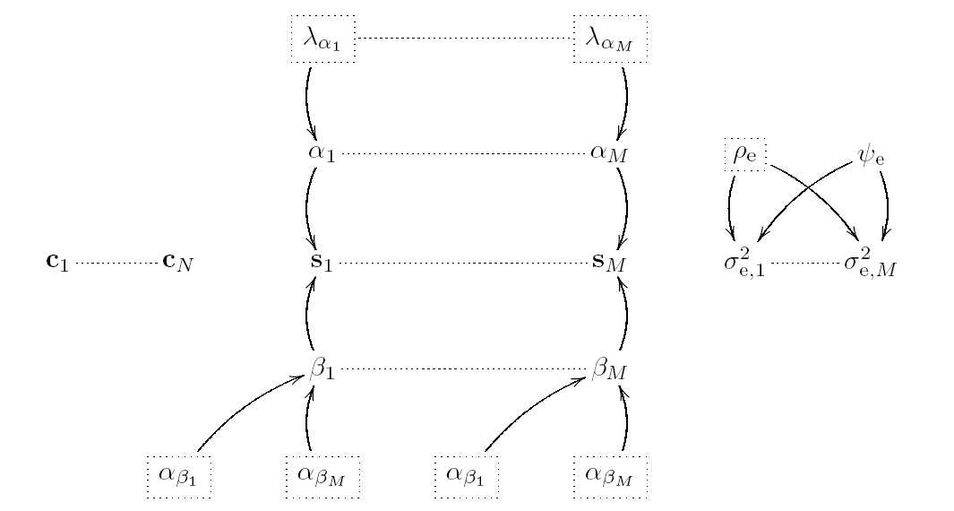
where $f\left(\mathbf{A}\right)$, $f\left(\mathbf{S}\big{|}{\boldsymbol{\sigma}}_{\mathrm{s}}^{2}\right)$ and $f\left({\boldsymbol{\sigma}}_{\mathrm{e}}^{2}\big{|}\rho_{\mathrm{e}},\psi_{\mathrm{e}}\right)$ have been defined previously. This hierarchical structure, depicted in the directed acyclic graph (DAG) of Fig. 1, allows one to integrate out the hyperparameters $\psi_{\mathrm{e}}$ and $\boldsymbol{\beta}$ from the joint distribution $f\left(\boldsymbol{\Theta},\boldsymbol{\Phi}|\mathbf{Y}\right)$, yielding:

$$\begin{split}f&\left(\mathbf{A},\mathbf{S},{\boldsymbol{\sigma}}_{\mathrm{e}}^{2},\boldsymbol{\alpha}\big{|}\mathbf{Y}\right)\propto\prod_{i=1}^{N}\left[\frac{\textbf{1}_{\mathbb{S}}({\mathbb{a}}_{i})}{\sigma_{\mathrm{e},i}^{L+2}}\exp\left(-\frac{\left\|{\mathbf{y}}_{i}-\mathbf{S}^{\mathsf{T}}{\mathbb{c}}_{i}\right\|^{2}}{2\sigma_{\mathrm{e},i}^{2}}\right)\right]\\ &\times\prod_{m=1}^{M}\left[\frac{\Gamma\left(L\alpha_{m}+\alpha_{\beta_{m}}+1\right)}{\left(\sum_{j=1}^{L}s_{m,j}+\beta_{\beta_{m}}\right)^{L\alpha_{j}+\alpha_{\beta_{m}}+1}}\right]\\ &\times\prod_{m=1}^{M}\left[\left(\prod_{j=1}^{L}\frac{s_{m,j}}{\Gamma\left(\alpha_{m}\right)}\right)^{\alpha_{m}-1}\textbf{1}_{\mathbb{R}^{L}_{+}}({\mathbf{s}}_{m})\right].\end{split}$$ (22)

The posterior distribution in (22) is clearly too complex to derive the classical Bayesian estimators of the unknown parameters, such as the minimum mean square error (MMSE) estimator or the maximum a posteriori (MAP) estimator. To overcome the difficulty, it is quite common to make use of MCMC methods to generate samples asymptotically distributed according to the exact posterior of interest [24]. The simulated samples are then used to approximate integrals by empirical averages for the MMSE estimator and to estimate the maximum of the posterior distribution for the MAP estimator. The next section proposes a Gibbs sampling strategy for the BSS of the spectral mixtures under the positivity and full additivity constraints.

Figure 1: DAG for the parameter priors and hyperpriors (the fixed parameters appear in dashed boxes).

IV Gibbs sampler

The Gibbs sampler is an iterative sampling strategy that consists of generating samples (denoted $\widetilde{\cdot}^{(t)}$) distributed according to the conditional distribution of each parameter. This section describes a Gibbs sampling strategy generating samples $\left(\widetilde{\mathbf{A}}^{(t)},\widetilde{\mathbf{S}}^{(t)},\left\{\widetilde{\boldsymbol{\sigma}}^{2}\right\}^{(t)},\widetilde{\boldsymbol{\alpha}}^{(t)}\right)$ asymptotically distributed according to (22). The main steps of the algorithm (denoted as Algorithm IV) are detailed from subsection IV-A to subsection IV-C.

Algorithm 1. Gibbs sampling algorithm for blind spectral source separation

• Initialization:

  1. sample the hyperparameter $\widetilde{\psi}_{\mathrm{e}}^{(0)}$ from the pdf in (18),

  2. for $i=1,\ldots,N$, sample the noise variance ${\left\{\widetilde{\sigma}_{\mathrm{e},i}^{2}\right\}^{(0)}}$ from the pdf in (14),

  3. for $m=1,\ldots,M$, sample the hyperparameter $\widetilde{\alpha}_{m}^{(0)}$ from the pdf in (16),

  4. for $m=1,\ldots,M$, sample the hyperparameter $\widetilde{\beta}_{m}^{(0)}$ from the pdf in (17),

  5. for $m=1,\ldots,M$, sample the source spectrum $\widetilde{{\mathbf{s}}}_{m}^{(t)}$ from the pdf in (12).

  6. Set $t\leftarrow 1$,

• Iterations: for $t=1,2,\ldots,$ do

  1. for $i=1,\ldots,N$, sample the concentration vector $\widetilde{{\mathbb{a}}}^{(t)}_{i}$ from the pdf in (25),

  2. sample the hyperparameter $\widetilde{\psi}_{\mathrm{e}}^{(t)}$ from the pdf in (26),

  3. for $i=1,\ldots,N$, sample the noise variance ${\left\{\widetilde{\sigma}_{\mathrm{e},i}^{2}\right\}^{(t)}}$ from the pdf in (27),

  4. for $m=1,\ldots,M$, sample the hyperparameter $\widetilde{\alpha}_{m}^{(t)}$ from the pdf in (28),

  5. for $m=1,\ldots,M$, sample the hyperparameter $\widetilde{\beta}_{m}^{(t)}$ from the pdf in (29),

  6. for $m=1,\ldots,M$, sample the source spectrum $\widetilde{{\mathbf{s}}}_{m}^{(t)}$ from the pdf in (30).

  7. Set $t\leftarrow t+1$.

IV-A Generation according to $f\left(\mathbf{A}|\mathbf{S},{\boldsymbol{\sigma}}_{\mathrm{e}}^{2},\mathbf{Y}\right)$

Straightforward computations yield for each observation:

$$f\left({\mathbb{a}}_{i}\left|\mathbf{S},\sigma_{\mathrm{e},i}^{2},{\mathbf{y}}_{i}\right.\right)\propto\exp\left[-\frac{\left({\mathbb{a}}_{i}-\boldsymbol{\mu}_{i}\right)^{\mathsf{T}}{\boldsymbol{\Lambda}}^{-1}_{i}\left({\mathbb{a}}_{i}-\boldsymbol{\mu}_{i}\right)}{2}\right]\textbf{1}_{\mathbb{T}}({\mathbb{a}}_{i}),$$ (23)

where:

$$\left\{\begin{split}{\boldsymbol{\Lambda}}_{i}&=\left[\frac{1}{\sigma_{\mathrm{e},i}^{2}}\left(\mathbf{S}_{\text{--}M,\boldsymbol{\cdot}}^{\mathsf{T}}-{\mathbf{s}}_{M}{\bf u}^{\mathsf{T}}\right)^{\mathsf{T}}\left(\mathbf{S}_{\text{--}M,\boldsymbol{\cdot}}^{\mathsf{T}}-{\mathbf{s}}_{M}{\bf u}^{\mathsf{T}}\right)\right]^{-1},\\ {\boldsymbol{\mu}}_{i}&={\boldsymbol{\Lambda}}_{i}\left[\frac{1}{\sigma_{\mathrm{e},i}^{2}}\left(\mathbf{S}_{\text{--}M,\boldsymbol{\cdot}}^{\mathsf{T}}-{\mathbf{s}}_{M}{\bf u}^{\mathsf{T}}\right)^{\mathsf{T}}\left({\mathbf{y}}_{i}-{\mathbf{s}}_{M}\right)\right],\end{split}\right.$$ (24)

with ${\bf u}=[1,\ldots,1]^{\mathsf{T}}\in\mathbb{R}^{M-1}$ and where $\mathbf{S}_{\text{--}M,\boldsymbol{\cdot}}$ denotes the matrix $\mathbf{S}$ from which the $M^{\mathrm{th}}$ row has been removed. As a consequence, ${\mathbb{a}}_{i}\big{|}\mathbf{S},\sigma_{\mathrm{e},i}^{2},{\mathbf{y}}_{i}$ is distributed according to a truncated Gaussian distribution on the simplex $\mathbb{S}$:

$${\mathbb{a}}_{i}\left|\mathbf{S},\sigma_{\mathrm{e},i}^{2},{\mathbf{y}}_{i}\right.\sim\mathcal{N}_{\mathbb{S}}\left(\boldsymbol{\mu}_{i},\boldsymbol{\Lambda}_{i}\right).$$ (25)

When the number $M$ of spectral sources is relatively small, the generation of ${\mathbb{a}}_{i}\left|\mathbf{S},\sigma_{\mathrm{e},i}^{2},{\mathbf{y}}_{i}\right.$ can be achieved using a standard Metropolis Hastings (MH) step. By choosing the Gaussian distribution $\mathcal{N}\left(\boldsymbol{\mu}_{i},\boldsymbol{\Lambda}_{i}\right)$ as proposal distribution for this MH step, the acceptance ratio of the MH algorithm reduces to $1$ if the candidate is inside the simplex $\mathbb{S}$ and $0$ otherwise. For higher dimension problems, the acceptance ratio of the MH algorithm can be small, leading to poor mixing properties. In such cases, an alternative strategy based on a Gibbs sampler can be used (see [25] and [26]).

IV-B Generation according to $f\left({\boldsymbol{\sigma}}_{\mathrm{e}}^{2}\left|\mathbf{A},\mathbf{S},\mathbf{Y}\right.\right)$

To sample according to $f\left({\boldsymbol{\sigma}}_{\mathrm{e}}^{2}\left|\mathbf{A},\mathbf{S},\mathbf{Y}\right.\right)$, it is very convenient to generate samples from $f\left({\boldsymbol{\sigma}}_{\mathrm{e}}^{2},\psi_{\mathrm{e}}\left|\mathbf{A},\mathbf{S},\mathbf{Y}\right.\right)$ by using the two following steps:

IV-B1 Generation according to $f\left(\psi_{\mathrm{e}}\left|{\boldsymbol{\sigma}}_{\mathrm{e}}^{2},\mathbf{A},\mathbf{S},\mathbf{Y}\right.\right)$

The conditional distribution is expressed as the following IG distribution:

$$\psi_{\mathrm{e}}\left|{\boldsymbol{\sigma}}_{\mathrm{e}}^{2},\rho_{\mathrm{e}}\right.\sim\mathcal{IG}\left(\frac{N\rho_{\mathrm{e}}}{2},\frac{1}{2}\sum_{i=1}^{N}\frac{1}{\sigma_{\mathrm{e},i}^{2}}\right).$$ (26)

IV-B2 Generation according to $f\left({\boldsymbol{\sigma}}_{\mathrm{e}}^{2}\left|\psi_{\mathrm{e}},\mathbf{A},\mathbf{S},\mathbf{Y}\right.\right)$

After a careful examination of $f\left({\boldsymbol{\sigma}}_{\mathrm{e}}^{2},\mathbf{A},\psi_{\mathrm{e}}\big{|}\mathbf{S},\mathbf{Y}\right)$, it can be deduced that the conditional distribution of the noise variance in each observation spectrum is the following IG distribution:

$$\sigma_{\mathrm{e},i}^{2}\left|\psi_{\mathrm{e}},{\mathbb{a}}_{i},\mathbf{S},{\mathbf{y}}_{i}\right.\sim\mathcal{IG}\left(\frac{\rho_{\mathrm{e}}+L}{2},\frac{\psi_{\mathrm{e}}+\left\|{\mathbf{y}}_{i}-\mathbf{S}{\mathbb{c}}_{i}^{\mathsf{T}}\right\|^{2}}{2}\right).$$ (27)

IV-C Generation according to $f\left(\mathbf{S}\left|\mathbf{A},{\boldsymbol{\sigma}}_{\mathrm{e}}^{2},\mathbf{Y}\right.\right)$

This generation can be achieved thanks to the three following steps, as in [8].

IV-C1 Generation according to $f\left(\boldsymbol{\alpha}\left|\boldsymbol{\beta},\mathbf{S},\mathbf{A},{\boldsymbol{\sigma}}_{\mathrm{e}}^{2},\mathbf{Y}\right.\right)$

From the joint distribution $f\left(\mathbf{A},\mathbf{S},{\boldsymbol{\sigma}}_{\mathrm{e}}^{2},\boldsymbol{\alpha},\boldsymbol{\beta}|\mathbf{Y}\right)$, we can express the posterior distribution of $\alpha_{m}$ ($m=1,\ldots,M$) as:

$$f\left(\alpha_{m}\big{|}{\mathbf{s}}_{m},\beta_{m}\right)\propto\prod_{j=1}^{L}\left[\frac{\beta_{m}^{\alpha_{m}}}{\Gamma\left(\alpha_{m}\right)}s_{m,j}^{\alpha_{m}}\right]e^{-\lambda_{\alpha_{m}}\alpha_{m}}\textbf{1}_{\mathbb{R}^{+}}(\alpha_{m}).$$ (28)

This posterior is not easy to simulate as it does not belong to a known distribution family. Therefore, an MH step is required to generate samples $\widetilde{\alpha}_{m}^{(t)}$ distributed according to (28). The reader is invited to consult [8] for more details regarding the choice of the instrumental distribution in order to obtain a high acceptance rate for the MH algorithm.

IV-C2 Generation according to $f\left(\boldsymbol{\beta}\left|\boldsymbol{\alpha},\mathbf{S},\mathbf{A},{\boldsymbol{\sigma}}_{\mathrm{e}}^{2},\mathbf{Y}\right.\right)$

Similarly, the posterior distribution of the hyperparameter vector $\boldsymbol{\beta}$ can be determined by looking at the joint distribution $f\left(\mathbf{A},\mathbf{S},{\boldsymbol{\sigma}}_{\mathrm{e}}^{2},\boldsymbol{\alpha},\boldsymbol{\beta}|\mathbf{Y}\right)$. In this case, the posterior distribution of the individual hyperparameter $\beta_{m}$ ($m=1,\ldots,M$) is the following Gamma distribution:

$$\beta_{m}\big{|}\alpha_{m},{\mathbf{s}}_{m}\sim\mathcal{G}\left(1+L\alpha_{m}+\alpha_{\alpha_{m}},\sum_{j=1}^{L}s_{m,j}+\beta_{\alpha_{m}}\right).$$ (29)

IV-C3 Generation according to $f\left(\mathbf{S}\left|\boldsymbol{\alpha},\boldsymbol{\beta},\mathbf{A},{\boldsymbol{\sigma}}_{\mathrm{e}}^{2},\mathbf{Y}\right.\right)$

Finally, the posterior distribution of the source observed in the $j^{\text{th}}$ spectral band is:

$$f\left(s_{m,j}\big{|}\alpha_{m},\beta_{m},\mathbf{A},{\boldsymbol{\sigma}}_{\mathrm{e}}^{2},\mathbf{Y}\right)\propto s_{m,j}^{\alpha_{m}-1}\textbf{1}_{\mathbb{R}^{+}}(s_{m,j})\exp\left[-\frac{\left(s_{m,j}-\mu_{m,j}\right)^{2}}{2\delta^{2}_{m}}-\beta_{m}s_{m,j}\right],$$ (30)

with

$$\left\{\begin{array}[]{l}\delta^{2}_{m}=\left[\sum_{i=1}^{N}\frac{c_{i,m}^{2}}{\sigma_{\mathrm{e},i}^{2}}\right]^{-1},\\ \mu_{m,j}=\frac{1}{\delta^{2}_{m}}\sum_{i=1}^{N}\frac{c_{i,m}\epsilon_{i,j}^{(-m)}}{\sigma_{\mathrm{e},i}^{2}},\end{array}\right.$$ (31)

where $\epsilon_{i,j}^{(-m)}=y_{i,j}-\sum_{k\neq m}c_{i,k}s_{k,j}$. The generation of samples distributed according to (30) is achieved by using an MH algorithm whose proposal is a positive truncated normal distribution [8]. The generation according to the positive truncated Gaussian distribution can be achieved thanks to an accept-reject scheme with multiple proposal distributions (see [27, 25, 28] for details).

V Experimental results with synthetic data

This section presents some experiments performed on synthetic data to illustrate the performance of the proposed Bayesian spectral unmixing algorithm.

V-A Mixture synthesis

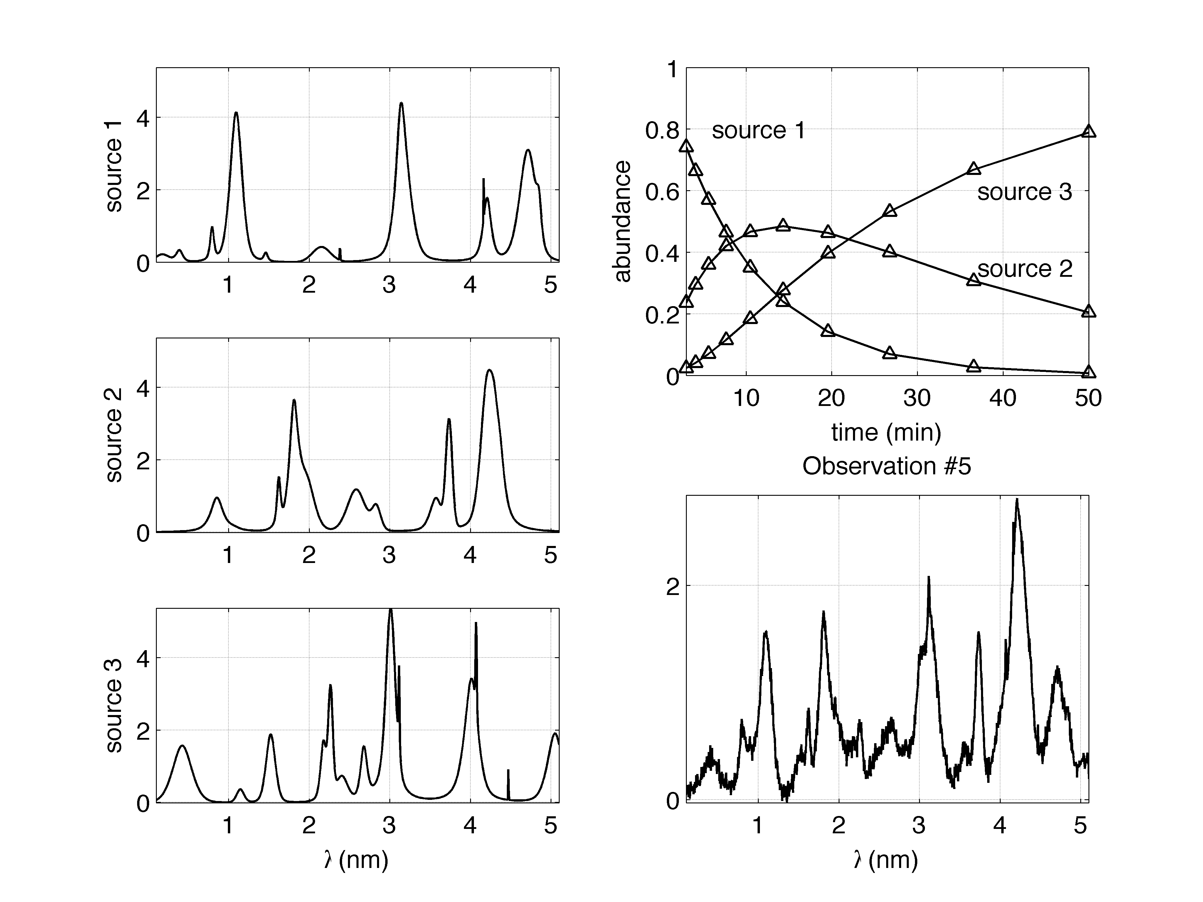
The spectral sources have been simulated to get signals similar to absorption spectroscopy data. Each spectrum is obtained as a superposition of Gaussian and Lorentzian functionals with randomly chosen parameters (location, amplitude and width) [8]. Figure 2 (left) shows an example of $M=3$ source signals of $L=1000$ spectral bands. For this application, a “spectral” band corresponds to a given value of the wavelength $\lambda$ (expressed in nanometers). The mixing coefficients have been chosen to obtain evolution profiles similar to component abundance variation in a kinetic reaction, as depicted in Figure 2 (top, right). The abundance fraction profiles have been simulated for $N=10$ observation times, which provides $N=10$ observation spectra. An i.i.d. Gaussian sequence has been added to each observation with appropriate standard deviation to have a signal to noise ratio (SNR) equal to $20$dB. One typical realization of the observed spectra is shown in Figure 2 (bottom, right).

Figure 2: Left: example of $M=3$ simulated spectral sources where the $x$-axis corresponds to the wavelength expressed in $nm$ and the $y$-axis corresponds to the absorbance of the spectra. Right, top: abundance evolution profiles. Right, bottom: one typical realization of the observed spectra.

V-B Separation with non-negativity and full additivity constraints

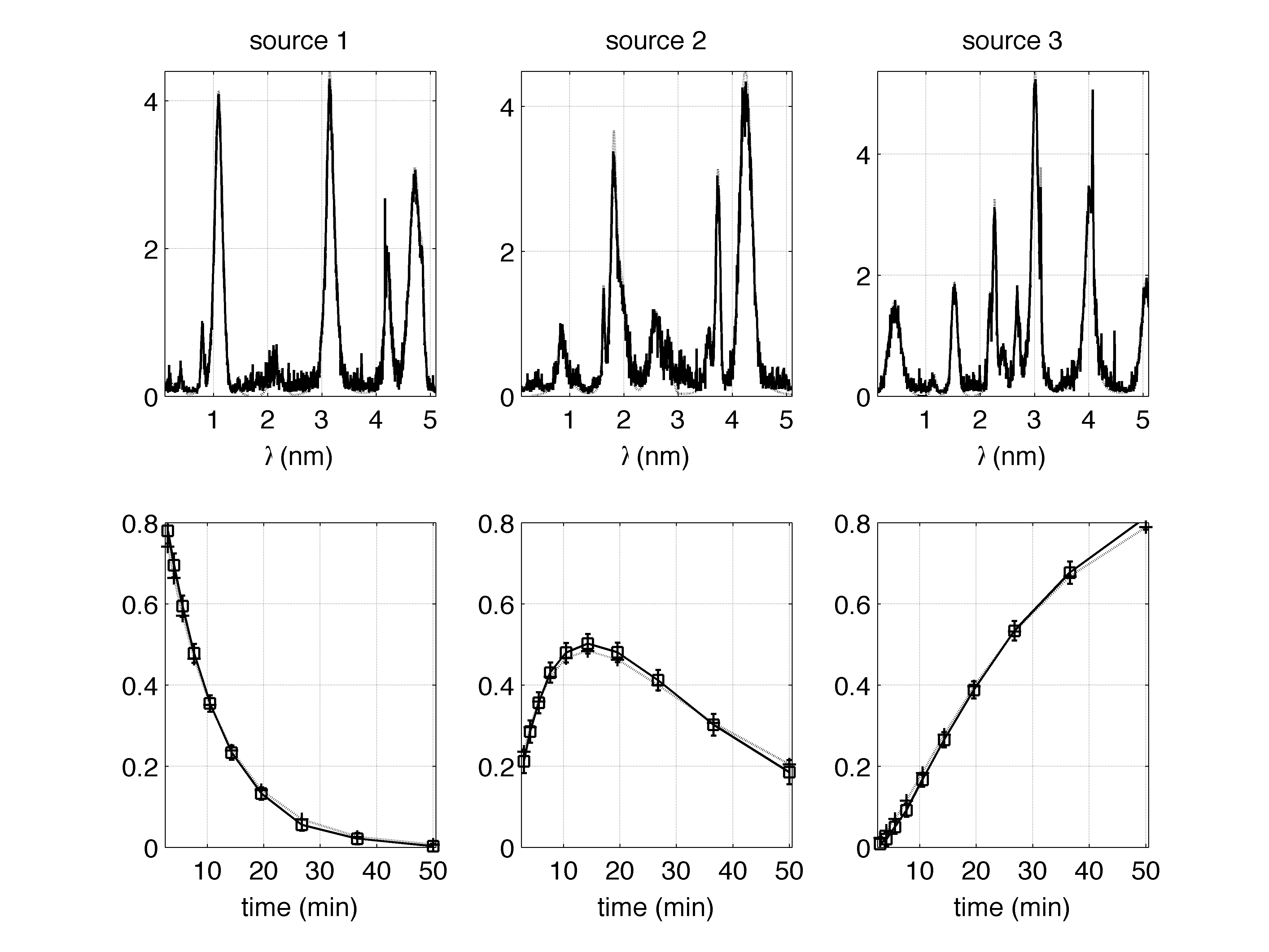
Figure 3 summarizes the result of a Monte Carlo simulation with $100$ runs where the mixing matrix has been kept unchanged, while new sources and noise sequences have been generated at each run. Figure 3-a shows a comparison between the true concentrations (cross) and their MMSE estimates (circles) obtained for a Markov chain of $N_{\textrm{MC}}=1000$ iterations including $N_{\textrm{b-i}}=200$ burn-in iterations. These estimates have been computed according to the MMSE principle ($i=1,\ldots,M$):

$$\hat{{\mathbb{a}}}_{i}=\frac{1}{N_{r}}\sum_{t=1}^{N_{r}}\widetilde{{\mathbb{a}}}^{(N_{\textrm{b-i}}+t)}_{i},$$ (32)

where $N_{r}=N_{\textrm{MC}}-N_{\textrm{b-i}}$ is the number of iterations used for the estimation. The estimated abundances are clearly in good agreement with the actual abundances and the estimates satisfy the positivity and full additivity constraints. By comparing figures 2 (left) and 3 (top), it can be observed that the source signals have also been correctly estimated.

Figure 3: Top: Simulated (dotted) and estimated (continuous line) source spectra. Bottom: Simulated values (cross) and MMSE estimates (circles) of the abundances. Error bars indicate the estimated 95% confidence intervals from the simulated Markov chain.

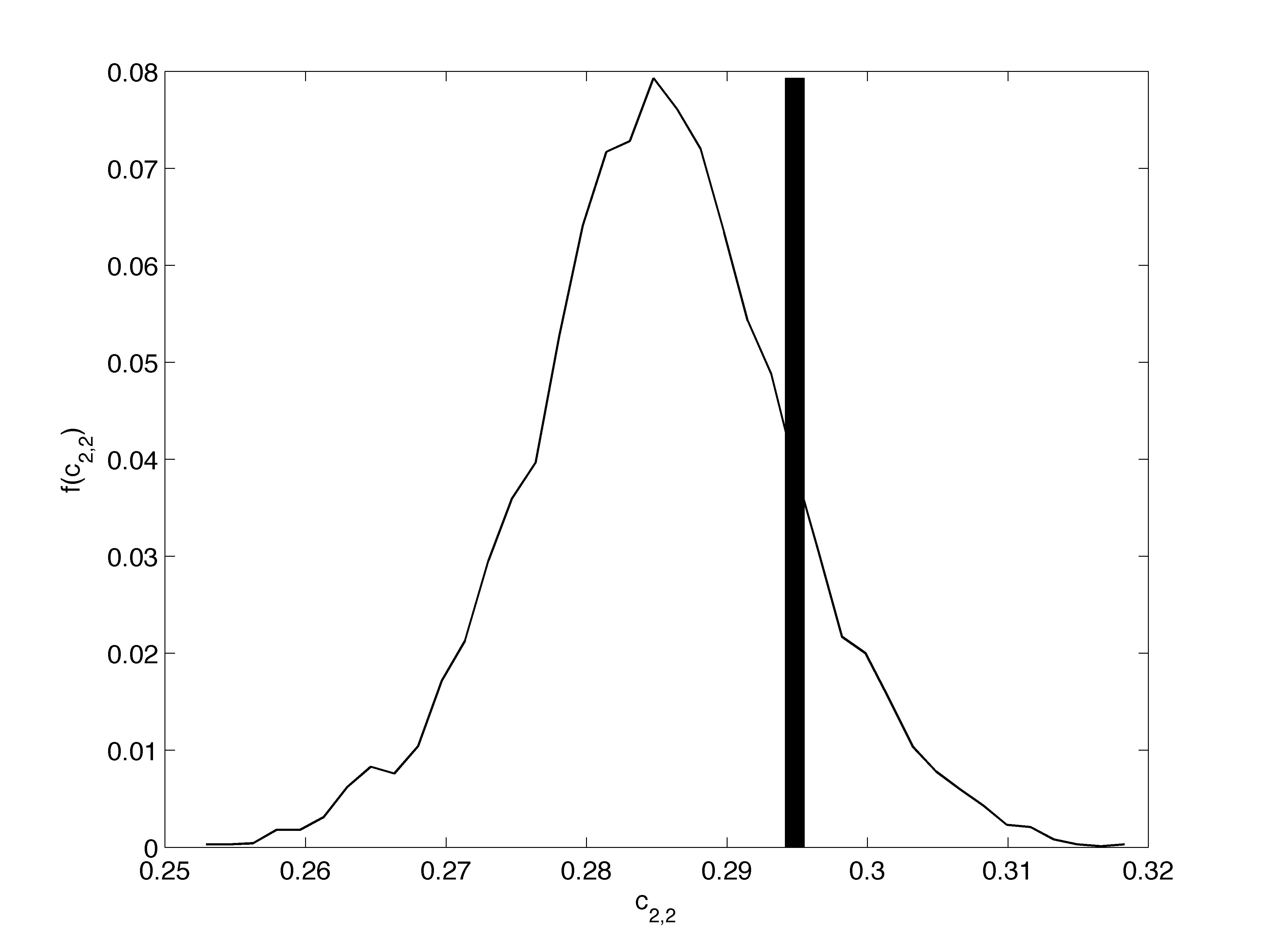
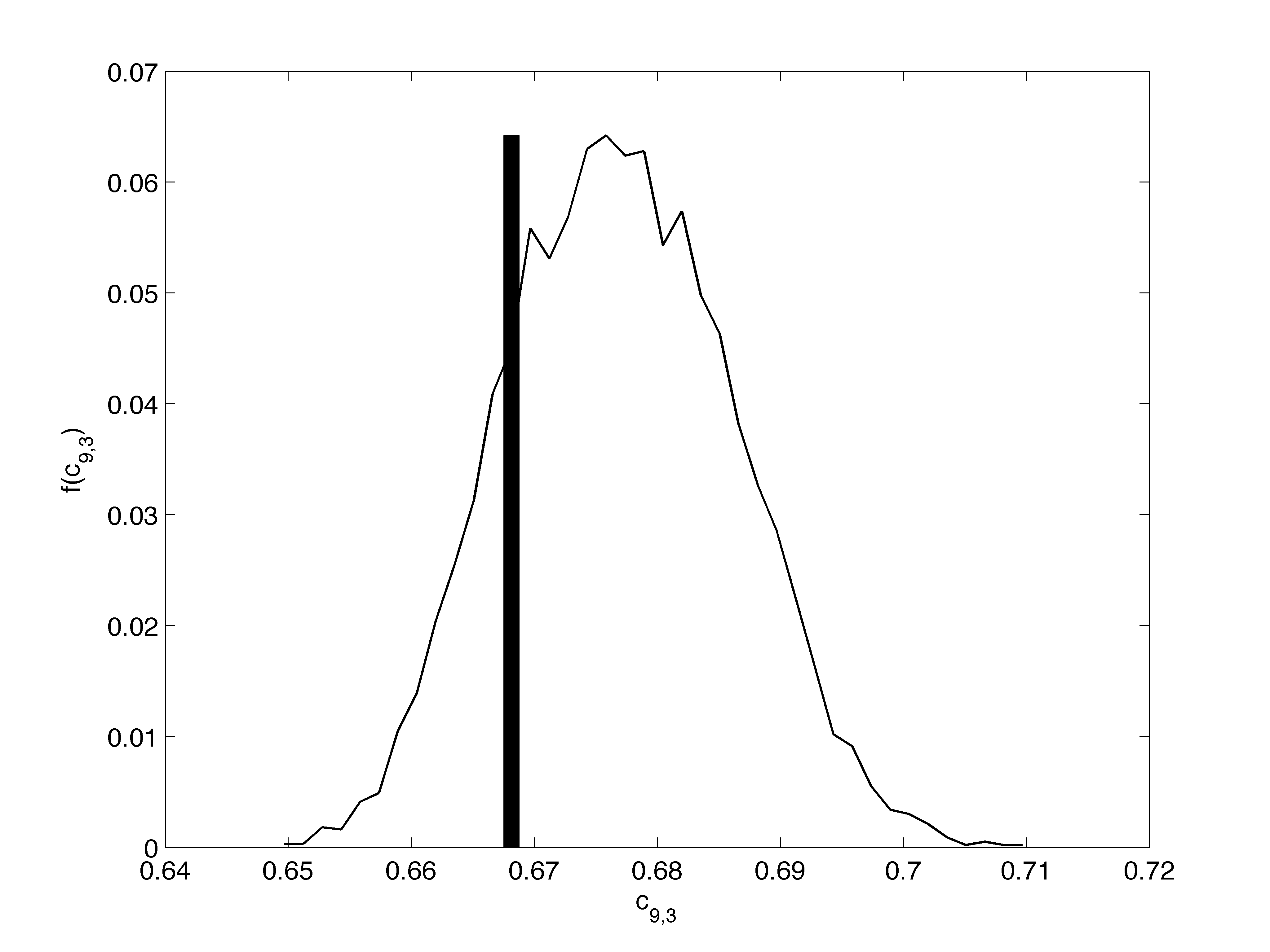
It is interesting to note that the proposed algorithm generates samples distributed according to the posterior distribution of the unknown parameters $f\left(\mathbf{A},\mathbf{S},{\boldsymbol{\sigma}}_{\mathrm{e}}^{2},{\boldsymbol{\alpha}}\big{|}\mathbf{Y}\right)$. These samples can be used to obtain the posterior distributions of the concentrations or the source spectra. As an example, typical posterior distributions for two mixing coefficients are depicted in figure 4. These posteriors are in good agreement with the theoretical posterior distributions in (25), i.e. truncated Gaussian distributions.

Figure 4: Left (resp. right): posterior distribution of the concentration of the $2^{\text{nd}}$ (resp. $3^{\text{rd}}$) spectral component in the mixture observed at index time $i=2$ (resp. $i=9$). The actual values appear as black bars.

V-C Monitoring sampler convergence

An important issue when using MCMC methods is convergence monitoring. The Gibbs sampler detailed in section IV generates random samples $\left(\widetilde{\mathbf{A}}^{(t)},\widetilde{\mathbf{S}}^{(t)},\widetilde{\boldsymbol{\sigma}}^{2(t)},\widetilde{\boldsymbol{\alpha}}^{(t)}\right)$ asymptotically distributed according to the posterior distribution in (22). The quantities of interest, i.e. the concentration coefficients and the source spectra, are then approximated by empirical averages according to (32). However, two essential parameters have to be tuned: the length $N_{\mathrm{MC}}$ of the constructed Markov chain and the length $N_{\mathrm{b-i}}$ of the burn-in period, i.e. the number of simulated samples to be discarded before computing the averages. This section reports some works conducted to ensure the convergence of the proposed algorithm and the accuracy of the estimation for the unknown parameters.

First, the burn-in period $N_{\textrm{b-i}}=200$ has been determined thanks to the popular potential scale reduction factor (PSRF). The PSRF was introduced by Gelman and Rubin [29] and has been widely used in the signal processing literature (see for instance [30, 31, 32]). It consists of running several parallel Markov chains and computing the following criterion:

$$\hat{\rho}=\left(1-\frac{1}{N_{r}}\right)\left[1+\frac{1}{(N_{r}-1)}\frac{B(\kappa)}{W(\kappa)}\right],$$ (33)

where $W$ and $B$ are the within and between-sequence variances of the parameter $\kappa$, respectively. Different choices for $\kappa$ can be used for our source separation problem. Here, we consider the parameters $\sigma_{\mathrm{e},i}^{2}$ ($i=1,\ldots,N$) as recommended in [33]. Table I shows the PSRF obtained for the $N=10$ observation times computed from $M=10$ Markov chains. All these values of $\sqrt{\hat{\rho}}$ confirm the good convergence of the sampler since a recommendation for convergence assessment is $\sqrt{\hat{\rho}}<1.2$ [34, p. 332].

TABLE I: Potential scale reduction factors of $\sigma_{\mathrm{e},i}^{2}$ computed from $M=10$ Markov chains.

Obs. index	$\sqrt{\hat{\rho}}$	Obs. index	$\sqrt{\hat{\rho}}$
1	1.0048	2	1.0013
3	1.0027	4	0.9995
5	1.0097	6	1.0078
7	1.0001	8	0.9994
9	1.0080	10	1.0288

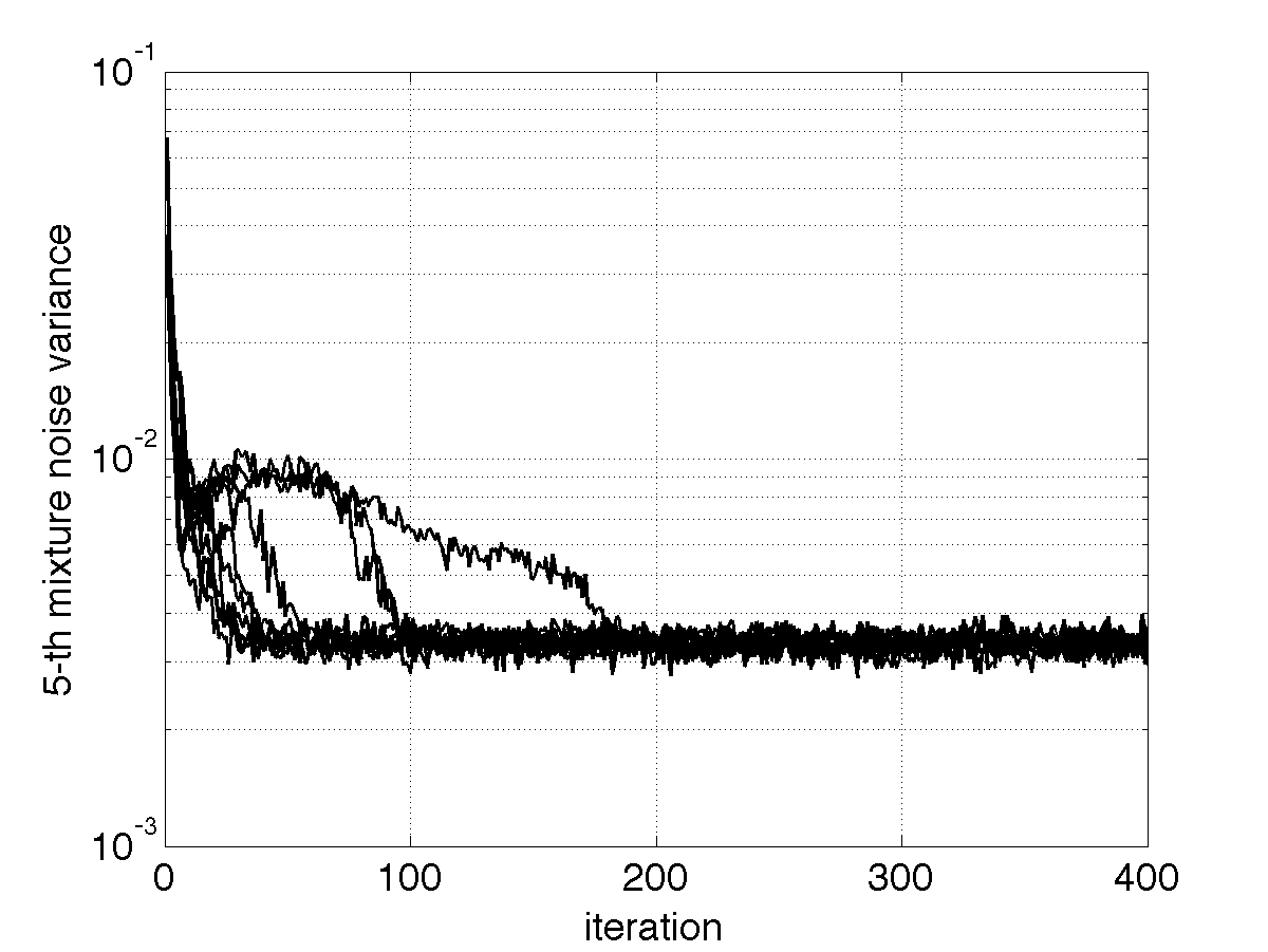
The Markov chain convergence can also be monitored by a graphical supervision of the generated samples of the noise variances. As an illustration, the outputs of $10$ Markov chains for one of the parameter $\sigma_{\mathrm{e},i}^{2}$ are depicted in figure 5. All the generated samples converge to a similar value after a short burn-in period ($200$ iterations, in this example).

Figure 5: Outputs of $M=10$ Markov chains for the parameter $\sigma_{\mathrm{e},5}^{2}$.

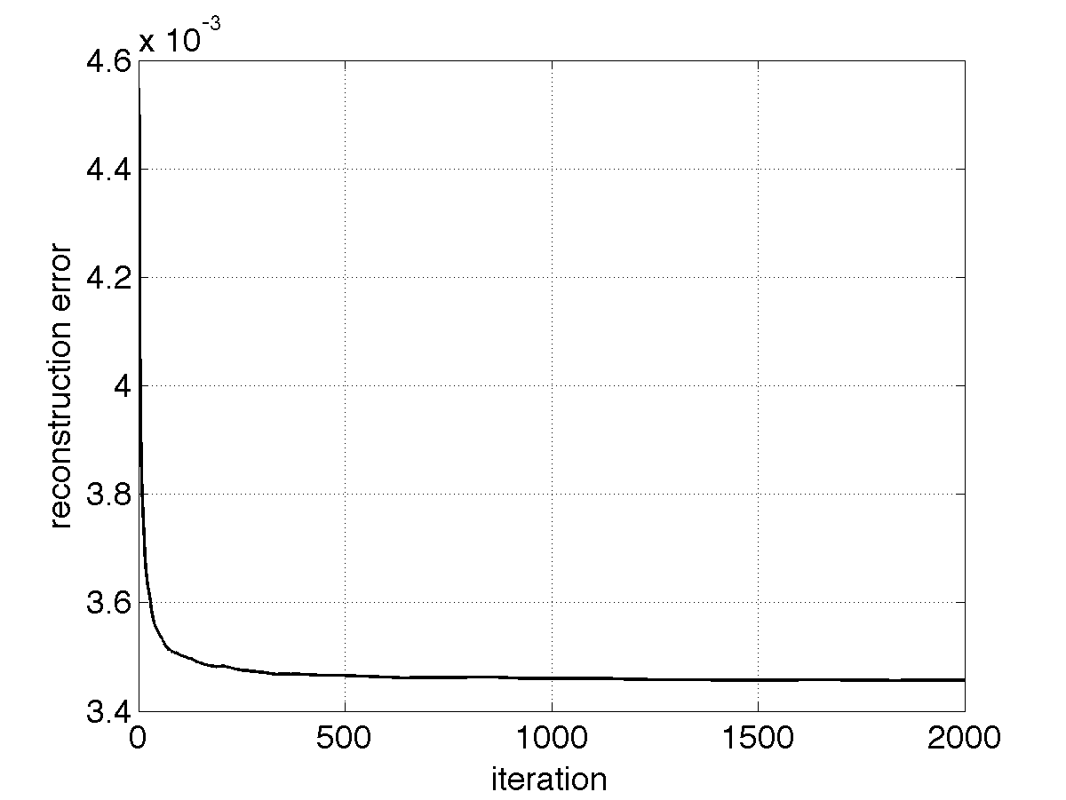
Once the number of burn-in iterations has been fixed, the number of iterations necessary to obtain accurate estimates of the unknown parameters via (32) has to be adjusted. This paper proposes to evaluate $N_{r}$ with appropriate graphical evaluations (see [35, p. 28] for motivations). Figure 6 shows the reconstruction error associated to the different spectra defined as:

$$e_{r}^{2}(p)=\dfrac{1}{NL}\sum_{i=1}^{N}\left\|{\mathbf{y}}_{i}-\left(\hat{{\mathbb{c}}_{i}}^{(p)}\hat{\mathbf{S}}^{(p)}\right)^{\mathsf{T}}\right\|^{2},$$ (34)

where $\hat{{\mathbb{c}}_{i}}^{(p)}$ and $\hat{\mathbf{S}}^{(p)}$ are the MMSE estimates of the abundance vector ${\mathbb{c}}_{i}$ and the source matrix $\mathbf{S}$ computed after $N_{\textrm{b-i}}=200$ burn-in iterations and $N_{r}=p$ iterations. The number of iterations $N_{r}$ required to compute the empirical averages following the MMSE estimator (32) can be fixed to ensure the reconstruction error is below a predefined threshold. Figure 6 shows that a number of iterations $N_{r}=500$ is sufficient to ensure a good estimation of the quantities of interest $\mathbf{C}$ and $\mathbf{S}$.

Figure 6: Evolution of the reconstruction error with respect to the iteration number (with a burn-in of $N_{\textrm{b-i}}=200$ iterations).

V-D Comparison with other BSS algorithms

The proposed Bayesian approach has been compared with other standard BSS methods. Synthetic mixtures have been processed by the non-negative ICA (NN-ICA) algorithm proposed by Plumbley and Oja [36], the iterative NMF method described in [7] and the Bayesian Positive Source Separation (BPSS) algorithm introduced in [8].

All these methods do not include the full additivity constraint. To evaluate the relevance of this additional constraint, ad hoc re-scaled versions of these methods have also been considered. Simulations have been conducted by applying the $4$ algorithms using $100$ Monte Carlo runs, each run being associated to a randomly generated source. Table II shows the normalized mean square errors (NMSEs) for the estimated sources and abundance matrices as defined in [37]:

$$\begin{split}\mathrm{NMSE}\left(\mathbf{S}\right)&=\sum_{m=1}^{M}\frac{\left\|{\mathbf{s}}_{m}-\hat{\mathbf{s}}_{m}\right\|^{2}}{\left\|{\mathbf{s}}_{m}\right\|^{2}},\\ \mathrm{NMSE}\left(\mathbf{C}\right)&=\sum_{i=1}^{N}\frac{\left\|{\mathbb{c}}_{i}-\hat{\mathbf{c}}_{i}\right\|^{2}}{\left\|{\mathbb{c}}_{i}\right\|^{2}}.\end{split}$$ (35)

In addition, the estimation performances have been compared in terms of dissimilarity. Denoted $\mathrm{diss}\left(\cdot,\cdot\right)$, it measures how the estimated source spectrum differs from the reference one [38] and is defined by:

$$\mathrm{diss}\left({\mathbf{s}}_{m},\hat{\mathbf{s}}_{m}\right)=\sqrt{1-\mathrm{corr}\left({\mathbf{s}}_{m},\hat{\mathbf{s}}_{m}\right)^{2}},$$ (36)

where $\mathrm{corr}(\mathbf{s}_{m},\hat{\mathbf{s}}_{m})$ is the correlation coefficient between $\mathbf{s}_{m}$ and its estimate $\hat{\mathbf{s}}_{m}$. Consequently the average dissimilarity over the $M$ sources is reported in Table II.

TABLE II: Estimation performance for different BSS algorithms ($100$ Monte Carlo runs).

	$\mathrm{NMSE}\left(\mathbf{S}\right)$	$\mathrm{NMSE}\left(\mathbf{C}\right)$	Av. $\mathrm{Diss}\left(\mathbf{S}\right)$	Time (min)
Proposed approach	0.0071	0.0024	13.9 %	44
BPSS	0.0121	0.0025	13.4 %	45
re-scaled BPSS	0.0126	0.0023	13.4 %	45
NN-ICA	0.0613	0.0345	20.0 %	3
re-scaled NN-ICA	0.0602	0.0384	19.4 %	3
NMF	0.2109	1.9149	22.6 %	1
re-scaled NMF	0.0575	0.0496	24.5 %	1

These results demonstrate that an ad hoc re-scaling of the results obtained by NMF techniques is not always an efficient means to improve the estimation performance. Indeed, the ad hoc re-scaled version of NMF provides lower MSEs than the corresponding standard algorithms. On the other hand, this constraint does not significantly improve the NN-ICA or the BPSS algorithms. As far as the Bayesian algorithms are concerned, they clearly provide better estimation performance than the non-Bayesian approaches. However, the proposed fully constrained algorithm clearly outperforms the two BPSS algorithms, especially regarding the source estimation.

The computation times required by each of these algorithms are also reported in Table II for a MATLAB implementation on a $2.2$GHz Intel Core 2. This shows that the complexities of the proposed method and BPSS algorithms are quite similar and higher than the complexities of the NN-ICA and MNF algorithms. This seems to be the price to pay to obtain significantly better estimation performances.

V-E Modified Bayesian models with other source priors

As it has been mentioned previously, several distributions can be chosen as priors for the source spectra, provided these distributions have positive supports. The previous HBM studied in section III-B2 is based on Gamma distributions as source priors. However, simpler models can be obtained for instance by choosing exponential priors with different scale parameters $\sigma_{\mathrm{s},m}^{2}$:

$$f\left({\mathbf{s}}_{m}\big{|}\sigma_{\mathrm{s},m}^{2}\right)\propto\prod_{j=1}^{L}\frac{1}{\sigma_{\mathrm{s},m}^{2}}\exp\left(-\frac{s_{m,j}}{2\sigma_{\mathrm{s},m}^{2}}\right)\textbf{1}_{\mathbb{R}^{+}}(s_{m,j}),$$ (37)

or positive truncated Gaussian distribution with different hidden variances $\sigma_{\mathrm{s},m}^{2}$:

$$f\left({\mathbf{s}}_{m}\big{|}\sigma_{\mathrm{s},m}^{2}\right)\propto\prod_{j=1}^{L}\frac{1}{\sigma_{\mathrm{s},m}^{2}}\exp\left(-\frac{s_{m,j}^{2}}{2\sigma_{\mathrm{s},m}^{2}}\right)\textbf{1}_{\mathbb{R}^{+}}(s_{m,j}).$$ (38)

The resulting Bayesian algorithms are simpler since only one hyperparameter $\sigma_{\mathrm{s},m}^{2}$ has to be adjusted for each source.

For both choices, conjugate IG distributions $\mathcal{IG}\left(\frac{\rho_{\mathrm{s}}}{2},\frac{\psi_{\mathrm{s}}}{2}\right)$ are chosen as prior distributions for the hyperparameters $\sigma_{\mathrm{s},m}^{2}$, $m=1,\ldots,M$. After integrating out the hyperparameter vector $\boldsymbol{\Phi}=\left\{\psi_{\mathrm{e}},{\boldsymbol{\sigma}}_{\mathrm{s}}^{2}\right\}$, the posterior distribution in (22) can be expressed as:

$$f\left(\mathbf{A},\mathbf{S},{\boldsymbol{\sigma}}_{\mathrm{e}}^{2}\big{|}\mathbf{Y}\right)\propto\prod_{m=1}^{M}T\left({\mathbf{s}}_{m},\rho_{\mathrm{s}},\psi_{\mathrm{s}}\right)\textbf{1}_{\mathbb{R}^{L}_{+}}({\mathbf{s}}_{m})\prod_{i=1}^{N}\left[\frac{1}{\sigma_{e,i}^{L+2}}\exp\left(-\frac{\left\|{\mathbf{y}}_{i}-\mathbf{S}^{\mathsf{T}}{\mathbb{c}}_{i}\right\|^{2}}{2\sigma_{\mathrm{e},i}^{2}}\right)\textbf{1}_{\mathbb{S}}({\mathbb{a}}_{i})\right].$$ (39)

The scalar $T\left({\mathbf{s}}_{m},\rho_{\mathrm{s}},\psi_{\mathrm{s}}\right)$ depends on the prior distribution used for the source spectra:

$$T\left({\mathbf{s}}_{m},\rho_{\mathrm{s}},\psi_{\mathrm{s}}\right)=\left\{\begin{array}[]{ll}\left[\psi_{\mathrm{s}}+\left\|{\mathbf{s}}_{m}\right\|_{1}\right]^{-\frac{L+\rho_{\mathrm{s}}}{2}},&\hbox{ for exponential priors,}\\ \left[\psi_{\mathrm{s}}+\left\|{\mathbf{s}}_{m}\right\|_{2}^{2}\right]^{-\frac{L+\rho_{\mathrm{s}}}{2}},&\hbox{ for truncated Gaussian priors.}\\ \end{array}\right.$$ (40)

In the Gibbs sampling strategy presented in section IV, the generation according to $f\left(\mathbf{S}\left|\mathbf{A},{\boldsymbol{\sigma}}_{\mathrm{e}}^{2},\mathbf{Y}\right.\right)$ in subsection IV-C is finally achieved using the following two steps:

• generation according to $f\left({\boldsymbol{\sigma}}_{\mathrm{s}}^{2}\left|\mathbf{S},\mathbf{A},{\boldsymbol{\sigma}}_{\mathrm{e}}^{2},\mathbf{Y}\right.\right)$:

  $$\sigma_{\mathrm{s},m}^{2}\big{|}{\mathbf{s}}_{m}\sim\mathcal{IG}\left(L+\rho_{\mathrm{s}},\psi_{\mathrm{s}}+\left\|{\mathbf{s}}_{m}\right\|^{b}_{\ell_{b}}\right),$$ (41)

  where $b=1$ for the exponential prior and $b=2$ otherwise,

• generation according to $f\left(\mathbf{S}\left|{\boldsymbol{\sigma}}_{\mathrm{s}}^{2},\mathbf{A},{\boldsymbol{\sigma}}_{\mathrm{e}}^{2},\mathbf{Y}\right.\right)$

  $${\mathbf{s}}_{m}\left|{\boldsymbol{\sigma}}_{\mathrm{s}}^{2},\mathbf{A},{\boldsymbol{\sigma}}_{\mathrm{e}}^{2},\mathbf{Y}\right.\sim\mathcal{N}^{+}\left(\boldsymbol{\lambda}_{m},\delta_{m}^{2}\textbf{I}_{L}\right),$$ (42)

  where $\boldsymbol{\lambda}_{m}$ and $\delta_{m}^{2}$, similar to (31), are derived following the model in [8].

Table III reports the NMSEs (computed from $100$ Monte Carlo runs following (35)) for the sources and concentration matrices estimated by the different Bayesian algorithms. The results are significantly better when employing the Gamma distribution, which clearly indicates that the Gamma prior seems to be the best choice to model the distribution of the sources when analyzing spectroscopy data.

TABLE III: NMSE for different source priors ($100$ Monte Carlo runs).

	Gamma	Truncated Gaussian	Exponential
$\mathrm{NMSE}\left(\mathbf{S}\right)$	0.0071	0.0269	0.0110
$\mathrm{NMSE}\left(\mathbf{C}\right)$	0.0024	0.0089	0.0029

VI Separation of chemical mixtures monitored by Raman spectroscopy

Calcium carbonate is a chemical material used commercially for a large variety of applications such as filler for plastics or paper. Depending on operating conditions, calcium carbonate crystallizes as calcite, aragonite or vaterite. Calcite is the most thermodynamically stable of the three, followed by aragonite or vaterite. Globally, the formation of calcium carbonate by mixing two solutions containing respectively calcium and carbonate ions takes place in two well distinguished steps. The first step is the precipitation one. This step is very fast and provides a mixture of calcium carbonate polymorphs. The second step (a slow process) represents the phase transformation from the unstable polymorphs to the stable one (calcite). The physical properties of the crystallized product depend largely on the polymorphic composition, so it is necessary to quantify these polymorphs when they are mixed. Several techniques based on infrared spectroscopy (IR), X ray-diffraction (XRD) or Raman spectroscopy (RS) can be used to determine the composition of CaCO₃ polymorph mixtures. However, contrary to XRD and IR, RS is a faster method since it does not require a sample preparation and is a promising tool for an online polymorphic composition monitoring. In our case, the crystallization process of calcium carbonate is carried out in $5\textrm{mol$/$L}$ NaCl solutions, which correspond to a real industrial situation. Under the industrial conditions, the calcite is the desired product.

The main purpose of this experiment is to show how the proposed constrained BSS method can be used for processing Raman spectroscopy data to study the relation between polymorphs and temperature and to explore favorable conditions for calcite formation in saline solutions.

VI-A Mixture preparation and data acquisition

Calcium chloride and sodium carbonate separately dissolved in sodium chloride solutions of the same concentration ($5\textrm{mol$/$L}$) were rapidly mixed to precipitate calcium carbonate. A $100$mL solution containing $0.625$M of Na₂CO₃ and $5$M of NaCl was added to a $2.5$L solution containing $0.025$M of CaCl₂ and $5$M of NaCl (the precipitation is carried out under stoichiometric conditions). A preliminary investigation detailed in [39] suggested that the temperature and the aging time are the most important factors that can affect the polymorphic composition. Therefore the experiments were operated in a temperature range between $20$ C and $70$ C and retaining several aging times of the precipitated mixture. A sample was collected $2$ minutes after the beginning of the experiment to determine the polymorphic composition at the end of the precipitation step. Then, samples were collected at regular time intervals to follow the polymorph transformation.

Raman Spectra were collected on a Jobin-Yvon T$64000$ spectrometer equipped with an optical microscope, a threefold monochromator, and a nitrogen-cooled CCD camera. The excitation was induced by a laser beam of argon Spectra Physic Laser Stability $2017$ at a wavelength of $514.5$nm. The beam was focused using a long-frontal x$50$ objective (numerical aperture $0.5$) on an area of about $3\mu$m². The laser power on the sample was approximately $20$mW and the acquisition time was 1 minute. The spectral resolution was $3$cm^-1, with a wavenumber precision better than $1$cm^-1. The Raman spectra were collected at five points, which were randomly distributed throughout the mixture. The average of all spectra was considered as the Raman spectrum of the corresponding mixture for the considered temperature value and aging time. Raman spectra were collected $2$ minutes after the beginning of the experiment for various temperatures ranging between $20$ C and $70$ C in order to determine the influence of temperature on the polymorph precipitation. Moreover for each temperature, Raman spectra were collected at regular time intervals for monitoring phase transformation. Finally, a total of $N=37$ Raman spectra of $L=477$ wavelengths have been obtained.

VI-B Data preprocessing

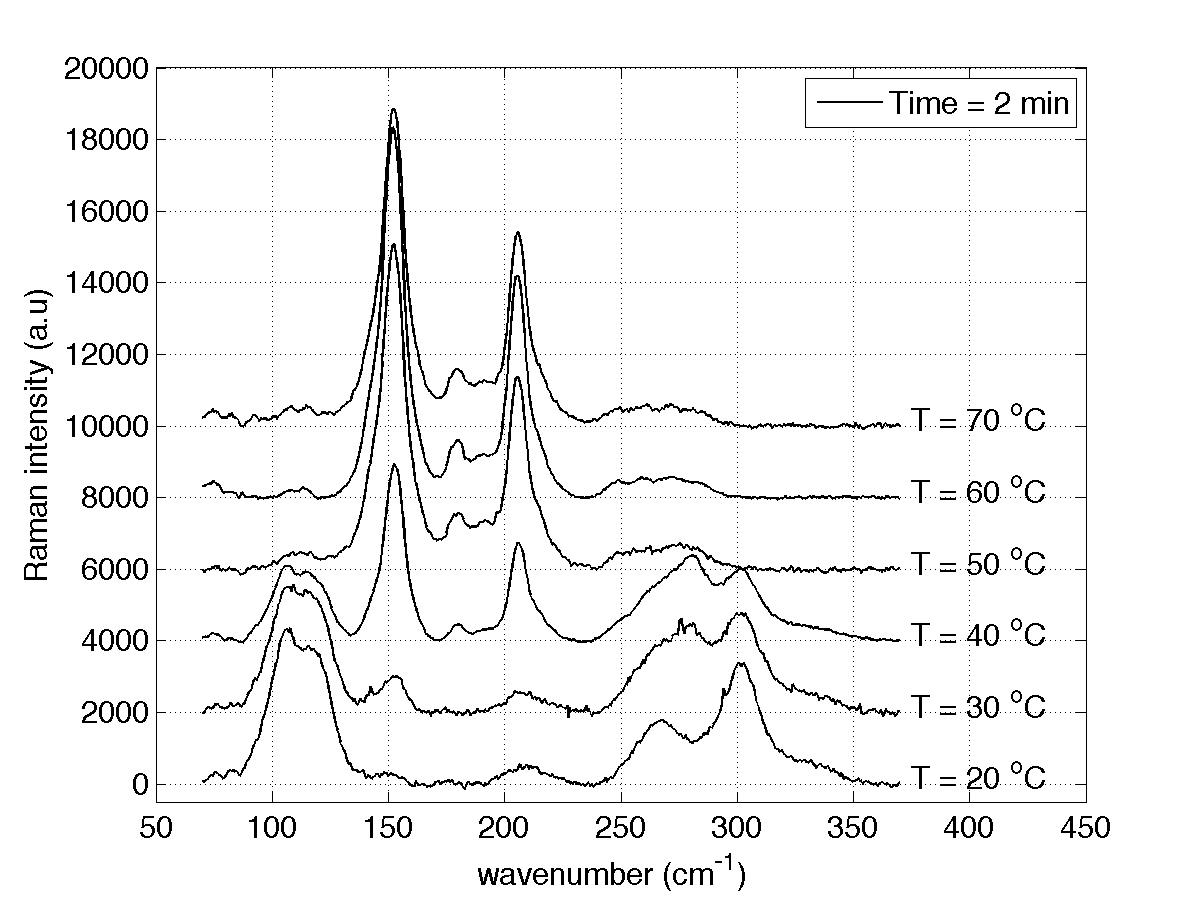
The Raman spectra of the polymorph mixture are firstly processed using a background removal approach proposed in [40]. In this method, the baseline is represented by a polynomial whose parameters are estimated by minimizing a truncated quadratic cost function. This method requires the specification of the polynomial order and the threshold of the quadratic cost function truncation. This method was applied for each spectrum separately with a fifth order polynomial and a threshold chosen by trial and error. Figure 7 shows the Raman spectra at the beginning of the phase transformation step, after background removal.

Figure 7: Mixture spectra at the beginning of the phase transformation.

VI-C Polymorph mixture separation under non-negativity and full additivity contraints

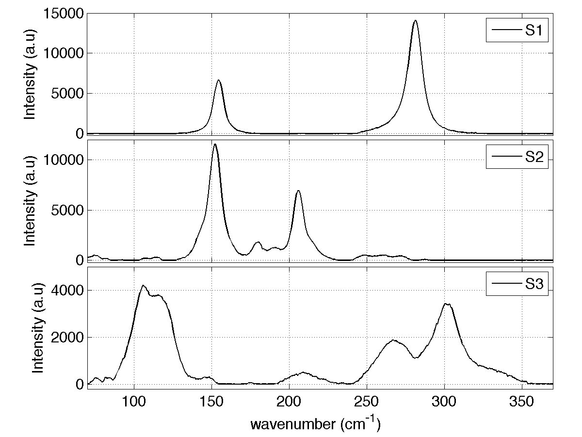
The number of sources to be recovered is fixed to $M=3$ according to the prior knowledge on the mixture composition. The iteration number is fixed to $1000$ iterations where the first $200$ samples are discarded since they correspond to the burn-in period of the Gibbs sampler. Figure 8 illustrates the estimated spectra using the proposed approach incorporating the non-negativity and the full additivitty constraints.

From a spectroscopic point of view and according to the positions of the vibrational peaks, the identification of the three components is very easy: the first source corresponds to Calcite, the second spectrum to Aragonite and the third one to Vaterite. A measure of the dissimilarity between the estimated spectra and the measured pure spectra of the three components gives $4.56$% for Calcite, $0.65$% for Aragonite and $4.76$% for Vaterite. These results show that the proposed method can be applied successfully without imposing any prior information on the shape of the pure spectra.

Figure 8: Estimated sources.

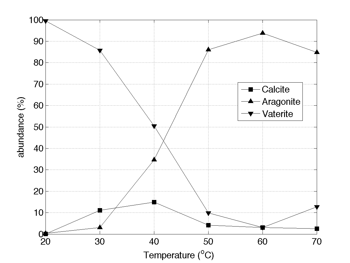
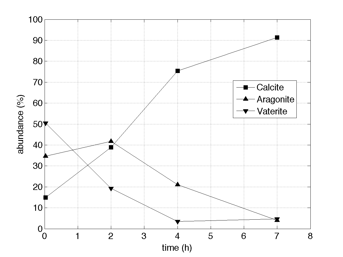
The evolution of the polymorph proportions versus temperature is shown in Fig. 9. Pure Vaterite is observed at $20$ C and a quite pure Aragonite is obtained at $60$ C. However, between $20$ C and $60$ C ternary mixtures are observed. The content of Calcite is maximal at $40$ C. Let us now consider the phase transformation evolution at this temperature value. The concentration profile versus precipitation time at 40 C is reported in figure 10. At the beginning of the phase transformation ($2$ minutes), the ternary mixture is composed of $50$% Vaterite, $35$% Aragonite and $15$% Calcite. After $2$ hours, the Vaterite is transformed to Aragonite and Calcite. After $7$ hours, Vaterite and Aragonite are almost totally transformed to calcite. So, aging time promotes the formation of Calcite which is in agreement with some results reported in the literature [41, 42].

Figure 9: Three component abundances at the beginning of the phase transformation for different temperature values.

Figure 10: Evolution of the three component abundances for $T=40$ C.

VI-D Polymorph Mixture analysis using other BSS algorithms

The dataset resulting from this experiment is also used to compare the performances of standard BSS methods taking into account the non-negativity constraint and their re-scaled versions ensuring the full additivity constraint. Table IV summarizes the performances of the considered separation algorithms in terms of normalized mean square errors, dissimilarity measures and computation times. It can be noticed that the proposed approach provides source estimates with better accuracy than the other methods. In addition to the good estimation quality, the second advantage of the proposed method is its ability to scale the sources during the estimation algorithm. Thus it does not require any post-processing of the estimation results. However, as previously highlighted, the price to pay for having such results is the computational times required by the proposed MCMC-based estimation method.

TABLE IV: Estimation performance for different BSS algorithms on real spectroscopic data.

	$\mathrm{NMSE}(\mathbf{S})$	$\mathrm{Diss}(\mathbf{S})$	Time (sec)
Proposed approach	0.0072	3.34	146
BPSS	0.0118	4.87	205
re-scaled-BPSS	0.0124	4.87	205
NNICA	0.1007	11.82	29
re-scaled NNICA	0.3996	11.82	29
NMF	0.0093	4.25	26
re-scaled NMF	0.0109	4.25	26

VII Conclusion

This paper studied Bayesian algorithms for separating linear mixtures of spectral sources under non-negativity and full additivity constraints. These two constraints are required in some applications such as hyperspectral imaging and spectroscopy to get meaningful solutions. A hierarchical Bayesian model was defined based on priors ensuring the fulfillment of the constraints. Estimation of the sources as well as the mixing coefficients was then performed by using samples distributed according to the joint posterior distribution of the unknown model parameters. A Gibbs sampler strategy was proposed to generate samples distributed according to the posterior of interest. The generated samples were then used to estimate the unknown parameters. The performance of the algorithm was first illustrated by means of simulations conducted on synthetic signals. The application to the separation of chemical mixtures resulting from Raman spectroscopy was finally investigated. The proposed Bayesian algorithm provided very promising results for this application. Particularly, when the computational times is not a study constraint, the proposed method clearly outperforms other standard NMF techniques, which can give approximative solutions faster. Perspectives include the development of a similar methodology for unmixing hyperspectral images. Some results were already obtained for the unmixing of known sources. However, the joint estimation of the mixing coefficients (abundances) and the sources (endmembers) is a still an open and challenging problem.

References

- [1] A. Cichocki and S.-I. Amari, Adaptive blind signal and image processing – Learning algorithms and applications. Chichester, England: John Wiley & Sons, 2002.
- [2] P. Comon, C. Jutten, and J. Hérault, “Blind separation of sources, Part II: Problems statement,” Signal Processing, vol. 24, no. 1, pp. 11–20, July 1991.
- [3] P. Comon, “Independent component analysis – a new concept?” Signal Processing, vol. 36, no. 3, pp. 287–314, April 1994.
- [4] J.-F. Cardoso, “Blind signal separation: statistical principles,” Proc. IEEE, vol. 9, no. 10, pp. 2009–2025, Oct. 1998.
- [5] A. Hyvärinen, J. Karhunen, and E. Oja, Independent Component Analysis. New York: John Wiley, 2001.
- [6] M. D. Plumbley, “Algorithms for non-negative independent component analysis,” IEEE Transactions on Neural Networks, vol. 14, no. 3, pp. 534–543, May 2003.
- [7] P. Sajda, S. Du, T. R. Brown, R. Stoyanova, D. C. Shungu, X. Mao, and L. C. Parra, “Nonnegative matrix factorization for rapid recovery of constituent spectra in magnetic resonance chemical shift imaging of the brain,” IEEE Trans. Medical Imaging, vol. 23, no. 12, pp. 1453–1465, 2004.
- [8] S. Moussaoui, D. Brie, A. Mohammad-Djafari, and C. Carteret, “Separation of non-negative mixture of non-negative sources using a Bayesian approach and MCMC sampling,” IEEE Trans. Signal Processing, vol. 54, no. 11, pp. 4133–4145, Nov. 2006.
- [9] P. O. Hoyer, “Non-negative matrix factorization with sparseness constraints,” Journal of Machine Learning Research, vol. 5, pp. 1457–1469, Dec. 2004.
- [10] C. Févotte and S. J. Godsill, “A Bayesian approach for blind separation of sparse sources,” IEEE Trans. Audio, Speech, Language Processing, vol. 14, no. 6, pp. 2174–2188, Nov. 2006.
- [11] H. Snoussi and J. Idier, “Bayesian blind separation of generalized hyperbolic processes in noisy and underdeterminate mixtures,” IEEE Trans. Signal Processing, vol. 54, no. 9, pp. 3257 – 3269, Sept. 2006.
- [12] E. R. Malinowski, Factor Analysis in Chemistry, 3rd ed. New York: John Wiley & Sons, 2002.
- [13] C.-I Chang, Hyperspectral Data Exploitation: theory and applications. Hoboken, NJ: John Wiley & Sons, 2007.
- [14] N. Dobigeon, J.-Y. Tourneret, and A. O. Hero, “Bayesian linear unmixing of hyperspectral images corrupted by colored Gaussian noise with unknown covariance matrix,” in Proc. IEEE Int. Conf. Acoust., Speech, and Signal (ICASSP), Las Vegas, Nevada, USA, March 2008.
- [15] A. de Juan, E. Casassas, and R. Tauler, “Soft-modelling of analytical data,” in Wiley encyclopedia of analytical chemistry: instrumentation and applications, ser. Soft-modelling of analytical data. Wiley Interscience, 2000, vol. 11, pp. 9800–9837.
- [16] N. Dobigeon, J.-Y. Tourneret, and C.-I Chang, “Semi-supervised linear spectral unmixing using a hierarchical Bayesian model for hyperspectral imagery,” IEEE Trans. Signal Processing, vol. 56, no. 7, pp. 2684–2695, July 2008.
- [17] D. D. Lee and H. S. Seung, “Learning the parts of objects by non-negative matrix factorization,” Nature, vol. 401, pp. 788–791, 1999.
- [18] I.-T. Hsiao, A. Rangarajan, and G. Gindi, “Bayesian image reconstruction for transmission tomography using mixture model priors and deterministic annealing algorithms,” Journal of Electronic Imaging, vol. 12, no. 1, pp. 7–16, 2003.
- [19] J. Miskin and D. MacKay, “Ensemble learning for blind source separation,” in S. Roberts and R. Everson, editors, Independent Component Analysis: Principles and Practice. Cambridge University Press, 2001, pp. 209–233.
- [20] N. Dobigeon, S. Moussaoui, and J.-Y. Tourneret, “Blind unmixing of linear mixtures using a hierarchical Bayesian model. Application to spectroscopic signal analysis,” in Proc. IEEE/SP Workshop Stat. Signal Processing, Madison, USA, Aug. 2007, pp. 79–83.
- [21] C. P. Robert, The Bayesian Choice: from Decision-Theoretic Motivations to Computational Implementation, 2nd ed., ser. Springer Texts in Statistics. New York, NY, USA: Springer-Verlag, 2007.
- [22] C. M. Bishop, Pattern Recognition and Machine Learning. New York: Springer, 2006.
- [23] E. Punskaya, C. Andrieu, A. Doucet, and W. Fitzgerald, “Bayesian curve fitting using MCMC with applications to signal segmentation,” IEEE Trans. Signal Processing, vol. 50, no. 3, pp. 747–758, March 2002.
- [24] C. P. Robert and G. Casella, Monte Carlo Statistical Methods. New York: Springer-Verlag, 1999.
- [25] C. P. Robert, “Simulation of truncated normal variables,” Statistics and Computing, vol. 5, no. 2, pp. 121–125, June 1995.
- [26] N. Dobigeon and J.-Y. Tourneret, “Efficient sampling according to a multivariate Gaussian distribution truncated on a simplex,” IRIT/ENSEEIHT/TéSA, Tech. Rep., March 2007. [Online]. Available: http://dobigeon.perso.enseeiht.fr/publis.html
- [27] J. Geweke, “Efficient simulation from the multivariate normal and Student-T distributions subject to linear constraints,” in Computing Science and Statistics, Proc. of the 23th Symposium on the Interface, E. M. Keramidas, Ed. Fairfax, VA: Interface Foundation of North America, Inc., 1991, pp. 571–578.
- [28] V. Mazet, D. Brie, and J. Idier, “Simulation of postive normal variables using several proposal distributions,” in Proc. IEEE Workshop on Statistical Signal Processing (SSP), Bordeaux, France, July 2005, pp. 37–42.
- [29] A. Gelman and D. B. Rubin, “Inference from iterative simulation using multiple sequences,” Statistical Science, vol. 7, no. 4, pp. 457–511, 1992.
- [30] P. M. Djurić and J.-H. Chun, “An MCMC sampling approach to estimation of nonstationary hidden Markov models,” IEEE Trans. Signal Processing, vol. 50, no. 5, pp. 1113–1123, 2002.
- [31] N. Dobigeon, J.-Y. Tourneret, and J. D. Scargle, “Joint segmentation of multivariate astronomical time series: Bayesian sampling with a hierarchical model,” IEEE Trans. Signal Processing, vol. 55, no. 2, pp. 414–423, Feb. 2007.
- [32] N. Dobigeon, J.-Y. Tourneret, and M. Davy, “Joint segmentation of piecewise constant autoregressive processes by using a hierarchical model and a Bayesian sampling approach,” IEEE Trans. Signal Processing, vol. 55, no. 4, pp. 1251–1263, April 2007.
- [33] S. Godsill and P. Rayner, “Statistical reconstruction and analysis of autoregressive signals in impulsive noise using the Gibbs sampler,” IEEE Trans. Speech, Audio Proc., vol. 6, no. 4, pp. 352–372, 1998.
- [34] A. Gelman, J. B. Carlin, H. S. Stern, and D. B. Rubin, Bayesian Data Analysis. London: Chapman & Hall, 1995.
- [35] C. P. Robert and S. Richardson, “Markov Chain Monte Carlo methods,” in Discretization and MCMC Convergence Assessment, C. P. Robert, Ed. New York: Springer Verlag, 1998, pp. 1–25.
- [36] M. D. Plumbley and E. Oja, “A nonnegative PCA algorithm for independent component analysis,” IEEE Trans. Neural Networks, vol. 15, no. 1, pp. 66–76, Jan. 2004.
- [37] J. K. Tugnait, “Identification and deconvolution of multichannel linear non-Gaussian processes using higher order statistics and inverse filter criteria,” IEEE Trans. Signal Processing, vol. 45, no. 3, pp. 658–672, March 1997.
- [38] S. Moussaoui, C. Carteret, D. Brie, and A. Mohammad-Djafari, “Bayesian analysis of spectral mixture data using Markov chain Monte Carlo methods,” Chemometrics and Intelligent Laboratory Systems, vol. 81, no. 2, pp. 137–148, April 2006.
- [39] C. Carteret, A. Dandeu, S. Moussaoui, H. Muhr, B. Humbert, and E. Plasari, “Polymorphism studied by lattice phonon raman spectroscopy and statistical mixture analysis method. Application to calcium carbonate polymorphs during batch crystallization,” Crystal Growth & Design, vol. 9, no. 2, pp. 807–812, 2009.
- [40] V. Mazet, C. Carteret, D. Brie, J. Idier, and B. Humbert, “Background removal from spectra by designing and minimising a non-quadratic cost function,” Chemometrics and Intelligent Laboratory Systems, vol. 76, no. 2, pp. 121–133, April 2005.
- [41] M. J. Kitamura, “Controlling factor of polymorphism in crystallization process,” J. Cryst. Growth, vol. 237, pp. 2205–2214, 2002.
- [42] A. Dandeu, B. Humbert, C. Carteret, H. Muhr, E. Plasari, and J.-M. Bossoutrot, “Raman spectroscopy - a powerful tool for the quantitative determination of the composition of polymorph mixtures: Application to CaCO3 polymorph mixtures,” Chem. Eng. Tech., vol. 29, no. 2, pp. 221–225, 2006.