The coming of age of X-ray polarimetry

Abstract

We review the polarization properties of X-ray emission from highly magnetized neutron stars, focusing on emission from the stellar surfaces. We discuss how x-ray polarization can be used to constrain neutron star magnetic field and emission geometry, and to probe strong-field quantum electrodynamics and possibly constrain the properties of axions.

Chapter 0 Polarized X-rays from Magnetized Neutron Stars

1 Introduction

One of the most important advances in neutron star (NS) astrophysics in the last decade has been the detection and detailed studies of surface (or near-surface) X-ray emission from a variety of isolated NSs kaspi06 ; harding06 . This has been made possible by X-ray telescopes such as Chandra and XMM-Newton. Such studies can potentially provide invaluable information on the physical properties and evolution of NSs (e.g., equation of state at super-nuclear densities, cooling history, surface magnetic fields and compositions, different NS populations). The inventory of isolated NSs with detected surface emission includes: (i) Radio pulsars: e.g., the phase-resolved spectroscopic observations of the “three musketeers” revealed the geometry of the NS polar caps; (ii) Magnetars (AXPs and SGRs): e.g., the quiscent emission of magnetars consists of a blackbody at $T\sim 0.5$ keV with a power-law component (index 2.7-3.5), plus significant emission up to $\sim 100$ keV; (iii) Central Compact Objects (CCOs) in SNRs: these now include 6-8 sources, several have $P,{\dot{P}}$ measurements and two have absorption lines deluca08 ; (iv) Thermally-Emitting Isolated NSs: these are a group of 7 nearby ($\mathrel{\raise 1.29167pt\hbox{$<$}\mkern-14.0mu\lower 2.58334pt\hbox{$\sim$}}1$ kpc) NSs with low ($\sim 10^{32}$ erg s^-1) X-ray luminosities and long (3-10 s) spin periods, and recent observations have revealed absorption features in many of the sources vankerkwijk07 ; kaplan08

In the coming decade, the most important goals in NS astrophysics include: (i) understanding how these different types of NSs evolve and relate to each others; (ii) elucidating the different observational manifestations (e.g., radiative processes in NS atmospheres and magnetospheres); (iii) using NSs to probe physics under extreme conditions. An obvious message of this paper is that in addition to imaging, timing and spectroscopy, X-ray polarimetry provides a window to study NSs: e.g., even when the spectrum or light curve is “boring”, polarization can still be interesting and very informative. Recent advances in detector technology suggest that polarimetry study of X-ray sources holds great promise in the future (see contributions by E. Costa, J. Swank, and M. Weiskopf in this proceedings).

2 Polarized X-rays from NSs: Basics

The surface emission from magnetized NSs (with $B\mathrel{\raise 1.29167pt\hbox{$>$}\mkern-14.0mu\lower 2.58334pt\hbox{$\sim$}}10^{12}$ G) is highly polarized gnedin74 ; pavlov00 for the following reason. In the magnetized plasma that characterizes NS atmospheres, X-ray photons propagate in two normal modes: the ordinary mode (O-mode, or $\parallel$-mode) is mostly polarized parallel to the ${\bf k}$-${\bf B}$ plane, while the extraordinary mode (X-mode, or $\perp$-mode) is mostly polarized perpendicular to the ${\bf k}$-${\bf B}$ plane, where ${\bf k}$ is the photon wave vector and ${\bf B}$ is the external magnetic field. This description of normal modes applies under typical conditions, when the photon energy $E$ is much less than the electron cyclotron energy $E_{Be}=\hbar eB/(m_{e}c)=11.6\,B_{12}$ keV [where $B_{12}=B/(10^{12}\,{\rm G})$], $E$ is not too close to the ion cyclotron energy $E_{Bi}=6.3\,B_{12}(Z/A)$ eV (where $Z$ and $A$ are the charge number and mass number of the ion), the plasma density is not too close to the vacuum resonance (see below) and $\theta_{B}$ (the angle between ${\bf k}$ and ${\bf B}$) is not close to zero. Under these conditions, the X-mode opacity (due to scattering and absorption) is greatly suppressed compared to the O-mode opacity, $\kappa_{X}\sim(E/E_{Be})^{2}\kappa_{O}$. As a result, the X-mode photons escape from deeper, hotter layers of the NS atmosphere than the O-mode photons, and the emergent radiation is linearly polarized to a high degree pavlov00 ; ho01 ; ho03 ; vanadelsberg06 . Thus, if we were to put a polarimeter on the NS surface we would measure high-polarization X-rays.

To translate this “surface measurement” into the observed signals at infinity, we need to understand how a photon (including its polarization state) evolves as it travels from the emission point to the observer. This will involve considering the geometry of the emission region (including magnetic field), light bending, and polarization evolution. Before discussing these issues, we summarize some of the general expected X-ray polarization characteristics:

(i) The X-ray polarization vector is either $\perp$ or $\parallel$ to the ${\bf k}$-$\mu$ plane, depending on the photon energy and surface field strength, even when the surface field is non-dipole! (Here $\mu$ is the magnetic dipole axis.)

(ii) As the NS rotates, we will obtain a “linear polarization sweep” (as in the rotating vector model of radio pulsars). This will provide a constraint on the dipole magnetic field geometry.

Thus, measurements of X-ray polarization, particularly when phase-resolved and measured in different energy bands, could provide unique constraints on the NS magnetic field (both the dipole component and the “total” strength) and geometry. There is only a modest dependence on $M/R$ of the NS, but as we discuss in the next section, quantum electrodynamics (QED) plays an important role.

Other Issues: (i) For sufficiently low $T$ and high $B$, there is a possibility that the NS surface is in a condensed (metallic) form, with negligible “vapor” above it medin07 . This has been suggested in the case of the TINS RX J1856.5-3754 vankerkwijk07 ; ho07 . Radiation from a condensed surface is certainly quite different from an atmosphere, with distinct X-ray polarization characteristics vanadelsberg05 . (ii) In the case of magnetars, Compton scatterings by mildly relativistic e^± in the NS magnetosphere/corona are important in determining the X-ray spectra at $E\mathrel{\raise 1.29167pt\hbox{$>$}\mkern-14.0mu\lower 2.58334pt\hbox{$\sim$}}2$ keV fernandez07 ; nobili08 . How such scatterings affect the polarization signals of surface emission has not been studied.

3 QED Effects on X-ray Polarization Signals

It has long been predicted from quantum electrodynamics (QED) that in a strong magnetic field the vacuum becomes birefringent adler71 ; heyl97 . While this vacuum polarization effect makes the photon index of refraction deviate from unity only when $B\mathrel{\raise 1.29167pt\hbox{$>$}\mkern-14.0mu\lower 2.58334pt\hbox{$\sim$}}300B_{\rm Q}$, where $B_{\rm Q}=m_{e}^{2}c^{3}/(e\hbar)=4.414\times 10^{13}$ G is the critical QED field strength, it can significantly affect the spectra of polarization signals from magnetic NSs in more subtle way, at much lower field strengths In particular, the combined effects of vacuum polarization and magnetized plasma gives rise to a “vacuum resonance”: a photon may convert from the high-opacity mode to the low-opacity one and vice verse when it crosses the vacuum resonance region in the inhomogeneous NS atmosphere lai02 . For $B\mathrel{\raise 1.29167pt\hbox{$>$}\mkern-14.0mu\lower 2.58334pt\hbox{$\sim$}}7\times 10^{13}$ G (see below), this vacuum resonance phenomenon tends to soften the hard spectral tail due to the non-greyness of the atmospheric opacities and suppress the width of absorption lines, while for $B\mathrel{\raise 1.29167pt\hbox{$<$}\mkern-14.0mu\lower 2.58334pt\hbox{$\sim$}}7\times 10^{13}$ G, the spectrum is unaffected ho03 ; ho04 ; lai03a ; lai03b ; vanadelsberg06 .

The QED-induced vacuum birefringence influences the X-ray polarization signals from magnetic NSs in two ways. (i) Photon mode conversion in the NS atmosphere: Since the mode conversion depends on photon energy and magnetic field strength, this vacuum resonance effect gives rise to a unique energy-dependent polarization signal in X-rays: For “normal” field strengths ($B\mathrel{\raise 1.29167pt\hbox{$<$}\mkern-14.0mu\lower 2.58334pt\hbox{$\sim$}}7\times 10^{13}$ G), the plane of linear polarization at the photon energy $E\mathrel{\raise 1.29167pt\hbox{$<$}\mkern-14.0mu\lower 2.58334pt\hbox{$\sim$}}1$ keV is perpendicular to that at $E\mathrel{\raise 1.29167pt\hbox{$>$}\mkern-14.0mu\lower 2.58334pt\hbox{$\sim$}}4$ keV, while for “superstrong” field strengths ($B\mathrel{\raise 1.29167pt\hbox{$>$}\mkern-14.0mu\lower 2.58334pt\hbox{$\sim$}}7\times 10^{13}$ G), the polarization planes at different energies coincide lai03b ; vanadelsberg06 . (ii) Polarization mode decoupling in the magnetosphere: The birefringence of the magnetized QED vacuum decouples the photon polarization modes, so that as a polarized photon leaves the NS surface and propagates through the magnetosphere, its polarization direction follows the direction of the magnetic field up to a large radius (the so-called polarization limiting radius). The result is that although the magnetic field orientations over the NS surface may vary widely, the polarization directions of the photon originating from different surface regions tend to align, giving rise to large observed polarization signals heyl02 ; vanadelsberg06 ; wang09 .

1 QED Effect in NS Atmospheres

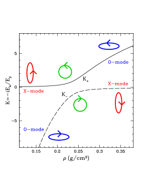
Figure 1: Vacuum resonance in a NS atmospheres: The polarization ellipticities of the two photon modes are shown as a function of density, for $B=10^{13}$ G, $E=5$ keV, $Y_{e}=1$ and $\theta_{B}=45^{\circ}$.

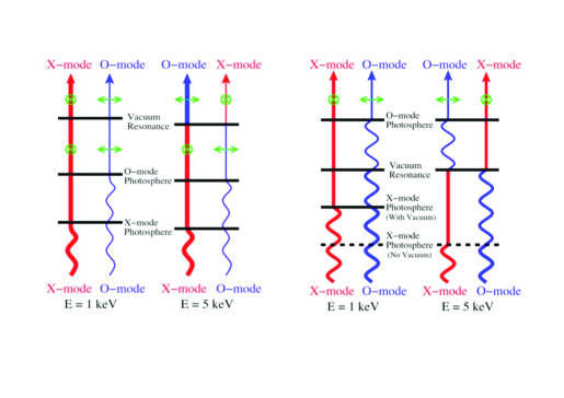
Figure 2: A schematic diagram illustrating how vacuum polarization affects the polarization state of the emergent radiation from a magnetized NS atmosphere. The left panel is for $B\mathrel{\raise 1.29167pt\hbox{$<$}\mkern-14.0mu\lower 2.58334pt\hbox{$\sim$}}B_{l}\simeq 7\times 10^{13}$ G, and the right panel for $B\mathrel{\raise 1.29167pt\hbox{$>$}\mkern-14.0mu\lower 2.58334pt\hbox{$\sim$}}B_{l}$. The photosphere is defined where the optical depth (measured from outside) is $2/3$.

In a magnetized NS atmosphere, both the plasma and vacuum polarization contribute to the dielectric tensor of the medium gnedin78 ; meszaros79 . The vacuum polarization contribution is of order $10^{-4}(B/B_{Q})^{2}f(B)$ (where $f\sim 1$ is a slowly varying function of $B$), and is quite small unless $B\gg B_{Q}$. The plasma contribution depends on $(\omega_{p}/\omega)^{2}\propto\rho/E^{2}$. The “vacuum” resonance arises when the effects of vacuum polarization and plasma on the polarization of the photon modes “compensate” each other. For a photon of energy $E$ (in keV), the vacuum resonance occurs at the density

$$\rho_{V}\simeq 0.964\,Y_{e}^{-1}B_{14}^{2}E^{2}f^{-2}~{}{\rm g~{}cm}^{-3},$$ (1)

where $Y_{e}$ is the electron fraction lai02 . Note that $\rho_{V}$ lies in the range of the typical densities of a NS atmosphere. For $\rho\mathrel{\raise 1.29167pt\hbox{$>$}\mkern-14.0mu\lower 2.58334pt\hbox{$\sim$}}\rho_{V}$ (where the plasma effect dominates the dielectric tensor) and $\rho\mathrel{\raise 1.29167pt\hbox{$<$}\mkern-14.0mu\lower 2.58334pt\hbox{$\sim$}}\rho_{V}$ (where vacuum polarization dominates), the photon modes are almost linearly polarized — they are the usual O-mode and X-mode described above; at $\rho=\rho_{V}$, however, both modes become circularly polarized as a result of the “cancellation” of the plasma and vacuum polarization effects (Fig. 1). When a photon propagates outward in the NS atmosphere, its polarization state will evolve adiabatically if the plasma density variation is sufficiently gentle. Thus the photon can convert from one mode into another as it traverses the vacuum resonance. For this conversion to be effective, the adiabatic condition must be satisfied:

$$E\mathrel{\raise 1.29167pt\hbox{$>$}\mkern-14.0mu\lower 2.58334pt\hbox{$\sim$}}E_{\rm ad}=1.49\,\bigl{(}f\,\tan\theta_{B}|1-u_{i}|\bigr{)}^{2/3}\left({5\,{\rm cm}/H_{\rho}}\right)^{1/3}~{}{\rm keV},$$ (2)

where $\theta_{B}$ is the angle between ${{\bf k}}$ and ${{\bf B}}$, $u_{i}=(E_{Bi}/E)^{2}$ ($E_{Bi}$ is the ion cyclotron energy), and $H_{\rho}=|ds/d\ln\rho|$ is the density scale height (evaluated at $\rho=\rho_{V}$) along the ray. For a typical atmosphere density scale height ($\sim 1$ cm), adiabatic mode conversion requires $E\mathrel{\raise 1.29167pt\hbox{$>$}\mkern-14.0mu\lower 2.58334pt\hbox{$\sim$}}1$-2 keV lai02 ; lai03a .

The location of vacuum resonance relative to the photospheres of X-mode and O-mode photons are important. For magnetic field strengths satisfying lai03a ; ho04

$$B\mathrel{\raise 1.29167pt\hbox{$>$}\mkern-14.0mu\lower 2.58334pt\hbox{$\sim$}}B_{l}\simeq 6.6\times 10^{13}\,T_{6}^{-1/8}E_{1}^{-1/4}S^{-1/4}\mbox{ G},$$ (3)

where $T_{6}=T/(10^{6}~{}{\rm K})$ and $S=1-e^{-E/kT}$, the vacuum resonance density lies between the X-mode and O-mode photospheres for typical photon energies, leading to suppression of spectral features and softening of the hard X-ray tail characteristic of the atmospheres. For “normal” magnetic fields, $B\mathrel{\raise 1.29167pt\hbox{$<$}\mkern-14.0mu\lower 2.58334pt\hbox{$\sim$}}B_{l}$, the vacuum resonance lies outside both photospheres, and the emission spectrum is unaltered by the vacuum resonance, although the observed polarization signals are still affected lai03b . See Fig. 2.

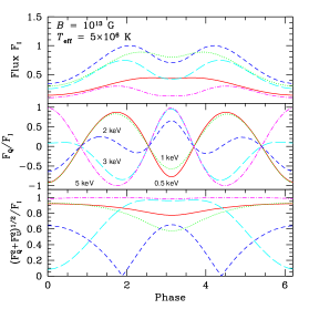
Figure 3: Lightcurve and polarization as a function of rotation phase for a NS hot spot with $B=10^{13}$ G, $T_{\rm eff}=5\times 10^{6}$ K. The angle of the spin axis relative to the line of sight is $\gamma=30^{\circ}$, and the inclination of the magnetic axis relative to the spin axis is $\eta=70^{\circ}$.

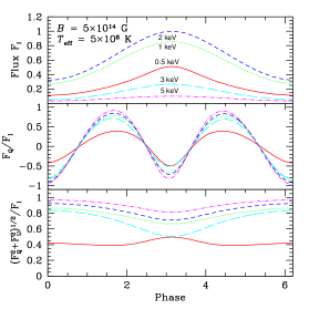
Figure 4: Same as Fig. 3, but for $B=5\times 10^{14}$ G.

Figures 3-4 give some examples of the polarization signal of a NS hot spot. We see that for $B\mathrel{\raise 1.29167pt\hbox{$<$}\mkern-14.0mu\lower 2.58334pt\hbox{$\sim$}}B_{l}$, the sign of the $F_{Q}$ Stokes parameter is opposite for low and high energy photons; this implies that the planes of polarization for low and high energy photons are perpendicular. For $B\mathrel{\raise 1.29167pt\hbox{$>$}\mkern-14.0mu\lower 2.58334pt\hbox{$\sim$}}B_{l}$, the planes of linear polarization at different $E$’s coincide. This is a unique signature of vacuum polarization.

2 QED Effect in Magnetospheres: Polarization Evolution

Consider radiation from a large patch of the NS, with ${\bf B}$ varying significantly across the emission region. Recall that locally at the NS surface, the emergent radiation is dominated by one of the two modes. If the photon polarization were parallel-transported to infinity, then the net polarization (summed over the observable patch of the NS) may be significantly reduced. However, this is incorrect heyl02 ; lai03b ; vanadelsberg06 . The reason is that, even in vacuum, the photon polarization modes are decoupled near the NS surface due to QED-induced birefringence, so that parallel-transport does not apply.

It is straightforward to obtain the observed polarized X-ray fluxes (Stokes parameters) from the fluxes at the emission region, at least approximately, without integrating the polarization evolution equations in the magnetosphere lai03b ; vanadelsberg06 . For a given (small) emission region of projected area (this is the area perpendicular to the ray at the emission point — General Relativistic light bending effect can be easily included in this), $\Delta A_{\perp}$, one need to know the intensities of the two photon modes at emission, $I_{\perp}$ and $I_{\parallel}$. In the case of thermal emission, these can be obtained directly from atmosphere/surface models. As the radiation propagates through the magnetosphere, the photon mode evolves adiabatically, following the variation of the magnetic field, until the polarization limiting radius $r_{\rm pl}$. This is where the two photon modes start recoupling to each other, and is determined by the condition $(\omega/c)\Delta n=2|d\phi_{B}/ds|$ (where $\Delta n$ is the difference of the indices of refraction of the two modes, $\phi_{B}$ specifies the direction of ${\bf B}$ along the ray), giving

$${r_{\rm pl}\over R_{\ast}}\simeq 70\left(E_{1}B_{\ast 13}^{2}P_{1}\right)^{1/6},$$ (4)

where $R_{\star}$ is the NS radius and $B_{\ast 13}$ is the polar magnetic field at the stellar surface in units of $10^{13}$ G [see ref. vanadelsberg06 for a more detailed expression). Beyond $r_{\rm pl}$, the photon polarization state is frozen. Thus the polarized radiation flux at $r\mathrel{\raise 1.29167pt\hbox{$>$}\mkern-14.0mu\lower 2.58334pt\hbox{$\sim$}}r_{\rm pl}$ is $F_{Q}=(I_{\parallel}-I_{\perp})\Delta A_{\perp}/D$, and $F_{U}\simeq F_{V}\simeq 0$, where $D$ is the distance of the source, $F_{Q}$ and $~{}F_{U}$ are defined in the coordinate system such that the stellar magnetic field at $r_{\rm pl}$ lies in the $XZ$ plane (with the $Z$-axis pointing towards the observer). Since $r_{\rm pl}$ is much larger than the stellar radius, the magnetic fields as “seen” by different photon rays are aligned and are determined by the dipole component of the stellar field, one can simply add up contributions from different surface emission areas to $F_{Q}$ to obtain the observed polarization fluxes.

Note that the description of the polarization evolution in the last paragraph is valid regardless of the possible complexity of the magnetic field near the stellar surface. This opens up the possibility of constraining the surface magnetic field of the neutron star using X-ray polarimetry. For example, the polarization light curve (particularly the dependence on the rotation phase) depends only on the dipole component of the magnetic field, while the intensity lightcurve of the same source depends on the surface magnetic field. On the other hand, the linear polarization spectrum (i.e., its dependence on the photon energy) depends on the magnetic field at the emission region lai03b ; vanadelsberg06 ; thus it is possible that a NS with a weak dipole field ($\mathrel{\raise 1.29167pt\hbox{$<$}\mkern-14.0mu\lower 2.58334pt\hbox{$\sim$}}7\times 10^{13}$ G) may exhibit X-ray polarization spectrum characteristic of a $B\mathrel{\raise 1.29167pt\hbox{$>$}\mkern-14.0mu\lower 2.58334pt\hbox{$\sim$}}7\times 10^{13}$ G NS.

One complication arises from Quasi-tangential (QT) effect: As the photon travels through the magnetosphere, it may cross the region where its wave vector is aligned or nearly aligned with the magnetic field (i.e., $\theta_{B}$ is zero or small). In such a QT region, the two photon modes ($\parallel$ and $\perp$ modes) become (nearly) identical, and can temporarily recouple, thereby affecting the polarization alignment wang09 . This QT effect gives rise to partial mode conversion: after passing through the QT point, the mode intensities change to ${\bar{I}}_{\parallel}\neq I_{\parallel}$ and ${\bar{I}}_{\perp}\neq I_{\perp}$. The observed polarization flux is then ${\bar{F}}_{Q}=({\bar{I}}_{\parallel}-{\bar{I}}_{\perp})\Delta A/D\neq F_{Q}$.

In the most general situations, to account for the QT propagation effect, it is necessary to integrate the polarization evolution equations in order to obtain the observed radiation Stokes parameters. However, Wang & Lai (2009) showed that for generic near-surface magnetic fields, the effective region where the QT effect leads to significant polarization changes covers only a small area of the neutron star surface. For a given emission model (and the size of the emission region) and magnetic field structure, Wang & Lai derived the criterion to evaluate the importance of the QT effect. In the case of surface emission from around the polar cap region of a dipole magnetic field, they quantified the effect of QT propagation in detail and provided a simple, easy-to-use prescription to account for the QT effect in determining the observed polarization fluxes. The net effect of QT propagation is to reduce the degree of linear polarization, so that ${\bar{F}}_{Q}/F_{Q}<1$, with the reduction factor depending on the photon energy, magnetic field strength, geometric angles, rotation phase and the emission area. The largest reduction is about a factor of two, and occurs for a particular emission size. Obviously, for emission from a large area of the stellar surface, the QT effect is negligible.

4 Probing Axions with Polarized X-Rays

The axion is a hypothesized pseudoscalar particle, introduced in 1980’s to explain the absence of strong CP violation. The axion is also an ideal candidate for cold dark matter, with the allowed axion mass $m_{a}$ is in the range of $10^{-6}\mathrel{\raise 1.29167pt\hbox{$<$}\mkern-14.0mu\lower 2.58334pt\hbox{$\sim$}}m_{a}\mathrel{\raise 1.29167pt\hbox{$<$}\mkern-14.0mu\lower 2.58334pt\hbox{$\sim$}}10^{-3}$ eV.

A general property of the axion is that it can couple to two photons (real or virtual) via the interaction

$${\cal L}_{a\gamma\gamma}=-{1\over 4}\,g\,a\,F_{\mu\nu}{\tilde{F}}^{\mu\nu}=g\,a\,{\bf E}\cdot{\bf B},$$ (5)

where $a$ is the axion field, $F_{\mu\nu}$ (${\tilde{F}}^{\mu\nu}$) is the (dual) electromagnetic field strength tensor, and $g$ is the photon-axion coupling constant. Accordingly, in the presence of a magnetic field, a photon (the $\parallel$ component) may oscillate into an axion and vice versa. Exploiting such photon-axion oscillation, various experiments and astrophysical considerations have been used to put constraint on the allowed values of $g$ and $m_{a}$ raffelt08 ; cast09 .

Magnetic NSs can serve as a useful laboratory to probe axion-photon coupling. Lai & Heyl (2006) presented the general methods for calculating the axion-photon conversion probability during propagation through a varying magnetized vacuum as well as across an inhomogeneous atmosphere. Partial axion-photon conversion may take place in the vacuum region outside the NS. Strong axion-photon mixing occurs due to a resonance in the atmosphere, and depending on the axion coupling strength and other parameters, significant axion-photon conversion can take place at the resonance. Such conversions may produce observable effects on the radiation spectra and polarization signals from the star. More study is needed in order to determine whether it is possible to separate out the photon-axion coupling effect from the intrinsic astrophysical uncertainties of the sources. See ref. lai06 for more details and references.

99

Adler, S.L. 1971, Ann. Phys., 67, 599

CAST collaboration, 2009, arXiv:0905.4273

De Luca, A. 2008, in 40 years of Pulsars: Millisecond Pulsars, Magnetars and More, eds. C. Bassa et al. (NY: AIP), 311

Fernandez, R., & Thompson, C. 2007, ApJ, 660, 615

Gnedin, Yu.N., Sunyaev R.A., 1974, A&A. 36, 379

Gnedin, Yu.N., Pavlov, G.G., & Shibanov, Yu.A. 1978, Sov. Astro. Lett. 4, 117

Harding, A.K., & Lai, D. 2006, Rept. Prog. Phys., 69, 2631

Heyl, J.S., & Hernquist, L. 1997, Phys. Rev. D55, 2449

Heyl, J.S., & Shaviv, N.J. 2002, Phys. Rev. D66, 023002

Ho, W.C.G., & Lai, D. 2001, MNRAS, 327, 1081-1096

Ho, W.C.G., & Lai, D. 2003, MNRAS, 338, 233

Ho, W.C.G., & Lai, D. 2004, ApJ, 607, 420

Ho, W.C.G., et al. 2007, MNRAS, 375, 821

Kaplan, D.L. 2008, in 40 years of Pulsars: Millisecond Pulsars, Magnetars and More, eds. C. Bassa et al. (NY: AIP), 331

Kaspi, V.M., Roberts, M., & Harding, A.K. 2006, in Compact Stellar X-ray Sources, eds. W. Lewin & M. van der Klis (Cambridge Univ. Press)

Lai, D., & Heyl, J. 2006, Phys. Rev. D74, 123003

Lai, D., & Ho, W.C.G. 2002, ApJ, 566, 373

Lai, D., & Ho, W.C.G. 2003a, ApJ, 588, 962

Lai, D., & Ho, W.C.G. 2003b, Phys. Rev. Lett. 91, 071101

Medin, Z., & Lai, D. 2007, MNRAS, 382, 1833

Mészáros, P. & Ventura, J. 1979, Phys. Rev. D 19, 3565

Nobili, L., Turolla, R., & Zane, S. 2008, MNRAS, 386, 1527

Pavlov, G.G. & Zavlin, V.E. 2000, ApJ, 529, 1011

Raffelt, G.G. 2008, Lect. Notes. Phys. 741, 51 (arXiv:hep-ph/0611350)

van Adelsberg, M., et al. 2005, ApJ, 628, 902

van Adelsberg, M., & Lai, D. 2006, MNRAS, 373, 1495

van Kerkwijk, M.H., & Kaplan, D.L. 2007, Ap&SS, 308, 191

Wang, C. & Lai, D. 2007, MNRAS, 377, 1095

Wang, C. & Lai, D. 2009, MNRAS, in press (arXiv:0903.2094)