The Connection Between Diffuse Light and Intracluster Planetary Nebulae in the Virgo Cluster

Abstract

We compare the distribution of diffuse intracluster light detected in the Virgo Cluster via broadband imaging with that inferred from searches for intracluster planetary nebulae (IPNe). We find a rough correspondence on large scales ($\sim$ 100 kpc) between the two, but with very large scatter ($\sim$ 1.3 mag/arcsec²). On smaller scales (1 – 10 kpc), the presence or absence of correlation is clearly dependent on the underlying surface brightness. On these scales, we find a correlation in regions of higher surface brightness ($\mu_{\mbox{V}}$$\;\buildrel<\over{\sim}\;$27) which are dominated by the halos of large galaxies such as M87, M86, and M84. In those cases, we are likely tracing PNe associated with galaxies rather than true IPNe. In true intracluster fields, at lower surface brightness, the correlation between luminosity and IPN candidates is much weaker. While a correlation between broadband light and IPNe is expected based on stellar populations, a variety of statistical, physical, and methodological effects can act to wash out this correlation and explain the lack of a strong correlation at lower surface brightness found here. A significant complication comes from the stochastic nature of the PN population combined with contamination of the IPN catalogs due to photometric errors and background emission line objects. If we attribute the lack of a strong observed correlation solely to the effects of contamination, our Monte Carlo analysis shows that our results are mostly consistent with a “IPNe-follow-light” model if the IPN catalogs are contaminated by $\sim$ 40%. Further complications arise from the line-of-sight depth of Virgo and uncertainty in the stellar populations of the ICL, both of which may contribute to the slight systematic differences seen between the IPN-inferred surface brightnesses and those derived from our deep surface photometry.

1. Introduction

The diffuse intracluster light (ICL) that permeates clusters of galaxies has become a valuable tool for studying galaxy cluster evolution. This ICL arises from a variety of sources, and is likely dominated by tidal stripping of galaxies during interactions both within the cluster and within infalling groups (Merritt 1984; Moore et al. 1996; Rudick, Mihos, & McBride 2006; Murante et al. 2008), as well as stripping by the cluster potential itself for galaxies passing near the cluster core (Byrd & Valtonen 1990; Gnedin 2003). Recent models of galaxy cluster accretion and evolution show that $\sim 10-40$% of the luminosity of clusters may be found in the ICL (e.g., Willman et al. 2004; Murante et al. 2004; Sommer-Larsen et al. 2005; Rudick et al. 2006; Purcell et al. 2007). Deep imaging of galaxy clusters has begun to reveal this ICL component (Bernstein et al. 1995; Feldmeier et al. 2002, 2004; Mihos et al. 2005; Zibetti et al. 2005; Gonzalez et al. 2005), with some suggestion of a correlation between cluster mass and ICL fraction (Ciardullo et al. 2004; Krick & Bernstein 2007).

Of particular interest is the dynamical information contained within the ICL. As material is stripped from its host galaxies, long tidal streams are formed (Gregg & West 1998; Calcáneo-Roldán et al. 2000; Feldmeier et al. 2004; Mihos et al. 2005); these coherent streams can later be destroyed during a subsequent cluster accretion event, contributing to a smooth diffuse ICL component (e.g., Rudick et al. 2006, 2008). The morphology of the diffuse ICL on cluster scales thus contains information on the recent accretion history of galaxy clusters. On smaller scales, the ICL can trace the dynamical history of individual galaxies, as extended tidal debris can highlight past interactions, either with the cluster potential or with other galaxies (e.g., Schweizer 1980; Malin 1994; Weil et al. 1997; Katsiyannis et al. 1998; Feldmeier et al. 2004; Janowiecki et al. in preparation).

Along with diffuse light, the ICL can be studied through discrete tracers such as globular clusters (West et al. 1995; Williams et al. 2007a), red giants (Ferguson, Tanvir, & von Hippel 1998; Durrell et al. 2002; Williams et al. 2007b), and planetary nebulae (Arnaboldi et al. 1996; Feldmeier et al. 1998, 2004; Aguerri et al. 2005). Intracluster planetary nebulae (IPNe) are of particular interest here, since they are believed to trace the stellar luminosity of galaxies and – as emission line objects – they permit study of the kinematics of the ICL. IPN kinematics have been studied in both the Virgo (Arnaboldi et al. 2004) and Coma (Gerhard et al. 2005) clusters, and yield interesting constraints on kinematic substructure. Larger samples of IPN velocities would yield information on the degree of relaxation of the ICL, its kinematic connection to the cluster galaxies, and also provide further constraints on the cluster mass distribution (Gerhard et al. 2007; Sommer-Larsen et al. 2005; Willman et al. 2005). However, existing surveys for IPNe have largely been done “blind,” without any of the foreknowledge of the underlying properties of the diffuse light provided by recent broadband imaging surveys (e.g., Mihos et al. 2005). A strong correlation between broadband light and IPN density would then open up the capability of using deep imaging to maximize the efficiency of followup IPN searches.

If well determined, the connection between planetary nebulae and broadband luminosity in the ICL also can provide constraints on its stellar populations. The ratio $\alpha=N_{\rm PNe}/L_{\rm bol}$ depends on the stellar populations of the ICL (see, e.g., Buzzoni, Arnaboldi, & Corradi 2006), and in galaxies shows a correlation with galaxy type (Peimbert 1990; Ciardullo et al. 2005), wherein massive metal-rich ellipticals have a much lower value of $\alpha$ than do low-luminosity, metal-poor galaxies. Measurements of $\alpha$ can test various models for the formation of the ICL, as ICL formed from the mergers of massive galaxies during the formation of a cluster (Murante et al. 2008) would show lower values of $\alpha$ than ICL formed from the ongoing disruption of low luminosity dwarfs orbiting in the cluster potential (Moore et al. 1996).

The data now exist to do this detailed comparison between the ICL measured by broad band light and IPNe in the Virgo Cluster. We (Mihos et al. 2005) have conducted a deep wide-field imaging survey of the Virgo core down to a $3\sigma$ limiting surface brightness of $\mu_{V}=28.5$, while narrowband surveys (Feldmeier et al. 2004; hereafter F04; Aguerri et al. 2005; hereafter A05) are discovering significant numbers of IPN candidates in Virgo. Many of these IPN fields overlap with our imaging fields, allowing us to do direct comparison between the different ICL tracers. These tracers have very different systematic uncertainties: broad band surface photometry is sensitive to sky subtraction, flat field quality, and scattered light control, while the IPN measurements rely on statistics of faint point source detection and contamination from background emission line objects. While the comparison will be complicated by these different systematic uncertainties, it also gives us a new opportunity to assess the consistency of the two methods in detecting the diffuse intracluster light in galaxy clusters.

2. Observational Data

2.1. Broad band imaging

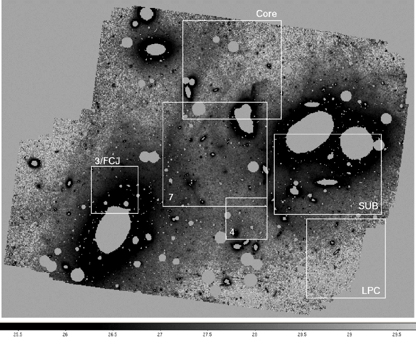
Figure 1.— Optical image of the Virgo cluster core, taken from Mihos et al. 2005. Intensity saturates black at a surface brightness of $\mu_{\mbox{V}}$=26.5, and the faintest ICL features visible have surface brightness $\mu_{\mbox{V}}$$\sim$ 28.5. The white masked areas represent either foreground stars or the inner regions of galaxies brighter than $\mu_{\mbox{V}}$=25. The various IPN fields from F04 (fields 3, 4, and 7) and A05 (FCJ, Core, SUB, and LPC) are overlaid.

The optical imaging comes from our ongoing survey for ICL in the Virgo cluster using the 0.6m Burrell Schmidt at Kitt Peak. Figure 1 shows our image of the central 2.5 square degrees of the Virgo core (see Mihos et al. 2005 for details). This image has been constructed from co-adding 72 individual 900s images, each dithered by up to half a degree. The dithering pattern means that the total exposure time across the field varies. The median number of exposures per pixel in the final mosaic is 31. The exposure time is highest in the inner 17% of the image, where there are at least 40 exposures per pixel; 73% of the pixels have at least 20 exposures, and the minimum exposure per pixel (which defines the edges of the mosaic) is set at 5. Each individual image was flattened using a night sky flat built from 127 offset sky pointings. The sky pointings were taken bracketing the Virgo images in both time and position, to minimize flat fielding variations due to telescope flexure and illumination. All images were taken in Washington M and transformed to Johnson V assuming a color of B-V=1 typical of the old stellar populations thought to represent intracluster light. The uncertainty in the ICL surface brightness introduced by the photometric transform is small – for example, adopting an extremely and unrealistically blue ICL color of B-V=0 changes the inferred surface brightness by only 0.18 magnitudes.

Sky subtraction is problematic when dealing with an image which subtends only a small fraction of the cluster area. To obtain an reliable estimate of sky, we first need to subtract the wings of bright stars from the image. We use long exposures of $\alpha$ Leo to construct the stellar point spread function out to 30′, and then subtract the extended wings of stars out a radius where they contribute 0.1 ADU ($\mu_{V}=30$) to the local sky. We also mask stars completely inside the radius where the scaled stellar PSF is brighter than 3 ADU. IRAF’s objmask task is then run on the star subtracted image to mask all extended sources 2.5$\sigma$ above a locally-measured sky value. The image is then spatially rebinned into “superpixels” which are 32x32 pixels in size; each superpixel is given an intensity equal to the mode of its individual pixels. Regions are then selected to represent “true sky” – these regions are chosen to be far from bright galaxies, and typically make up $\sim$ 15% of each individual image. For each image, an absolute sky value is then calculated from the mode of the superpixel intensities in these pure sky regions and subtracted off. Depending on varying airmass, time, and hour angle, these sky levels varied from 1100-1500 ADU ($\mu_{V}=21.6-21.3$).

To make the final mosaic, we then register each image and use the “true sky” regions to simultaneously and iteratively fit residual sky planes to the individual images, constrained to minimize the frame-to-frame deviations in overlapping regions of images. After registering and medianing the individual images into the final mosaic, one additional residual sky plane is fit and subtracted from the mosaic. It is important to note that this process will over-subtract any ICL which is smoothly distributed on scales larger than the areal coverage of the image, approximately 400 kpc on a side.

To construct the error model for the dataset, we follow the procedure outlined by Morrison et al. (1997), described in more detail in the Appendix. In brief, we expect a random error of approximately 2 ADU per pixel from a combination of readnoise, small-scale flat fielding errors, and sky photon noise. This uncertainty should become negligible when measuring the diffuse ICL over large scales ($>$30″), where many pixels contribute to the measurement. On these larger scales, however, the error model is dominated by uncertainty in the sky background and large scale flat-fielding, which we estimate to be approximately 0.5 ADU by examining the residual variance in boxes $2{\tt{}^{\prime}}\mskip-6.0mu.\,5$ on a side in regions lacking galaxies or diffuse light. This places the $3\sigma$ limiting depth to our surface photometry at $\mu_{V}=28.65$.

Table 1Virgo IPNe fields

Field	$m_{lim}$	$d_{lim}$	$N_{cand}$	$\mu_{\mbox{V}}$	Source		$\mu_{\mbox{V}}$(phot)		$N_{images}$
	(5007)	(Mpc)	$<m_{lim}$	(PNe)		$\mu_{\rm mask}$	$\mu_{\rm mask}$	$\mu_{\rm mask}$
		(a)		(b)		25.5	26	26.5	(c)
3	27.0	20.0	46	26.5	F04	26.4	26.7	27.0	35.3
4	26.6	16.6	4	27.4	F04	27.6	27.7	27.8	34.2
7	26.8	18.3	32	28.4	F04	27.2	27.3	27.5	45.1
Core	27.2	22.0	77	28.6	A05	27.8	27.9	28.1	35.2
FCJ	27.0	20.0	20	27.4	A05	26.4	26.7	27.0	35.3
LPC	27.5	25.2	14	31.7	A05	28.1	28.2	28.4	16.6
SUB	28.1	33.1	36	28.5	A05	26.6	26.9	27.3	37.7

2.2. IPN catalogs

We compare the broadband diffuse light measured in our Virgo imaging to that inferred from compilations of recent Virgo IPN surveys by F04 and A05. Catalogs for the latter datasets were kindly provided by Ortwin Gerhard and collaborators. These surveys were conducted on a variety of telescopes, have different areal coverage and selection effects, and go to different limiting magnitudes; combining these catalogs into a homogeneous dataset is problematic. Instead, our goal is to compare the IPN-inferred ICL surface brightnesses averaged over each field (§3), and then examine the correlation between individual IPN candidates and broadband light within individual fields (§4).

One major issue is that these catalogs are catalogs of IPN candidates detected via a two filter method. IPN candidates are identified as point sources that are present in a narrowband “on-band” image that includes the redshifted $\lambda$ 5007 [OIII] line, but disappears in a spectrally-adjacent “off-band” image that excludes the line. Unfortunately, such a search technique can also include contaminating objects, and the contamination in the IPN catalogs can be significant. This contamination comes in two forms. The first is background emission line objects, most notably high-redshift galaxies. At a redshift of $z=3.1$, Ly$\alpha$ falls into the narrowband [OIII] filters used to detect IPNe, such that a fraction of the IPN candidates are in fact background Ly$\alpha$ emitting galaxies. Estimates of this contamination fraction from narrowband imaging of blank fields (Ciardullo et al. 2002) put the fraction of background emitters at $\sim$ 20%. This fraction can vary significantly from field to field, however, depending on the fluctuations in the background distribution of the Ly$\alpha$ emitters. A second source of contamination can occur if the off-band image has a shallow limiting magnitude and joint photometric errors in the on-band and off-band images lead to sources being erroneously classified as emission-line objects (the so-called “spillover effect,” see A05). Combined, these effects can lead to significant contamination of the catalogs: Arnaboldi et al. (2004) have performed follow-up spectroscopy of IPN candidates in the FCJ, Core, and Sub fields, and achieve a confirmation rate of 84%, 32%, and 72%, respectively, for IPN candidates brighter than $m_{5007}=27.2$. We address the issue of contamination in more depth in §4 and §5.

A second concern is the uniqueness of the IPN candidate lists. Both the Field 3 and Field FCJ candidates were extracted from the same imaging dataset, but by two different groups using somewhat different methods for extracting the emission line candidates (see F04 and A05 for details). An examination of the candidates in the two fields shows markedly different samples. Of the 46 Field 3 and 19 FCJ candidates brighter than $m_{lim,5007}=27$, only 12 candidates are common to both catalogs. Spectroscopic follow-up of the FCJ candidates has been conducted by Arnaboldi et al. (2004), and the overlap of the spectroscopically-confirmed candidates is much better: 10/11 spectroscopically confirmed FCJ candidates also show up in the Field 3 catalog. Nonetheless, without full spectroscopic follow-up of all the IPN candidates in survey fields, we limit our analysis to the existing photometric IPN candidate lists.

With these caveats in mind, we show in Figure 2 the IPN candidates from F04 and A05 overlaid on the broadband image from Mihos et al. (2005). A visual examination of Figure 2 suggests that the correlation between PNe candidates and diffuse light depends on the underlying surface brightness – the connection is stronger near the luminous Virgo ellipticals, where their halo light dominates the fields, and weak or absent in regions of low surface brightness in truly intracluster fields. For example Field 3/FCJ, which is dominated by halo light from M87, shows a clear gradient in PNe density from the NE to the SW, along the direction of M87’s luminosity gradient. Many of these PNe are likely associated with M87 itself rather than being true intracluster PNe (see, e.g., the discussion in F04); indeed, followup spectroscopy of 15 IPN candidates in the FCJ field by Arnaboldi et al. (2004) shows that 12 of the 15 candidates have a narrow velocity distribution ($\sigma=247\pm 52$ km/s) that can be associated with M87’s halo. Similarly, the majority of IPN candidates in Field SUB are very clearly concentrated around the giant ellipticals M86 and M84.

In other fields further away from the luminous ellipticals and at much lower surface brightness, the correspondence between IPN candidates and broad band light is less clear. Field 4 only has four IPN candidates brighter than the limiting magnitude; it is hard to make any inferences about this field with so few candidates. Field 7 is more complex; there are candidate IPNe around the galaxy pair NGC 4435/8, as well as along the eastern edge of the field, where they may be associated with tidal streams coming from M87’s halo. In the Core field, there are many IPN candidates but no obvious connection to the galaxies. Field LPC is located in a region of our image that shows the least diffuse light, and indeed has only a small number of IPN candidates. If anything, however, these candidates appear anti-correlated with the broadband light, as they lie in the southwest (lower right) portion of the field while the M86/M84 complex lies just off the northeast (upper left) corner of the field.

As a comparison, we show in Figure 3 simulated PNe catalogs for each survey field, based on the assumption that PNe follow the broadband light detected in our deep imaging. To construct these catalogs, we build for each field a master PNe list under the assumption that the number of PNe in any given pixel is proportional to the pixel intensity ($N_{PNe}=C\times I_{i,j}$). To avoid PNe being assigned to noise spikes, the images are all median smoothed with a 9x9 pixel box before the IPN catalog is generated, and we do not generate PNe in regions of high surface brightness (at $\mu_{V}<25$ for all fields but SUB; in SUB, PNe candidates were found at higher surface brightness, and we choose the cutoff for this field to be $\mu_{V}<24$.) We choose the constant of proportionality $C$ so that a master list is generated of $O(10^{6})$ PNe, which ensures that master catalog contains potential IPN candidates even at low surface brightnesses. We then randomly select from this master catalog the same number of IPNe as found in the actual narrowband imaging data from F04 and A05. The random catalog shown in Figure 3 is typical of the catalogs generated this way.

Examining Figure 3, the connection between the ICL and the simulated IPNe is clearly stronger than in the real data. Many simulated PNe are found near the bright ellipticals in Fields 3, FCJ, and SUB, but now the correlation with NGC 4435/8 is much stronger in Fields 7 and Core. The simulated IPNe in the eastern (left) half of Field 7 more obviously lie on top of the M87 streams, and the simulated IPNe in Field LPC are concentrated in the northeast (upper left) portion of the image, towards the M86/M84 pair. The fact that these spatial biases are evident in the simulated dataset shows that the weaker bias seen in the real dataset is likely not simply a result of small number statistics.

Visually, therefore, the correlation between the IPN candidates and the diffuse broadband light is loose at best. In regions of higher surface brightness which encompass the extended halos of bright ellipticals – Field 3/FCJ and Core – the IPN candidates do seem to correlate with the galaxy light. At lower surface brightness in regions which are more truly intracluster, the results are more ambiguous – Field 7 suggests a possible correlation between the diffuse light and IPN candidates, but this not seen in Fields Core and LPC. Because of the lower surface brightness in the intracluster fields, much of this lack of correlation may be due to fractional contamination being higher in these fields. Furthermore, other factors may contribute as well to wash out the correlation, such as the depth of the Virgo Cluster causing IPNe on the far side of Virgo to be lost from the magnitude-limited IPN samples, or systematic variations in the value of $\alpha$ across Virgo. We address each of these possibilities in more detail below. However, because visual impressions are easily misled by the eye’s desire to find patterns in the data, we first must develop a more quantitative measure of the correlation between IPNe and the diffuse light.

Ideally, one could do this comparison by combining the various IPN catalogs into a single master catalog, and calculating the surface density of IPN candidates in regions of a given surface brightness across the cluster as whole. Unfortunately, this test is problematic for a number of reasons – one being the heterogeneity of the existing IPN datasets. Because the datasets all have different limiting magnitudes, contamination fractions, and selection criteria, we cannot combine them together to generate a homogeneous ”master list” of IPN candidates on which to make the suggested test. For example, at a given surface brightness, the IPN counts in one field may be low compared to another simply because the first field did not go as deep. Alternatively, counts in one field could be high compared to another if the first field had more contaminants. In principle, while a homogeneous master catalog cannot be built, we could attempt the test within individual fields. Here, however, we are limited both by the small number of IPN candidates per field, and, at lower surface brightness, uncertainty in the absolute surface photometry due to sky subtraction.

In Fields 3/FCJ and SUB, however, we have a means to attempt this test in a somewhat more model-dependent fashion. These fields are dominated by the halos of the elliptical galaxies M87 (for Field 3/FCJ) and M84/M86 (for Field SUB), and using our deep imaging we can use IRAF’s ELLIPSE task to construct model luminosity profiles for these ellipticals (Janowiecki et al. in preparation). We then define the areas of the field covered by isophotes of a given surface brightness, and calculate the IPN surface density in these areas as a function of surface brightness. Since the isophotal models are spatially smooth and extend to high surface brightness, this should provide a demonstration of how well the IPN candidates follow the galaxy luminosity distribution. The results are presented in Figure 4, where the dotted line shows the expectation if PNe surface density follows the stellar light profile of the galaxies. The correlation between the galaxy light and PNe surface density is clear, reminiscent of other studies of the PNe distribution around luminous spheriods such as M104 (Ford et al. 1996) and NGC 5128 (Hui et al. 1993).

However, the analysis in Figure 4 only tests the correlation between IPN density and the light profile of the giant ellipticals. It does not probe truly intracluster regions at low surface brightness where the luminosity distribution is spatially complex, nor does it factor in the contribution of fainter galaxies which may lie in the field. To test the correlation between IPN candidates and diffuse light more generally in all the IPN survey fields, we need to employ an alternative set of quantitative tests to explore the correlation between IPN candidates and broad band light. First, in §3 we compare the absolute level of surface brightnesses measured by our deep imaging with that inferred from the IPNe surveys, averaged over each survey field. Then, in §4 we examine the relative excess of light around IPN candidates in individual fields. The first approach deals with the problems of heterogeneity in the ICL data by relying on the statistical corrections for completeness and contamination that F04 and A05 have adopted for their datasets, allowing us to make the proper absolute comparison between different survey fields. The second approach deals with the problems of systematic uncertainty in the surface brightness data by making a relative measure of flux excess rather than an absolute measurement of surface brightness. If IPNe faithfully trace the diffuse light, that should manifest as an excess of light in regions around IPN candidates, compared to randomly sampled regions throughout a given field.

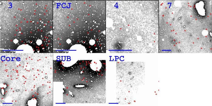
Figure 2.— IPN candidates from F04 and A05 overlaid on the broadband imaging from Mihos et al. (2005). Only candidates brighter than the limiting magnitude in each field (see Table 1) are shown. A 3′ scale bar is shown in the lower left of each field. The inner regions of galaxies are masked at $\mu_{\mbox{V}}$$<$25 mag/arcsec² for all fields except SUB, which is masked at $\mu_{\mbox{V}}$$<$24 mag/arcsec².

Figure 3.— Mock IPN catalogs overlaid on the broadband imaging from Mihos et al. (2005). The catalogs are generated under the assumption that PNe follow the broad band luminosity; see text for details. A 3′ scale bar is given at the bottom left of each field.The inner regions of galaxies are masked at $\mu_{\mbox{V}}$$<$25 mag/arcsec²for all fields except SUB, which is masked at $\mu_{\mbox{V}}$$<$24 mag/arcsec².

Figure 4.— IPN surface density versus modeled galaxy surface brightness near the ellipticals M87, M86, and M84. The surface brightness models are isophotal fits to the broad band imaging by Janowiecki et al. (in preparation). The dashed line shows the expectation if IPN surface density follows broadband surface brightness. The different limiting magnitudes and selection criteria for the different IPN datasets may lead to vertical offsets between the different curves, but the general trend that IPN surface density traces the light in the halos of the giant ellipticals seems clear.

3. Large Scale Averages: Absolute Measurements of ICL

We begin with an absolute comparison of the ICL measured in our deep broadband imaging to that inferred from the IPN measurements by F04 and A05 over larger scales (60–150 kpc). As discussed in §2, given the differences in the various IPN survey fields and catalog extraction techniques, combining the various IPN datasets is rather problematic. Rather than attempting to create a master IPN catalog, we adopt the analyses of F04 and A05, which convert IPN density to inferred broad-band surface brightness using statistical corrections for incompleteness and contamination which are appropriate to the individual survey fields. We also adopt a value of $\alpha$ ($=N_{\rm PNe}/L_{\rm bol}$) for the conversion which is standardized across all IPN fields (see below). This then gives us a measure of the absolute level of ICL in each survey field, which we can then compare to our own broadband imaging. We also note that the variation between the analysis by F04 and A05 of Field 3/FCJ can then be viewed as an estimate of the systematic uncertainty in the IPN-inferred surface brightness.

As mentioned previously, one needs to adopt a value for the parameter $\alpha$ to convert IPN counts to broadband surface brightness. The exact value of $\alpha$ depends on how far down the planetary nebular luminosity function (PNLF) one detects PNe, as well as the stellar population mix of the ICL (Buzzoni et al. 2006): more luminous, metal-rich galaxies have lower values of $\alpha$ than do low luminosity metal-poor systems (Ciardullo et al. 2005). For simplicity, we adopt IPN-inferred surface brightnesses calculated using the value of $\alpha$ determined from studies of individual intracluster stars in Virgo by Durrell et al. (2004), $\alpha_{2.5}=23^{+10}_{-12}\times 10^{-9}$ PNe/L$\sun$, where the “2.5” refers to the number of PNe 2.5 magnitudes below M*, the high-luminosity cutoff in the PNLF ($M*=-4.51$; Ciardullo et al. 2005). This relatively high value of $\alpha$ measured by Durrell et al. (2004) for the Virgo ICL is reflective of low luminosity systems ($M_{B}>-20.5$), but is measured only over a small field ($\sim$ 4 arcmin²) halfway between M87 and M86. Over the larger fields surveyed by the IPN surveys and our deep imaging, there may be significant and systematic differences in the stellar populations – and therefore the value of $\alpha$ – in Virgo’s ICL. We return to the uncertainty in $\alpha$ in §5 below.

We do make one more adjustment to the A05 analysis. A05 quote their inferred surface brightnesses in $\mu_{\mbox{B}}$, while both our imaging and the F04 results work in $\mu_{\mbox{V}}$. We therefore transform the A05 results from $\mu_{\mbox{B}}$ to $\mu_{\mbox{V}}$ by adopting a B-V color of 1.2, consistent with the choice of bolometric correction (BC=$-0.8$) adopted for the stellar populations in their work.

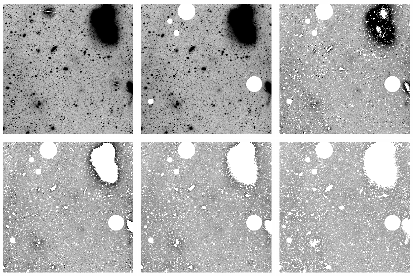
Figure 5.— The masking process applied to Field 7. The raw image is shown in the top left field. The top middle image show the image with the bright star mask. The SExtractor mask is added in the top right image. The bottom row shows the effects of adding a surface brightness mask, masking all pixels brighter than $\mu_{\mbox{V}}$=25.5 (left), $\mu_{\mbox{V}}$=26 (middle), and $\mu_{\mbox{V}}$=26.5 (right).

To measure the diffuse intracluster light in our fields, we must first mask out foreground stars and background galaxies (large, bright Virgo galaxies are handled in a separate step, described below). We mask using the prescription described in Feldmeier et al. (2002), and refer the reader there for more details; here we will walk briefly through the steps, using the Field 7 to illustrate the process (Figure 5). In brief, we start by manually masking all extremely bright stars, as well as their diffraction spikes and column bleeds (Figure 5b). We then run a ring median on the image and subtract off the ring median image from the raw image; producing an image where the large galaxies have essentially been removed. We use SExtractor (Bertin & Arnouts 1996) to identify sources on this median-subtracted image, using a very aggressive search: all objects 0.6$\sigma$ above sky and at least 3 pixels in size, creating a preliminary mask catalog which consists of both real objects and faint positive noise spikes.

We next need to filter the noise spikes out of the mask catalog, since masking only positive noise spikes, but not the corresponding negative noise spikes, would bias our final measurement of the ICL to artificially low values. We do this masking in a statistical sense, by multiplying the median-subtracted image by $-1$ to create a “negative image” and rerunning SExtractor with the same search parameters – the negative noise features it identifies should have the same distribution as the positive noise features in the original image, and we can use this distribution to statistically remove the noise features from the mask catalog. Specifically, as a function of source magnitude, we define a “noise fraction” (simply the ratio of the source counts detected in the negative image to those in the actual image) and then, for each source in the actual image, we use rejection sampling (based on the magnitude-dependent noise fraction) to determine whether or not to keep it in our final SExtractor masking catalog. We add this mask to the bright star mask to produce the second level of masking (Figure 5c).

The SExtractor mask does a good job of masking small galaxies and non-saturated stars, but as it is generated from a median-subtracted image, it fails to capture the large galaxies which disappear during a median subtraction. It also spuriously identifies as discrete sources bright spots (either real or noise) in the inner regions of galaxies. To overcome this, we add one last layer of masking, which masks out the high surface brightness regions of galaxies. This mask also qualitatively captures an areal selection effect wherein IPN studies generally do not concentrate on the inner regions of galaxies where the IPN detection is difficult against the high surface brightness of the galaxy.

To create this final mask, we mask all pixels brighter than a given surface brightness threshold, taken to vary from $\mu_{\mbox{V}}$=25.5 to $\mu_{\mbox{V}}$=26.5. Figure 5d-5f show the mask at these varying surface brightness levels; at $\mu_{\mbox{V}}$=25.5, light is clearly “leaking out” from the large galaxies, while at $\mu_{\mbox{V}}$=26.5, the mask appears too aggressive, blocking out both diffuse light (for example, the faint tidal features extending south from NGC 4425 near bottom right) and individual noise spikes. While our preference from an examination of these masks is to place most emphasis on the results using the $\mu_{\mbox{V}}$=26 mask, we use the results of the analysis using the $\mu_{\mbox{V}}$=25.5 and $\mu_{\mbox{V}}$=26.5 masks as a conservative estimate of our uncertainty.

Given the masked image, we then define the photometric surface brightness of the diffuse light in each field to be the mean surface brightness of the unmasked pixels below the surface brightness threshold. Since IPNe are expected to be an unbiased tracer of luminosity, this simple definition of the ICL surface brightness should connect to the IPN-inferred surface brightness measurements most directly. In Figure 6 we plot a comparison of the photometric and IPN-inferred ICL surface brightness measurements for the six fields shown in Figure 1.

An examination of Figure 6 shows a rough correspondence between the two measures of ICL. Field 3/FCJ shows the highest inferred surface brightnesses using both techniques, and it is clear from Figure 1 that this field largely covers the extended stellar halo of M87. A large fraction of the PNe in this field are likely associated with M87 rather than being true intracluster objects. Indeed, followup spectroscopy of 15 IPN candidates in the FCJ field by Arnaboldi et al. (2004) shows that 12 of the 15 candidates have a narrow velocity distribution ($\sigma=247\pm 52$ km/s) that can be associated with M87’s halo.

Field SUB also has significant overlap with the halos of bright galaxies, most notably the ellipticals M84 and M86. In this field, many of the PNe candidates lie close to bright galaxies and have a velocity structure which is closely correlated with the galaxy velocities (Arnaboldi et al. 2004), again suggesting that we are not probing a true intracluster population here.

Fields 7, 4, and Core all have lower photometrically-inferred surface brightnesses, and correspond to regions which have more intracluster area. The bright interacting pair NGC 4435/38 falls in both Field 7 and Field Core, but covers a relatively small fraction of the total area of these fields. The smaller Field 4 contains one low surface brightness dwarf (VCC 1052; Bingelli, Sandage, & Tammann 1985), and no other galaxies of note.

In both surface brightness and IPNe, the LPC field has the faintest inferred intracluster light. Lying south of the M84/M86 complex, this field contains no bright galaxies and overlaps only minimally with the extended diffuse light around M84/M86. This field also shows the largest disagreement between the photometric and IPN-inferred surface brightness, – our measurement is approximately 3.5 mag/arcsec² brighter than that inferred from the IPN data. As noted previously, the IPN candidates in this field are also found largely to the southwest portion of the field, away from the complex of galaxies just north of the field. So while LPC has the least amount of ICL measured both by broad band light and IPN studies, the marked disagreement in both the absolute level of diffuse light and its spatial distribution makes the comparison between the two methods less than satisfactory. One caveat is that our broad-band imaging only partially covers the full LPC field, such that we are biased towards the high surface brightness portion of the field closer to the luminous ellipticals. However, if we presume that there is no ICL present in the portion of the field we do not image, the net surface brightness we would measure for the entire field would drop only by 0.5 mag/arcsec², still leaving us with a significant discrepancy.

An examination of Figure 6 shows a tendency for the IPN-inferred surface brightness to be systematically fainter than the photometric surface brightness. Again, the IPN-inferred surface brightness is based on the Durrell et al. (2004) value of $\alpha_{2.5}=23\times 10^{-9}$, and a systematic offset between the two surface brightnesses could come from the use of an incorrect value for $\alpha$. If instead we demand that the data scatter around a line of equality and fit for a value of $\alpha_{2.5}$, we get $\alpha_{2.5}=(13.8\pm 4.2)\times 10^{-9}$, lower than the Durrell et al. value. Such values of $\alpha_{2.5}$ are similar to those measured in luminous ellipticals (Ciardullo et al. 2005), and may suggest an ICL which originates from stellar populations stripped from Virgo’s luminous ellipticals. However, the scatter in the relationship shown is quite large, and the systematic effects present in both datasets (see §4) complicate this simple analysis.

Figure 6.— Comparison of photometric surface brightness with that inferred from IPN counts. The vertical axis shows the IPN-inferred surface brightnesses (from F04 and A05), while the horizontal axis plots the surface brightness measured in our broadband imaging (Mihos et al. 2005) using a data mask of $\mu_{V,mask}=26$. The plotted errorbars are not photometric uncertainties, but rather represent the range of measured surface brightness for masks of $\mu_{V,mask}=25.5$ and $\mu_{V,mask}=26.5$. The symbols refer to the field names, and a line of equality is shown; this is not a fit. Below the equality line, the IPN-inferred surface brightnesses are brighter; above the line the broad band measurements are brighter. A dotted line connects Fields FCJ and 3, as an indicator that these represent independent IPN analyses of the same field.

4. Small-scale Correlations: Relative Measurements of Excess Luminosity around Individual IPN Candidates

The previous section looked at the correlation between the absolute levels of ICL measured by broad band imaging and IPN surveys on the $\sim$ 100 kpc scales. However, measuring the correlation between ICL and IPNe on these scales blurs together different environments – an individual IPN field may simultaneously contain the outskirts of luminous galaxies, faint tidal streams, and true intracluster space. The variation in environment may make it hard to identify a clean connection between the diffuse light and the IPNe, and so we wish also to probe the connection on smaller scales ($<$ 15 kpc), where individual galaxies or tidal streams can be isolated.

To examine the correlation between IPN candidates and diffuse broadband light on these smaller scales, we look within individual survey fields, and measure the amount of excess luminosity around IPN candidates (compared to random positions in the field). If the IPN candidates trace the broadband luminosity, this should manifest as a luminosity excess around the candidates, and since it is a relative measurement, it is more robust against systematics of sky subtraction at low surface brightness, where we are most interested in testing the correlation.

Our quantitative technique explores the luminosity excess in boxes of varying angular scale that contain one or more IPN candidates, compared to randomly scattered boxes. For a field with $N_{\rm c}$ IPN candidates, we randomly sample the field using boxes of a given size, until we have $N_{\rm c}$ boxes each containing at least one IPN candidate; the median pixel intensity $I_{1}$ (in ADU) is then calculated using all unmasked pixels in these $N_{\rm c}$ boxes. An identical procedure is used to measure the median pixel intensity in $N_{\rm c}$ randomly placed boxes ($I_{r}$). We then define the value $\Delta_{1r}$ to be the difference in median pixel intensity between these two samples: $\Delta_{1r}=I_{1}-I_{r}$. We repeat this process 40 times, and calculate the median and upper and lower quartile of the $\Delta$’s over these 40 trials. For these trials, we choose sampling boxes which range in size from 3x3 pixels (4.35″or 0.3 kpc on a side) to 131x131 pixels (190″or 14.6 kpc on a side) to look for correlations over a range of physical scales. In this analysis, we also restrict ourselves only to IPN candidates brighter than the limiting magnitude of each field given by F04 and A05.

One concern with such an analysis is a selection effect for detecting IPN candidates: individual PNe will be hard to distinguish against a high surface brightness background such as the inner regions of bright galaxies. This places a limiting surface brightness above which IPN candidates will not be detectable. The exact surface brightness limit will depend on the observational details and analysis of the different IPN surveys and are hard to uniquely determine. Nonetheless, we can mimic such a selection function by masking all pixels brighter than a certain limiting magnitude in our imaging data before doing our analysis. An examination of Figure 2 shows that for most fields except SUB, nearly all IPN candidates are found at surface brightnesses $\mu_{\mbox{V}}$$>$ 25 mag/arcsec²; for SUB, this surface brightness limit is a magnitude brighter, $\mu_{\mbox{V}}$$>$ 24 mag/arcsec². Accordingly, we apply surface brightness masks to the data at these levels to mimic the IPN surface brightness selection effect.

Figure 7.— Top: Luminosity excess (in ADU) versus box size for randomly sampled boxes chosen to contain IPN candidates, compared to purely randomly placed boxes. Bottom: Same as above, but for mock IPN catalogs constructed using a “PNe-trace-light” model. In the bottom panels, comparisons with the pure mock catalogs are shown using a bold line, while the lighter lines are for catalogs contaminated by randomly distributed contaminants at the 20%, 40%, 60%, 80%, and 100% level. For comparison, the actual correlation signal from the real data shown in top panel is reproduced in the bottom panel. See text for further details. In both panels, the vertical scale for Field SUB is different from the others; the proper scale for SUB is shown at the right of the figure.

The correlations for each field are shown in Figure 7a, where the errorbars represent the upper and lower quartile of the measurements. We see the strongest correlations in the fields near M87 (Fields 3 and FCJ) and M86/M84 (Field SUB), which have on average higher surface brightness. Near M87, the luminosity excess is stronger on small scales, and slowly declines towards zero on larger scales. This trend is seen in both Field 3 and FCJ, although the significance is lower in field FCJ due to the smaller number of IPN candidates detected in the analysis by A05. Clearly in this field, the IPN candidates are tracing M87’s diffuse halo, and indeed may not be truly intracluster objects, but reflect instead the bound stellar population around M87. As mentioned in §3, this suggestion is borne out by the kinematic study of IPNe in this field by Arnaboldi et al. (2004), which reveal a velocity distribution to the IPNe which is similar to M87 itself. In Field SUB, which contains M86, M84, and several other luminous galaxies, the correlation is even stronger than in Field 3/FCJ, both in amplitude (since IPNe are found deeper inside galaxies in this field) and in the decline with angular scale. In this field, the IPN candidates are almost all found near M86 and M84, and again are likely to be associated with the giant ellipticals themselves, rather than being intracluster objects.

In the fields further away from large galaxies (Fields 4, 7, Core, and LPC), where the average surface brightness is much lower, we find no correlation between the local broadband surface brightness and the IPN candidates at any spatial scale. On the smallest scale, it is possible in principle to detect the IPN candidates themselves (the brightest PNe would have $m_{5007}=26.0$, yielding a peak intensity of $\sim$ 0.9 ADU in our image), but we see no evidence of this in the data. There are small fluctuations ($<1$ ADU) at these scales in some fields, but we find no evidence of point sources when we co-add the images around the location of the IPN candidates. This fact, combined with the fact that the signal does not depend on the number of IPN candidates, and is in fact negative in Field LPC, leads us to believe that fluctuations on these scales are simply due to statistical noise.

In the case of Field LPC, we actually see a flux deficit around IPN candidates. While there are not many IPN candidates in this field, this flux deficit does appear to be statistically meaningful. This again is a manifestation of light and IPN candidates being anti-correlated in this field: randomly placed boxes sample the broad band light in an unbiased fashion, while boxes that contain IPN candidates are biased to the southern portion of the field, away from the diffuse light surrounding the complex of galaxies near (and including) M86 and M84. These differences lead to the anti-correlation seen in the LPC field.

In summary, we see correlations between the IPN candidates and the broadband light in higher surface brightness regions near the luminous ellipticals in Virgo, but in true intracluster fields at low surface brightness there seems to be no small-scale correlation visible at all, save for the anti-correlation seen in LPC. One concern with this analysis remains the very different areas and surface densities of IPN candidates in the different fields. Given the relatively small number of IPN candidates, and the likely contamination of the candidate list by background emission line galaxies, is it likely that we would able to detect the correlation between broadband light and IPN candidates in these datasets? We address this question by creating an artificial sample of IPN candidates from the broad band image, under the explicit assumption that PNe trace light (as described in §2), and that contaminating objects are uniformly distributed across the field. Then, for a given contamination fraction $f$, we randomly draw $(1-f)N_{c}$ PNe from the catalog (where $N_{c}$ is the number of candidate IPNe actually observed in each field), and add another $fN_{c}$ PNe randomly distributed across the image. We then analyze this artificial dataset in the same way that the real candidate lists were analyzed, to see what correlation signal we would detect. For each of the 40 trials we select a new random sample of IPNe from the master list, so that our results are not simply reflecting the distribution of a single realization of modeled IPNe.

An example of a single realization of IPN candidates under the PNe-follows-light model (with no contaminant) was shown in Figure 3, while the statistical analysis of the modeled IPN datasets is shown in Figure 7b. For each field we show curves for the artificial datasets given contamination fractions of 0%, 20%, 40%, 60%, 80%, and 100%, with the true (observed) correlations overlaid. As expected, contamination acts to reduce the correlation signal quite quickly. The only field consistent with no contamination is Field SUB, which is not surprising since its candidate IPNe were detected using the two-line method which significantly reduces contamination. In Field 3 and FCJ, the data is consistent with a model where IPNe follow light (in this case, the extended halo of M87), assuming a contamination fraction of $\sim$ 40%, somewhat higher than the value of 20% adopted by F04 and reported by Arnaboldi et al. (2004) from follow-up spectroscopy of a subset of candidates.

In Fields 7 and LPC, the model shows that a small signal might be detectable, but at a very low significance level that is quickly washed out by even a modest amount of contamination. Given the contamination that is known to exist in these fields, it is no surprise that we see no correlation, although the anti-correlation seen in Field LPC is still unexplained. With more IPN candidates, the correlation signal in Core should have been detectable if the contamination was moderate; unfortunately, spectroscopic follow-up has shown a very low confirmation rate for the IPN candidates (32%; Arnaboldi et al. 2004). If the contamination rate is as high as 70%, the correlation signal in this field is clearly undetectable. And finally, as expected for Field 4, there are simply not enough IPN candidates to distinguish any correlation – we show the results for this field simply for completeness’ sake.

Analyzing the mock IPN catalog moderates somewhat the disconnect seen between the broad band light and the IPN candidate catalogs. Where we expect a strong signal and modest contamination – i.e., near the giant ellipticals – we do in fact recover the correlation (Fields 3, FCJ, and SUB). In the intracluster fields, the signal is much weaker and contamination acts to wash out the correlation.

5. Discussion

Since PNe are formed in the late stages of the evolution of low mass stars, they should trace the stellar mass of galaxies. In galaxy clusters, this means that IPNe should, in principle, trace the diffuse intracluster light formed from stars stripped from their host galaxies. We have compared the ICL detected in broad band light with candidate IPNe detected in narrowband imaging surveys, and find only a rather rough correspondence between the two. The strength or absence of the correlation clearly depends on local surface brightness. At higher surface brightness, near the luminous ellipticals M87, M86, and M84, the correspondence is strong, as evidenced by Fields 3, FCJ, and Sub. In truly intracluster fields where the average surface brightness is lower, however, the correlation is much weaker, on both large ($\sim$ 100 kpc) and small ($\sim$ 1-10 kpc) scales. Unfortunately, while the expectation that IPNe trace light is well-motivated, many effects, both systematic and statistical, can act to cloud the connection. We consider each in turn now.

IPN Catalog Contamination

The biggest complication to the analysis is that of contamination in the IPN catalogs, as described extensively in the previous sections. In the field-averaged absolute comparison detailed in §3, the IPN-inferred surface brightnesses taken from F04 and A05 factor in this contamination statistically. Clearly, however, this correction can be significant and can vary both from field to field (due to differences in limiting magnitude and off-band subtraction; see F04 and A05 for details) and likely within individual fields due to clustering of background sources (e.g., Ciardullo et al. 2002).

Contamination is even more problematic when correlating the light on small scales with individual IPN candidates, as was done in §4. Our Monte-Carlo modeling of the effects of contamination shows that contamination fractions of $\sim$ 40% are needed to explain discrepancy between the data and the “PNe-follow-light” model, a number consistent with the rates of contamination inferred from the extant spectroscopic followup that exists for several of the fields (see the discussion in §2.2 and in Arnaboldi et al. 2004). The only field consistent with the pure “PNe-follow-light’ model is Field SUB, and the IPN catalog for this field was generated using the two-line method (Okamura et al. 2002), which significantly cuts out contamination from background sources and photometric errors.

We also note also that a population of contaminants (real or artificial) that is distributely uniformly across the fields could easily give rise to the fact that the correlation we detect is a strong function of surface brightness. If PNe do follow light, a constant density of contaminants means that the contamination fraction will increase at lower surface brightness, leading to a correlation at high surface brightness that washes out as lower surface brightness regions are probed.

The Effects of Stellar Populations

Another possible complication is variation in the parameter $\alpha(=N_{PNe}/L_{bol})$, which converts PNe number density to broadband surface brightness. This parameter is sensitive to the underlying stellar population (Buzzoni et al. 2006); measurements of $\alpha$ within individual galaxies show a scatter of a factor of five between systems, with some suggestion that the scatter is linked to the metallicity of the host system (Ciardullo et al. 2005). In converting the PNe measurements to equivalent V-band surface brightness, we have adopted the value of $\alpha$ obtained by Durrell et al. (2004) which is typical of low luminosity systems. On average, the IPN-inferred surface brightnesses are fainter than the photometrically derived surface brightnesses by about one mag/arcsec², a discrepancy would could be accounted for by adopting a value of $\alpha_{2.5}=9$ instead of the Durrell et al. (2004) value of $\alpha_{2.5}=23$. This would suggest that the ICL in the Virgo fields may arise from material associated with or stripped from Virgo’s giant ellipticals. Indeed, three of the fields lie close to the luminous ellipticals M87, M86, and M84 (i.e., the Subaru and 3/FCJ fields), consistent with this idea.

More globally in Virgo, however, the exact value of $\alpha$ could show systematic and complex variations depending on the progenitor population of galaxies contributing to the ICL, and it may be naive to expect one value of $\alpha$ to accurately describe the entirety of the Virgo ICL population. One might hope with sufficient broadband data and uncontaminated IPN catalogs to invert the problem and map out the variations in ICL stellar populations across the cluster, but clearly the existing data shown here is not sufficient for such a task.

The stochastic nature of the IPN population statistics also affects the detected correlations. The number of IPNe per unit stellar luminosity (given by $\alpha$) is low, such that quantitative measurements will be affected by the Poisson noise in the number of detected IPNe. For example, adopting the value of $\alpha$ measured for the ICL in Virgo by Durrell et al. (2004) and a color of $B-V=1$ for the ICL, the tidal stream emanating from M87 should only have $\sim$ 5 PNe within 1 magnitude of M* spread over its 100 kpc extent. Within the fields analyzed here, there are between 10 and 100 candidate IPNe per field, but given the high contamination fraction in some fields, the expected number of true IPNe is more like a few to 50 per field. With such small numbers of IPNe, the statistical fluctuations due to Poisson noise in the number counts will be large.

IPN Spatial Distribution

One potentially important systematic difference between broadband imaging surveys for diffuse ICL and searches for IPNe relates to the line-of-sight depth of the ICL. As surface brightness is a distance-independent quantity, our deep imaging will detect ICL over the entire depth of the Virgo cluster. As the IPN surveys detect point source objects down to a given limiting magnitude, at a certain depth these surveys will begin to miss IPNe. The Virgo cluster has complex substructure and studies of its three dimensional structure have suggested significant depth. While much of this structure is on scales larger than the so-called Virgo “Cloud A” which our data probes, even the core of Virgo has evidence of substructure in its depth. For example, Jerjen et al. 2003 use SBF distances to early-type galaxies to show that the distance distribution is broad, with a front-to-back depth for the cluster of 5.6 Mpc (defined as $\pm 2\sigma$ in the line-of-sight distances). Moreover, the distribution is bimodal, with peaks at 16 and 18.5 Mpc associated with the M87 and M86 subclusters, respectively. More recently, Mei et al. (2007) measure a smaller depth of the Virgo core of 2.4 $\pm$ 0.4 Mpc. However, the depth of the cluster defined by the spiral population may be much larger, as the spiral population in Virgo is more spatially extended than is the early-type galaxy population (Binggeli, Tammann, & Sandage 1987). Indeed, while Cepheid distances to Virgo spirals cluster around a central value of 15 Mpc (Freedman et al. 2001), outliers do exist, as shown by Cepheid distance to NGC 4639 (d=25 Mpc; Saha et al. 1997).

The limiting depth of the IPN surveys depends both on the survey limiting magnitude and the luminosity of the IPNe. The planetary nebula luminosity function shows a sharp break at $M^{*}_{5007}=-4.51$ (Ciardullo et al. 2002); very few PNe are found brighter than this value. At a canonical Virgo distance of 16 Mpc, this corresponds to an apparent magnitude of $m^{*}_{5007}=26.5$, such that all surveys can detect the brightest IPN candidates at least to the distance of Virgo. However, because of the sharp cutoff in the PNLF at $M^{*}$, one needs to go at least half a magnitude down the luminosity function to get appreciable samples of IPNe. As a result, the limiting magnitude of several of the IPN fields means that only IPNe in the near side of the cluster will be detected. Table 1 shows the limiting $M^{*}$ depth of each field; going half a magnitude fainter will reduce this depth by 20%. The problem is particularly severe for Fields 4 and 7, which have the shallowest limiting depth. Other fields have gone deeper and should detect IPNe further along the line of sight through the cluster, but all will be systematically biased towards detecting IPNe on the near side of Virgo.

In contrast to the IPN surveys, our deep broadband imaging will probe the full depth of the cluster and therefore can reveal ICL that is too distant to have detectable IPNe. This effect would result in photometric surface brightnesses which are systematically brighter than those inferred from IPN counts. Again, Figure 6 shows a slight systematic trend in exactly this sense, but the scatter is large, and there is no obvious correlation with limiting depth of the field. For example, the fairly shallow Field 4 shows agreement between the two methods, while the deeper SUB and LPC fields show large discrepancies. Deeper IPN imaging will be needed to test this issue further.

Other Methodological Uncertainties

Certainly the uncertainties on these measurements are large; both techniques push the limits of the available data, and there are large and differing systematic uncertainties in each technique. Indeed, even within each technique the uncertainties are large. For example, depending on the adopted surface brightness threshold for masking, our data yield ICL surface brightnesses which can vary by $\sim$ 1 mag/arcsec² (see Table 1). Similarly, different analyses of the same imaging data for Field 3/FCJ by F04 and A05 – using different detection criteria – yield inferred surface brightnesses that differ again by $\sim$ 1 mag/arcsec².

One last systematic effect to consider is that of over-subtraction of the ICL during the sky subtraction phase of the broadband imaging data reduction. During this process, we fit planes to the sky and then subtract the fitted planes; if there is diffuse, structureless ICL component in the Virgo Cluster core which subtends a size comparable to the scale of our image ($\sim 1.5\arcdeg$ or 420 kpc on a side), we will have no way of distinguishing this from the night sky, and it will be subtracted off. In this way, our broadband ICL estimates could be systematically low. However, for a cluster with such significant substructure in its galaxy population, it seems unlikely that a substantial amount of the ICL would be smoothly distributed over such a broad scale. Furthermore, the amount of light would be substantial: spread out over a 420x420 kpc field, a smooth ICL component at $\mu_{V}=27$ would have a total luminosity of $\sim 10^{12}L\sun$, five times brighter than the total luminosity of M87, M86, and M84 combined. This would skew the ICL fraction of the cluster to extraordinarily high values, much higher than expected from simulations of cluster collapse. Summing up the luminosity of all VCC galaxies (Binggeli et al. 1985) in our imaging field, we obtain a total blue luminosity of $2.5\times 10^{11}L\sun$; adopting an ICL color of B-V=1, this would imply a missing ICL fraction of $\sim$ 60%, not factoring in the ICL that we actually do detect in our imaging. This suggests that if any ICL was removed artificially during the sky subtraction stage, it must be at much lower surface brightnesses than we are detecting in our deep imaging.

Given these uncertainties, it is perhaps encouraging that we recover even the weak correlations discussed in §3 and §4. The hope of using deep surface photometry to act as a finding chart for IPN surveys remains valid; however, the IPN surveys need to be both deeper (to uncover more IPNe and improve the Poisson statistics) and rid of contaminants. With single-line narrow band imaging, these two needs work at cross purposes, as contamination gets worse at fainter levels (e.g., Ciardullo et al. 2002). Unfortunately, the hope of constraining ICL stellar populations through a mapping of $\alpha$ across the cluster is clearly unfeasible without resolving these issues. This task will not prove easy.

However, there are a number of observationally feasible ways to reduce the amount of contamination from current and future IPN surveys. Imaging observations of IPN candidates in better seeing than the original surveys (the average seeing of all of the IPN fields is 1.25″) will remove a significant fraction of contaminating objects. At distances of $\approx$ 16 Mpc, all IPNe should remain spatially unresolved, while background contaminating objects such as bright Ly$\alpha$ galaxies at z = 3.1 have half-light diameters as large as 0.6″(Gronwall et al. 2008, in prep). Therefore, narrow-band [O III] imaging with significantly better ambient seeing, imaging systems with adaptive optics, or imaging systems that use orthogonal transfer CCDs (Jacoby et al. 2002; Howell et al. 2003) will be extremely helpful in removing contaminants.

Although Ly$\alpha$ galaxies generally have high observed equivalent widths ($>$ 80Å), the density of Ly$\alpha$ galaxies decreases exponentially as the equivalent width increases (Gronwall et al. 2007). Thus, the deeper the off-band imaging is in an IPN survey, the higher equivalent width limit will be obtained, and the fewer contaminants will enter the sample. Similarly, using a third image as a “veto” filter would also reduce the possibility of contamination

All genuine IPNe should also emit in other emission lines, the brightest of which are the $\lambda$ 4959 [O III] emission line and the H$\alpha$ + [N II] complex. Unfortunately, both of these emission line regions are $\approx$ 3 times fainter than the $\lambda$ 5007 [O III] line (Storey & Zeippen 2000; Ciardullo et al. 2002), making confirmatory observations more difficult. However, it is worth noting that the SUB field observations used deep H$\alpha$ + [N II] imaging, and we have found that this field is consistent with no contamination (§4).

However, most definitive way to completely eliminate contamination of IPN catalogs is still follow-up spectroscopic observations. IPNe will have narrow emission lines compared to contaminating sources (Freeman et al. 2000; Arnaboldi et al. 2004), the $\lambda$ 4959 [O III] should always be present, and there should be no sign of continuum emission. Despite some significant efforts (Freeman et al. 2000; Arnaboldi et al. 2004; Arnaboldi et al. 2008; Doherty et al. 2008), the fraction of IPN candidates that have been spectroscopically observed is still quite small. With the growing availability of high throughput, wide-field, multi-object spectrographs on large telescopes, this situation should improve. Since the radial velocities of IPNe are of considerable interest for dynamical studies of the intracluster light, such follow-up observations will have multiple benefits.

On the broadband imaging side, going deeper not only will prove challenging technically, but will also quickly run into a fundamental background: the backscattering of galactic light by dust in the Milky Way at high galactic latitude. This scattered light shows up in deep imaging as diffuse light similar in morphology to the diffuse ICL (e.g., Sandage 1976; de Vries & le Poole 1985; Witt et al. 2008; Janowiecki et al. in preparation). This high galactic latitude dust can be traced by its thermal emission in the far infrared, and dust maps constructed from IRAS imaging (Schlegel, Finkbeiner, & Davis 1998) show that the Virgo core fortuitously sits in a hole in the galactic cirrus, such that the deep surface photometry shown in Figure 1 is relatively unimpacted by this dust. However, surrounding regions have significantly more cirrus and detecting and quantifying the ICL in those regions will be much more difficult. For example, in our imaging of fields to the north and southeast of the the field shown in Figure 1, we clearly see cirrus at surface brightness levels of $\mu_{V}\sim 28$ mag/arcsec²(Janowiecki et al. in preparation).

To correct for the contamination of the images by the galactic cirrus, we need both a high resolution, wide field map of the dust, as well as a good model for the backscattering of the galactic light (see Witt et al. 2008). Existing dust maps from infrared surveys suffer from poor spatial resolution ($\sim$ 6′ in the maps of Schlegel et al. 1998); while Spitzer provides higher spatial resolution than IRAS ($\sim$ 1′), its small field of view makes deep imaging over a wide area such as the Virgo cluster prohibitively expensive. As such, the galactic cirrus represents a hard floor to deep broadband surveys for intracluster light. To go deeper, one must rely on star counts (e.g., Ferguson et al. 1998; Ferguson et al. 2002; Durrell et al. 2002; Williams et al. 2007) which at the distance of Virgo can currently be done only over small angular scales using space-based telescopes. Again, mapping the ICL across the face of Virgo this way will be prohibitive.

In summary, we find a modest correlation on large ($\sim$ 100 kpc) scales between the broad-band diffuse light in Virgo and the inferred density of IPNe. There is appreciable scatter to this correlation, and the correlation depends appreciably on the underlying surface brightness. In regions of higher surface brightness near luminous ellipticals, the connection is evident, and we are likely seeing a PNe population which simply traces the luminous profile of the the connection shows appreciable scatter on large scales, and no correlation on smaller ($\sim$ 10 kpc) scales. A number of observational and physical effects act to wash out the expected “IPNe-follow-light” correlation signature, the most pernicious of which are contamination the IPN catalogs and the small number statistics that arise from the inherently small number of PNe per unit luminosity in any stellar population. Indeed, given these complications, it is encouraging that we recover even the weak correlations seen in our data, and our results remain consistent with the expectation that IPNe trace the underlying broadband ICL. Improvements on this analysis will need to come through improved IPN samples which go deeper (to increase sample sizes) and simultaneously reduce the contamination due to background emission sources and faint stellar sources.

Appendix A The Error Model

We quantify the photometric uncertainties in our broadband imaging, following the prescription of Morrison et al. 1997, and direct the reader there for more detailed descriptions of the process.

The first set of considerations are processes that introduce uncorrelated noise on a pixel-by-pixel basis: readnoise, photon noise, and small-scale flat fielding errors. For the SITe CCD used in the observations, the gain was 2.8e^-/ADU and the readout noise was 7.5e^-, or 2.6 ADU. Since the ICL is a small fraction ($<$1%) of the night sky, photon noise is dominated by sky photons. For a typical sky background of 1250 ADU, we expect photon noise of 21 ADU per pixel in a single image. Photon noise in the individual blank sky images will also translate into uncertainty in the resulting flat field. This uncertainty will be mediated in the final image by our dithering pattern – each pixel in the final image comes from a different pixel of the flat field (each with independent errors). The final error is given by

$$\sigma_{sff}=\frac{\sqrt{C_{s}}}{\sqrt{g}}\frac{1.22}{\sqrt{N_{f}}}$$ (A1)

where $C_{s}$ is the number of counts in the final, combined master sky flat image, g is the gain, $N_{f}$ is the number of individual sky flats used to make the master sky flat. For a typical sky value of 1250 ADU, and 127 individual sky images, this corresponds to 2.3 ADU.

These processes will sum in quadrature to give an uncertainty in a single Virgo image of 21.4 ADU per pixel. Since the final mosaic consists of a median of many individual images, this noise will scale with image number as $1.22/\sqrt{N_{i}}$, where $N_{i}$ is the number of individual images that contribute to the final mosaic. Due to our large dithering pattern, this number varies across the mosaic. For most of the IPN fields, $\sim$ 35 images contribute to that portion of the mosaic (see Table 1); Field 7 has the most ($\sim$ 45 images), and LPC the fewest ($\sim$ 17 images). For $N_{i}=40$, the random error per pixel becomes 4.5 ADU, while for $N_{i}=17$ it becomes 6.6 ADU. When measuring the ICL over large fields, such as the IPN survey boxes shown in Figure 1, these errors drop as $\sqrt{N_{pix}}$ and become negligible when compared to the uncertainty due to large scale flat fielding and sky background variations (discussed below). However, when measuring the ICL on small scales (as done in §4), the measurement boxes are smaller and the uncertainty can be significant. The smallest boxes we analyze are 3x3 pixels in size; this corresponds to an uncertainty of 1.4 (2.2) ADU for 40 (17) combined images.

Over larger scales, there are two dominant sources of uncertainty which do not easily “root N” away. The first is large scale flat fielding errors, predominantly due to variation in sky brightness and the unsubtracted extended wings of stars in the blank sky images. The second is night sky variations in the object images themselves, which can vary both randomly and systematically (with, for example, hour angle, time of night, or airmass). To quantify these combined uncertainties, we identify regions of blank sky (predominantly in the southwest, north, and eastern portions of the image) and measure the residual flux and uncertainty in 100x100 pixel boxes. These boxes show a mean residual sky background of 0.1 ADU and a variation of 0.5 ADU, which we adopt as our measure of the large scale uncertainty of our data. Since these effects do not “root N” away, they represent the floor to our error model.

References

- Aguerri et al. (2005) Aguerri, J. A. L., Gerhard, O. E., Arnaboldi, M., Napolitano, N. R., Castro-Rodriguez, N., & Freeman, K. C. 2005, AJ, 129, 2585 [A05]
- Arnaboldi et al. (2004) Arnaboldi, M., Gerhard, O., Aguerri, J. A. L., Freeman, K. C., Napolitano, N. R., Okamura, S., & Yasuda, N. 2004, ApJ, 614, L33
- Bernstein et al. (1995) Bernstein, G. M., Nichol, R. C., Tyson, J. A., Ulmer, M. P., & Wittman, D. 1995, AJ, 110, 1507
- Binggeli et al. (1985) Binggeli, B., Sandage, A., & Tammann, G. A. 1985, AJ, 90, 1681
- Binggeli et al. (1987) Binggeli, B., Tammann, G. A., & Sandage, A. 1987, AJ, 94, 251
- Buzzoni et al. (2006) Buzzoni, A., Arnaboldi, M., & Corradi, R. L. M. 2006, MNRAS, 368, 877
- Byrd & Valtonen (1990) Byrd, G., & Valtonen, M. 1990, ApJ, 350, 89
- Ciardullo et al. (2004) Ciardullo, R., Mihos, J. C., Feldmeier, J. J., Durrell, P. R., & Sigurdsson, S. 2004, Recycling Intergalactic and Interstellar Matter, 217, 88
- Ciardullo et al. (2002) Ciardullo, R., Feldmeier, J. J., Jacoby, G. H., Kuzio de Naray, R., Laychak, M. B., & Durrell, P. R. 2002, ApJ, 577, 31
- Ciardullo et al. (2002) Ciardullo, R., Feldmeier, J. J., Krelove, K., Jacoby, G. H., & Gronwall, C. 2002, ApJ, 566, 784
- Ciardullo et al. (2005) Ciardullo, R., Sigurdsson, S., Feldmeier, J. J., & Jacoby, G. H. 2005, ApJ, 629, 499
- de Vries & Le Poole (1985) de Vries, C. P., & Le Poole, R. S. 1985, A&A, 145, L7
- Durrell et al. (2002) Durrell, P. R., Ciardullo, R., Feldmeier, J. J., Jacoby, G. H., & Sigurdsson, S. 2002, ApJ, 570, 119
- Feldmeier et al. (2003) Feldmeier, J. J., Ciardullo, R., Jacoby, G. H., & Durrell, P. R. 2003, ApJS, 145, 65
- Feldmeier et al. (2004) Feldmeier, J. J., Ciardullo, R., Jacoby, G. H., & Durrell, P. R. 2004, ApJ, 615, 196 [F04]
- Feldmeier et al. (2004) Feldmeier, J. J., Mihos, J. C., Morrison, H. L., Harding, P., Kaib, N., & Dubinski, J. 2004, ApJ, 609, 617
- Feldmeier et al. (2002) Feldmeier, J. J., Mihos, J. C., Morrison, H. L., Rodney, S. A., & Harding, P. 2002, ApJ, 575, 779
- Ferguson et al. (2002) Ferguson, A. M. N., Irwin, M. J., Ibata, R. A., Lewis, G. F., & Tanvir, N. R. 2002, AJ, 124, 1452
- Ferguson et al. (1998) Ferguson, H. C., Tanvir, N. R., & von Hippel, T. 1998, Nature, 391, 461
- Ford et al. (1996) Ford, H. C., Hui, X., Ciardullo, R., Jacoby, G. H., & Freeman, K. C. 1996, ApJ, 458, 455
- Freedman et al. (2001) Freedman, W. L., et al. 2001, ApJ, 553, 47
- Freeman et al. (2000) Freeman, K. C., et al. 2000, Dynamics of Galaxies: from the Early Universe to the Present, 197, 389
- Gavazzi et al. (1999) Gavazzi, G., Boselli, A., Scodeggio, M., Pierini, D., & Belsole, E. 1999, MNRAS, 304, 595
- Gerhard et al. (2007) Gerhard, O., Arnaboldi, M., Freeman, K. C., Okamura, S., Kashikawa, N., & Yasuda, N. 2007, A&A, 468, 815
- Gerhard et al. (2005) Gerhard, O., Arnaboldi, M., Freeman, K. C., Kashikawa, N., Okamura, S., & Yasuda, N. 2005, ApJ, 621, L93
- Gnedin (2003) Gnedin, O. Y. 2003, ApJ, 582, 141
- Gonzalez et al. (2005) Gonzalez, A. H., Zabludoff, A. I., & Zaritsky, D. 2005, ApJ, 618, 195
- Gronwall et al. (2007) Gronwall, C., et al. 2007, ApJ, 667, 79
- Howell et al. (2003) Howell, S. B., Everett, M. E., Tonry, J. L., Pickles, A., & Dain, C. 2003, PASP, 115, 1340
- Hui et al. (1993) Hui, X., Ford, H. C., Ciardullo, R., & Jacoby, G. H. 1993, ApJ, 414, 463
- Jacoby et al. (2002) Jacoby, G. H., Tonry, J. L., Burke, B. E., Claver, C. F., Starr, B. M., Saha, A., Luppino, G. A., & Harmer, C. F. W. 2002, Proc. SPIE, 4836, 217
- Jerjen et al. (2004) Jerjen, H., Binggeli, B., & Barazza, F. D. 2004, AJ, 127, 771
- Krick & Bernstein (2007) Krick, J. E., & Bernstein, R. A. 2007, AJ, 134, 466
- Krick et al. (2006) Krick, J. E., Bernstein, R. A., & Pimbblet, K. A. 2006, AJ, 131, 168
- Malin (1994) Malin, D. 1994, Astronomy from Wide-Field Imaging, 161, 567
- Mei et al. (2007) Mei, S., et al. 2007, ApJ, 655, 144
- Merritt (1984) Merritt, D. 1984, ApJ, 276, 26
- Mihos et al. (2005) Mihos, J. C., Harding, P., Feldmeier, J., & Morrison, H. 2005, ApJ, 631, L41
- Moore et al. (1996) Moore, B., Katz, N., Lake, G., Dressler, A., & Oemler, A. 1996, Nature, 379, 613
- Morrison et al. (1997) Morrison, H. L., Miller, E. D., Harding, P., Stinebring, D. R., & Boroson, T. A. 1997, AJ, 113, 2061
- Murante et al. (2004) Murante, G., et al. 2004, ApJ, 607, L83
- Murante et al. (2007) Murante, G., Giovalli, M., Gerhard, O., Arnaboldi, M., Borgani, S., & Dolag, K. 2007, MNRAS, 377, 2
- Okamura et al. (2002) Okamura, S., et al. 2002, PASJ, 54, 883
- Peimbert (1990) Peimbert, M. 1990, Revista Mexicana de Astronomia y Astrofisica, 20, 119
- Purcell et al. (2007) Purcell, C. W., Bullock, J. S., & Zentner, A. R. 2007, ApJ, 666, 20
- Rudick et al. (2006) Rudick, C. S., Mihos, J. C., & McBride, C. 2006, ApJ, 648, 936
- Saha et al. (1997) Saha, A., Sandage, A., Labhardt, L., Tammann, G. A., Macchetto, F. D., & Panagia, N. 1997, ApJ, 486, 1
- Sandage (1976) Sandage, A. 1976, AJ, 81, 954
- Schlegel et al. (1998) Schlegel, D. J., Finkbeiner, D. P., & Davis, M. 1998, ApJ, 500, 525
- Schweizer (1980) Schweizer, F. 1980, ApJ, 237, 303
- Sommer-Larsen (2006) Sommer-Larsen, J. 2006, MNRAS, 369, 958
- Sommer-Larsen et al. (2005) Sommer-Larsen, J., Romeo, A. D., & Portinari, L. 2005, MNRAS, 357, 478
- Storey & Zeippen (2000) Storey, P. J., & Zeippen, C. J. 2000, MNRAS, 312, 813
- Weil et al. (1997) Weil, M. L., Bland-Hawthorn, J., & Malin, D. F. 1997, ApJ, 490, 664
- Williams et al. (2007) Williams, B. F., et al. 2007, ApJ, 654, 835
- Williams et al. (2007) Williams, B. F., et al. 2007, ApJ, 656, 756
- Willman et al. (2004) Willman, B., Governato, F., Wadsley, J., & Quinn, T. 2004, MNRAS, 355, 159
- Witt et al. (2008) Witt, A. N., Mandel, S., Sell, P. H., Dixon, T., & Vijh, U. P. 2008, ApJ, 679, 497
- Zibetti et al. (2005) Zibetti, S., White, S. D. M., Schneider, D. P., & Brinkmann, J. 2005, MNRAS, 358, 949