Results from DROXO. II.

Abstract

Context. The infrared [Ne II] and [Ne III] fine structure lines at 12.81$\mu$m and 15.55$\mu$m have recently been theoretically predicted to trace the circumstellar disk gas subject to X-ray heating and ionization.

Aims. We observationally investigate the origin of the neon fine structure line emission by comparing observations with models of X-ray irradiated disks and by searching for empirical correlations between the line luminosities and stellar and circumstellar parameters.

Methods. We select a sample of 28 young stellar objects in the $\rho$ Ophiuchi star formation region for which good quality infrared spectra and X-ray data have been obtained, the former with the Spitzer IRS and the latter with the Deep Rho Ophiuchi XMM-Newton Observation. We measure neon line fluxes and X-ray luminosities; we complement these data with stellar/circumstellar parameters obtained by fitting the spectral energy distributions of our objects (from optical to millimeter wavelengths) with star/disk/envelope models.

Results. We detect the [Ne II] and the [Ne III] lines in 10 and 1 cases, respectively. Line luminosities show no correlation with X-ray emission. The luminosity of the [Ne II] line for one star, and that of both the [Ne II] and [Ne III] lines for a second star, match the predictions of published models of X-ray irradiated disks; for the remaining 8 objects the [Ne II] emission is 1-3 dex higher than predicted on the basis of their $L_{\rm X}$. However, the stellar/circumstellar characteristics assumed in published models do not match those of most of the stars in our sample. Class I objects show significantly stronger [Ne II] lines than Class II and Class III ones. A correlation is moreover found between the [Ne II] line emission and the disk mass accretion rates estimated from the spectral energy distributions. This might point toward a role of accretion-generated UV emission in the generation of the line or to other mechanisms related to mass inflows from circumstellar disks and envelopes and/or to the associated mass outflows (winds and jets).

Conclusions. The X-ray luminosity is clearly not the only parameter that determines the [Ne II] emission. For more exacting tests of X-ray irradiated disk models, these must be computed for the stellar and circumstellar characteristics of the observed objects. Explaining the strong [Ne II] emission of Class I objects likely requires the inclusion in the models of additional physical components such as the envelope, inflows, and outflows.

1 Introduction

The first million years in the formation of a low-mass star are characterized by several complex and still not fully understood phenomena involving the circumstellar envelope, the disk, and the central protostar, e.g., envelope and disk mass accretion, outflows, disk evolution including planet formation, star/disk magnetic interactions, and other manifestations of the magnetic field such as the intense X-ray emission from hot magnetically confined plasma. The first studies of Young Stellar Objects (YSOs) have often neglected important interactions between these phenomena. A noteworthy example is the effect of X-rays from the central object on the surrounding molecular cloud, the accretion envelope, and the disk. YSOs, indeed, have stronger X-ray emission than main sequence stars (Feigelson & Montmerle, 1999).

The origin of magnetic phenomena in YSOs, and of their X-ray emission in particular, is an intriguing and still poorly understood problem. Renewed interest in YSO X-ray emission comes from the recent recognition that X-rays may ionize and modify in several other ways the thermal and chemical structure of star forming clouds (Lorenzani & Palla, 2001), circumstellar disks (e.g. Glassgold et al., 1997; Ilgner & Nelson, 2006; Meijerink et al., 2008; Gorti & Hollenbach, 2008; Ercolano et al., 2008), and planetary atmospheres (Cecchi-Pestellini et al., 2006). We here focus on the response of YSO disks to X-ray irradiation by the central (proto)star.

The structure and temporal evolution of circumstellar disks is of paramount importance for the understanding of the star- and planet-formation process. The structure of the gas-phase component, by far more massive than the dust component, is particularly uncertain being the most affected by high energy radiation (far/extreme ultraviolet and X-ray). Glassgold et al. (1997) have shown that, in a protostellar disk illuminated by a central X-ray source, X-ray ionization dominates over that of galactic cosmic rays, giving rise to a vertically layered ionization structure with an outer active surface and a mostly neutral inner dead zone (Glassgold et al., 1997; Gammie, 1996). Ilgner & Nelson (2006) calculated the disk ionization structure as a function of the X-ray luminosity and emitting plasma temperature, and found that the disk is divided into three distinct radial zones: an inner active region, a central region where the depth of the dead-zone depends on the X-ray spectral and temporal characteristics, and an outer region with non-variable dead-zone. In addition to ionization, X-rays can heat the external layers of disk atmospheres, as shown by Glassgold et al. (2004) who predict temperatures of the order of 5000 K.

Theoretical calculations depend critically on several ingredients: the disk model, the chemical network, the spectral and temporal characteristics of the X-ray source and its assumed spatial location with respect to the disk. Observational tests are therefore highly desirable and could help constrain the model assumptions. The lines of ionized neon are particularly useful as a proxy of the effect of high energy radiation, as its 1^st and 2^nd ionization potential are 21.56 and 41 eV, respectively and therefore ionization can occur only by photons in the EUV and X-ray range. Moreover, due to its closed shell configuration, the Ne chemistry is particularly simple. Glassgold et al. (2007), Meijerink et al. (2008, hereafter MGN 08), Gorti & Hollenbach (2008, hereafter GH 08), and Ercolano et al. (2008) have recently calculated the strength of fine structure emission lines from ionized neon originating in a disk exposed to stellar X-rays. Glassgold et al. (2007) estimate that in low-mass YSOs the ionization of neon is dominated by X-rays, because the photospheres of these stars emit few UV photons and cosmic rays are removed by the strong winds. Ne II and Ne III ions, predominantly resulting from K-shell photoionization of neutral neon by X-rays with energy E$>$0.87 KeV, give rise to magnetic dipole transitions at 12.81$\mu$m and 15.55$\mu$m, respectively. The predicted line luminosities are, for the reference disk/star models of MGN 08 and GH 08, and for X-ray luminosities of $\sim 2\cdot 10^{30}$ erg s^-1, of the order of 10²⁸ and 10²⁷ erg s^-1 for [Ne II] and [Ne III], respectively. MGN 08 predict that the line luminosities increase with X-ray luminosity following a steeper-than-linear relation. Ercolano et al. (2008) predict, with respect to MGN 08 and GH 08, lower luminosities by a factor of 3-5. The theoretical models are far from unique: other recent calculations of [Ne II] line emission from a EUV-induced photoevaporative disk wind, that neglect X-ray irradiation, yield luminosities similar to those obtained by MGN 08 and GH 08 for their reference models (Alexander, 2008). The observation of line shifts and broadenings, accessible through ground-based high resolution spectrographs, may help to discriminate among the different proposed emission mechanisms (e.g. Herczeg et al., 2007; van Boekel et al., 2009).

Detection of the [Ne II] 12.81$\mu$m line was first reported by Pascucci et al. (2007) for four stars out of a sample of 6 transition-disk systems. Lahuis et al. (2007) detected the line in 15 more T-Tauri stars and Espaillat et al. (2007) added three more detections. The relation of the line strengths with X-ray luminosity and with other system parameters has remained unclear: Pascucci et al. (2007) report a correlation of the [Ne II] line luminosity with $L_{\rm X}$ and an anticorrelation with mass accretion rate, $\dot{M}$; Espaillat et al. (2007), complementing the Pascucci et al. (2007) data with their own, fail to confirm the correlation with $L_{\rm X}$ and find a possible direct correlation with $\dot{M}$; the sample of Lahuis et al. (2007) had only sparse X-ray data; in all cases the samples are small and inhomogeneous, comprising stars in different star-forming regions with different ages and distances.

In this contribution we investigate the connections between the neon fine structure line emission and the stellar/circumstellar properties with particular reference to the X-ray luminosity. We choose to focus on $\rho$ Ophiuchi, one of the closest, youngest and most studied low-mass star forming regions in the solar neighborhood (for a recent review see Wilking et al., 2008). This is motivated by the fact that (i) the region has been extensively observed with Spitzer IRS, (ii) high quality X-ray data have recently been obtained by ourselves with the Deep Rho Ophiuchi XMM-Newton Observation (DROXO, Sciortino et al., 2006), allowing the cross-correlation of Spitzer sources with well-characterized X-ray emitters. Moreover, the young ($\lesssim$1 Myr) $\rho$ Oph members have hard and luminous X-ray emission, characteristics that are expected to favor an observable disk response. YSOs in $\rho$ Oph cover a range of evolutionary phases and include a significant number of Class I protostars. While on the one hand this fact makes our sample inhomogeneous, it also results in a better coverage of the star/disk/envelope parameter space. We here assume that $\rho$ Oph is at a distance of 120 pc, the most recent value derived by Lombardi et al. (2008).

This paper is organized as follows: we first introduce, in § 2 the main X-ray and NIR data, as well as additional data both original and from the literature; in § 3 we derive the quantities used for the subsequent analysis. We then compare the theoretical prediction for the X-ray ionization proxies with the observations (§ 4) and look for physically meaningful correlations between these and other stellar/circumstellar properties. Section 5 summarizes our results and presents our conclusions. An Appendix describes our method to characterize the YSOs in our sample by fitting theoretical models to their spectral energy distributions.

2 DROXO/Spitzer sample

In order to correlate the [Ne II] and [Ne III] line strengths with the stellar X-ray emission and with the properties of the circumstellar material, we decided to focus on a physically homogeneous and well characterized sample of YSOs. Our sample includes YSOs that: $i$) belong to the $\rho$ Ophiuchi star forming region, and are therefore both young and relatively coeval, $ii$) have been observed with the Spitzer/IRS in high resolution mode, $iii$) fall in the field of view of DROXO, and have therefore well characterized X-ray emission.

2.1 Spitzer/IRS data

We started by searching the Spitzer archive for IRS observations of $\rho$ Ophiuchi members in the XMM-Newton field (cf. §2.2) performed with the short-high module (SH: $\lambda=9.9-16.9$ $\mu$m; $R\sim$600; slit size = 4.7″$\times$11.3″). Excluding GY 65, which was identified by Luhman & Rieke (1999) as a background star, our sample consists of 28 YSOs. Table 1 lists these objects, the Spitzer program(s) under which they were observed, the total IRS (SH) exposure times and the details of the observing strategy: the number of exposures, the number of data collecting events (DCE) per exposure, and the integration time for each DCE. Note that four objects were targeted by two separate programs and have therefore been observed twice.

Table 1: Observation parameters for the Spitzer/IRS and DROXO data.

Object	Prog.Id.	Exp.Time	$\rm n_{exp}\times n_{dce}\times T_{dce}$	DROXO#	Offax	Exp.T
		[s]	[s]		[′]	[Ks]
DoAr25/GY17	179	975.2	4$\times$2$\times$121.9	3	12.4	140/130/165
IRS14/GY54	179	62.9	2$\times$1$\times$31.5		13.7	127/ -/ -
WL12/GY111	172	62.9	2$\times$1$\times$31.5	8	9.1	195/179/238
WL22/GY174	93	2265.0	12$\times$6$\times$31.5	27	6.5	251/234/285
WL16/GY182	93	251.7	4$\times$2$\times$31.5		4.2	308/285/400
WL17/GY205	2	12.6	2$\times$1$\times$6.3	34	2.9	326/317/440
WL10/GY211	3303	2265.0	12$\times$6$\times$31.5	35	6.2	263/ 17/337
EL29/GY214	93+2	125.8	6$\times$3$\times$6.3+2$\times$1$\times$ 6.3	38	3.2	309/309/434
GY224	172	251.7	4$\times$2$\times$31.5	39	1.4	357/368/490
WL19/GY227	172	251.7	4$\times$2$\times$31.5	40	2.0	359/341/469
WL11/GY229	3303	15414.1	8$\times$4$\times$481.7		5.4	283/ 19/376
WL20/GY240	172	251.7	4$\times$2$\times$31.5	46	1.4	376/357/486
IRS37/GY244	172	62.9	2$\times$1$\times$31.5		11.2	-/ 11/ 55
WL5/GY246	3303	8776.6	12$\times$6$\times$121.9	49	11.2	-/ 11/206
IRS42/GY252	172+2	75.5	2$\times$1$\times$31.5+2$\times$1$\times$ 6.3	54	1.9	415/401/495
GY253	3303	15414.1	8$\times$4$\times$481.7	55	3.7	367/390/478
WL6/GY254	172	62.9	2$\times$1$\times$31.5	56	10.3	183/ 12/247
CRBR85	172+2	306.7	2$\times$2$\times$121.9+2$\times$1$\times$31.5		2.0	415/401/511
IRS43/GY265	2	12.6	2$\times$1$\times$6.3	62	2.5	412/396/504
IRS44/GY269	2	12.6	2$\times$1$\times$6.3	64	2.6	395/377/494
IRS45/GY273	179	251.7	4$\times$2$\times$31.5	65	13.0	-/ -/184
IRS46/GY274	172	251.7	4$\times$2$\times$31.5	67	3.0	388/374/487
IRS47/GY279	172	62.9	2$\times$1$\times$31.5	68	12.8	-/ 10/196
GY289	3303	15414.1	8$\times$4$\times$481.7	75	7.6	256/ 17/346
GY291	3303	3900.6	8$\times$4$\times$121.9	76	8.4	237/ 16/323
IRS48/GY304	2	12.6	2$\times$1$\times$6.3		10.6	196/ 13/263
IRS51/GY315	172+2	264.3	4$\times$2$\times$31.5+2$\times$1$\times$ 6.3	87	6.1	345/356/432
IRS54/GY378	2	12.6	2$\times$1$\times$6.3	97	11.6	187/ 13/257

Column description. (1): Object names. (2) Spitzer programs from which the IRS data was taken. The identification numbers correspond to the following programs: 2=Spectroscopy of protostellar, protoplanetary and debris disks (P.I.: J.R. Houck); 93=Survey of PAH Emission, 10-19.5$\mu$m (P.I.: D. Cruikshank); 172/179=From Molecular Cores to Planet-Forming Disks, (P.I.: N. Evans); 3303=The Evolution of Astrophysical Ices: The Carbon Dioxide Diagnostic (P.I.: D. Whittet). (3) Total IRS exposure time accumulated for each object in the short-high configuration. (4) Observing strategy, i.e. the number of exposures, $\rm n_{exp}$, the number of data collecting events (DCE) per exposure, $\rm n_{dce}$, and the exposure time of each DCE, $\rm T_{dce}$. For targets observed by multiple programs these figures are reported for each program. (5) DROXO source number from Pillitteri et al. (2009) for objects detected in the DROXO data. (6) Distance, in arcmin, from the XMM-Newton optical axis during the DROXO exposure. (7) Exposure times for the three EPIC detectors (PN/MOS1/MOS2); missing values indicate that the source was outside the detector FOV.

We downloaded the short-wavelength, high-resolution Basic Calibrated Data (BCD) for the 28 stars in our sample from the Spitzer archive. In order to produce final spectra we used the tools suggested on the Spitzer Science Center web pages. Specifically, after removing bad pixels with IRSCLEAN v 1.9 we extracted the spectra of each DCE in the Spitzer IRS Custom Extraction (SPICE) v 2.0.4 environment. We then added up all the spectra from a given observation of a given target, from a minimum of two (the two nod positions) up to 72. This leaves us with 32 spectra (28 + 4 for the objects that were observed twice). Finally, we used IRSFRINGE v 1.1 for the defringing. The background (sky) emission as a function of wavelength was estimated using SPOT, in steps of 0.5$\mu$m for $\lambda$=10-19$\mu$m and 0.01$\mu$m for $\lambda$=12.76-12.87$\mu$m (the region of the [Ne II] line). These values, computed for the sky coordinates of the objects and the observation date, include the expected contributions from the Zodiacal light, the interstellar medium, and the cosmic infrared background. They do not consider any eventual extended emission in the target proximity. Note, however, that this should not affect our main purpose, i.e. measuring the [Ne II] and [Ne III] line fluxes, since emission from these lines is not expected from the cold molecular cloud in the absence of hot ionizing stars. Previous observations of YSOs have moreover indicated that the emission of these lines is spatially unresolved at the Spitzer resolution (Lahuis et al., 2007). Any continuum emission from the molecular cloud, if present, will thus be subtracted along with the stellar continuum when measuring line fluxes. However, multiple emission components eventually present within the Spitzer beam (4-5″) will obviously be included in the [Ne II] and [Ne III] fluxes, including e.g. those that may be associated with outflows as shown by van Boekel et al. (2009) for the T Tauri system.

2.2 X-ray data

The Deep Rho Ophiuchi XMM-Newton Observation (DROXO) is the most sensitive X-ray exposure of the $\rho$ Oph star forming region performed so far (Sciortino et al., 2006). It consists of an observation of Core F performed with the XMM-Newton X-ray telescope (Jansen et al., 2001). The nominal pointing position was $\alpha_{\rm 2000}=16$:$27$:$16.5$, $\delta_{\rm 2000}=-24$:$40$:$06.8$. The observation, interrupted only by the constraints of the satellite orbit, was carried out in five subsequent revolutions (# 0961…# 0965), for a total exposure time of $515$ ksec. We use here data from the European Photon Imaging Camera (EPIC; Strüder et al., 2001; Turner et al., 2001), consisting of three almost co-pointed imaging detectors (MOS1, MOS2, and pn) sensitive to 0.3-10.0 KeV photons and with a combined field of view of $\sim$0.2 square degrees. Source detection resulted in a list of 111 X-ray emitters, 60 of which are identified with a mid-infrared object detected by Bontemps et al. (2001) with ISOCAM at 6.7 and/or 14.3$\mu$m. Details of the data reduction and general results from DROXO are found in Pillitteri et al. (2009, submitted). The present study is limited to the $28$ YSOs with Spitzer/IRS coverage (see §2.1).

Twenty-two of our 28 YSOs are positionally matched with a DROXO source using a 5$\arcsec$ identification radius. All the identifications are unambiguous. Cols. 5-7 of Table 4 list the DROXO source numbers from Pillitteri et al. (2009) and, for all 28 objects, off-axis angles and effective exposure times at the YSO position for the three EPIC detectors. Six YSOs are not detected in DROXO (see § 3.1.2). In three cases we used Chandra ACIS data from the literature. In the remaining three cases we have computed upper limits for the count rate as described in Pillitteri et al. (2009). Chandra ACIS data were also used for one of the DROXO-detected sources, IRS42/GY252. In the DROXO data the photon extraction region for this object is contaminated by a nearby bright source. The higher spatial resolution Chandra data is not affected by this problem.

2.3 Ancillary data and SED fits

We have collected additional data for our targets from which we derive relevant physical parameters. A summary of the results is given in Table 2. Col. 2 lists the ISOCAM source number from Bontemps et al. (2001); col. 3 the YSO class derived both from the spectral slope between $2\,\mu$m and $14\,\mu$m (reported from Bontemps et al., 2001) and from our own model fitting of the SED (see below and Appendix A). As detailed below, the two classifications agree for 70% of the sources.

Stellar parameters for Class II and III sources (according to our own classification based on SED fits) were estimated from the near-IR (2MASS) photometry. The procedure we have used follows closely that adopted by Bontemps et al. (2001) and improved by Natta et al. (2006). We assume that the $J$-band emission from these sources is dominated by the stellar photosphere and that it is only marginally contaminated by the emission from circumstellar material and that the IR colors of Class II sources can be approximated by emission from a passive circumstellar disk as described by Meyer et al. (1997). These assumptions obviously do not apply to Class I sources and for this reason we do not derive photospheric parameters for these sources.

Our procedure starts with the dereddening of each object in the $J-H$ vs. $H-K$ diagram to the locus of cTTS. As opposed to the procedure used by Natta et al. (2006) we have used the Cardelli et al. (1989) extinction law. Two sources have colors slightly bluer than those of reddened main-sequence stars, presumably due to photometric uncertainties. Dereddening these sources extrapolating the colors of Class II and III sources would produce an overestimation of the extinction. To minimize this effect, we have dereddened these sources to $J-H=0.578$.

The values we derive for the $J$-band extinction $A_{\rm J}$ (col. 4 of Table 2) are very similar to the numbers in Natta et al. (2006). The one exception is WL 16 for which our procedure produces a significantly higher extinction.

Bolometric luminosities (col. 5 of Table 2) were estimated from the dereddened $J$ band magnitudes and the bolometric correction used by Natta et al. (2006): $\log L_{\rm bol}=1.24+1.1\log L_{\rm J}$. Stellar masses and effective temperatures (col. 6 and 7) were obtained from $L_{\rm bol}$ assuming that stars lie on the $0.5$ Myr isochrone of the D’Antona & Mazzitelli (1997) evolutionary tracks.

As part of the DROXO program, we have obtained complementary IR spectroscopy at the VLT using the ISAAC instrument and the same observing modes described in Natta et al. (2006). Low-resolution spectra ($\lambda/\Delta\lambda\sim 900$) in the $J$ or $K$ band were obtained for 12 of the 13 YSOs in our sample that had not been observed by Natta et al. (2006), the exception being WL 19/GY 277. These spectra comprise the Pa$\beta$ and Br$\gamma$ lines that we use to measure accretion luminosities and mass accretion rates. For the reduction of the ISAAC data and the measurements of the Pa$\beta$ or Br$\gamma$ line we followed the procedures described by Natta et al. (2006). Accretion luminosities (or upper limits), both from the new near-IR spectra and from those of Natta et al. (2006), were then estimated from empirical relations with the Pa$\beta$ or Br$\gamma$ luminosities (Natta et al., 2004; Calvet et al., 2004). They are listed in col. 8 of Table 2. Mass accretion rates (or upper limits), listed in col. 9 of the same table, were calculated from $L_{\rm acc}$ and the photospheric parameters derived from the near-IR photometry. They were therefore computed only for YSOs for which these latter parameters are available, i.e. Class II and Class III objects with complete 2MASS photometry. As a result the new near-IR spectra add only one accretion rate (for IRS 54/GY 378) and two upper limits (for GY 253 and IRS 51/GY 315) to the values in Natta et al. (2006).

Table 2: Stellar/circumstellar data for the objects in our sample (see §2.3).

Object	ISO	IR - SED†		$A_{\rm J}$	$\log{\frac{L}{L_{\odot}}}$	$\log{T_{\rm eff}}$	${\rm M_{*}}$	$\log{L_{\rm acc}}$	$\log{\dot{M}_{\rm acc}}$
	Src.	Class		[mag]		[K]	[${\rm M_{\odot}}$]	[${\rm L_{\odot}}$]	[${\rm M_{\odot}/yr}$]
DoAr25/GY17	38	II -	II	0.7	0.15	3.63	-0.27	$<$-2.34	$<$-9.23
IRS14/GY54	47	III? -	III	5.2	-0.23	3.55	-0.57	$<$-1.54	$<$-8.15
WL12/GY111	65	I -	I	–	–	–	–	–	–
WL22/GY174	90	II -	II	–	–	–	–	–	–
WL16/GY182	92	II -	II	10.0	2.26	4.04	0.56	2.07	-5.43
WL17/GY205	103	II -	II	11.3	0.69	3.68	0.09	–	–
WL10/GY211	105	II -	II	4.5	0.51	3.67	-0.04	-0.89	-7.92
EL29/GY214	108	I -	I	–	–	–	–	–	–
GY224	112	II -	II	8.6	0.54	3.67	-0.01	–	–
WL19/GY227	114	II -	III	16.3	1.88	3.90	0.51	–	–
WL11/GY229	115	II -	II	4.3	-0.94	3.47	-0.92	-2.39	-8.84
WL20/GY240	121	II -	I	–	–	–	–	–	–
IRS37/GY244	124	II -	I	–	–	–	–	–	–
WL5/GY246	125	III -	III	16.8	2.22	4.02	0.55	–	–
IRS42/GY252	132	II -	II	7.5	0.69	3.68	0.09	$<$-1.14	$<$-8.23
GY253	133	III -	III	8.8	0.36	3.66	-0.14	$<$-1.53	$<$-8.52
WL6/GY254	134	I -	II	18.6	2.43	4.12	0.59	–	–
CRBR85	137	I -	II	–	–	–	–	–	–
IRS43/GY265	141	I -	I	–	–	–	–	–	–
IRS44/GY269	143	I -	I	–	–	–	–	–	–
IRS45/GY273	144	II -	II	6.6	0.07	3.62	-0.32	$<$-1.59	$<$-8.45
IRS46/GY274	145	I -	I	–	–	–	–	–	–
IRS47/GY279	147	II -	II	7.4	0.63	3.68	0.05	$<$-1.55	$<$-8.61
GY289	152	III -	II	7.3	0.19	3.64	-0.24	$<$-1.23	$<$-8.14
GY291	154	II -	II	7.4	0.21	3.64	-0.23	$<$-1.65	$<$-8.58
IRS48/GY304	159	I -	I	–	–	–	–	–	–
IRS51/GY315	167	I -	II	12.9	2.29	4.06	0.57	$<$ 1.56	$<$-5.95
IRS54/GY378	182	I -	II	6.2	0.35	3.66	-0.15	0.02	-6.95

Notes: ^† IR class from the spectral slope between $2\,\mu$m and $14\,\mu$m (Bontemps et al., 2001) and SED Class from fitting of the SED (§ 2.3, Table  3);

Given the fragmentary nature of the above described system parameters we have striven to obtain a more complete and homogeneous set of estimates by fitting the SEDs of our objects with star/disk/envelope models. The details of the procedure, as well as the tests we have performed to ascertain its usefulness, are described in the Appendix. Table 3 lists, for each source, the quality of the fit (the $\chi^{2}$ of the “best-fit” model) and the adopted values, with uncertainties, for the following stellar and circumstellar parameters: extinction (the sum of interstellar and envelope extinction), stellar effective temperature and mass, disk mass, disk and envelope accretion rates. The last column indicates the evolutionary stage assigned following the criteria given by Robitaille et al. (2007), and reported in the Appendix (§A.2), based on the disk and envelope accretion rates and on the disk mass. These definitions are meant to reproduce in most cases the classical classification based on the SED slope (i.e. Class I, II, and III), which is often used to describe the evolutionary status of YSOs. The stages, being based on physical quantities, have however the advantage of not depending on the inclination of the system with respect to the line of sight or on the effective temperature of the central object.

Comparing the evolutionary stages from the SED fits with the IR classes derived from the ISOCAM photometry (Tab. 2 and 3) we find agreement in 19 out of 27 cases (6, 11 and 2 Class/Stage I, II, and III objects, respectively): 2 Class II objects according to the ISOCAM classification are reclassified as Stage I and one as Stage III; 4 Class I and 1 Class III are reclassified as Stage II. In the following we will base our discussion on the evolutionary stages defined according to the results of the SED fits. However, in order to use a more familiar terminology, when referring to the ‘stages’, we will improperly adopt the term ‘class’.

Table 3: Parameters from SED fits(cf. § A.2).

Name	$\chi^{2}_{best}$	$A_{V}$		$\log T_{\rm eff}$		$M_{\rm star}$		$\log M_{\rm disk}$		$\log\dot{M}_{\rm disk}$		$\log\dot{M}_{\rm env}$		Stage/Class
		[mag]		[K]		[$M_{\odot}]$		[$M_{\odot}]$		[$M_{\odot}yr^{-1}]$		[$M_{\odot}yr^{-1}]$
DoAr25/GY17	$1.01$	$1.9$	${}_{0.76}^{3.0}$	$3.5$	${}_{3.5}^{3.6}$	$0.33$	${}_{0.18}^{0.95}$	$-2.0$	${}_{-2.3}^{-1.6}$	$-7.6$	${}_{-8.2}^{-7.3}$	$-7.4$	-5.2	II
IRS14/GY54	$0.11$	$18.$	${}_{17.}^{18.}$	$3.5$	${}_{3.5}^{3.6}$	$0.35$	${}_{0.26}^{0.49}$	$-6.5$	${}_{-8.2}^{-3.6}$	$<-9.0$		$--$		III
WL12/GY111	$5.46$	$56.$	${}_{45.}^{63.}$	$3.4$	${}_{3.4}^{3.5}$	$0.11$	${}_{0.11}^{0.15}$	$-2.2$	${}_{-3.3}^{-1.8}$	$-6.3$	${}_{-6.4}^{-5.9}$	$-6.1$	${}_{-6.1}^{-6.0}$	I
WL22/GY174	$31.65$	$63.$	${}_{62.}^{1.6e+03}$	$3.7$	${}_{3.6}^{3.7}$	$1.5$	${}_{0.99}^{2.7}$	$-1.3$	${}_{-1.5}^{-1.2}$	$-6.2$	${}_{-7.0}^{-6.1}$	$-8.3$	${}_{-8.3}^{-3.9}$	II
WL16/GY182	$9.53$	$31.$	${}_{28.}^{33.}$	$3.7$	${}_{3.7}^{4.0}$	$3.8$	${}_{2.9}^{4.2}$	$-3.1$	${}_{-5.1}^{-1.2}$	$-8.0$	${}_{-11.}^{-7.6}$	$-7.8$	-7.1	II
WL17/GY205	$2.03$	$42.$	${}_{40.}^{46.}$	$3.7$	${}_{3.6}^{3.7}$	$1.7$	${}_{0.80}^{2.9}$	$-1.5$	${}_{-1.7}^{-1.4}$	$-6.3$	${}_{-6.8}^{-6.2}$	$-8.0$	${}_{-9.3}^{-7.2}$	II
WL10/GY211	$0.51$	$16.$	${}_{15.}^{17.}$	$3.6$	${}_{3.6}^{3.7}$	$1.0$	${}_{0.42}^{1.7}$	$-3.2$	${}_{-4.2}^{-2.2}$	$<-8.3$		$-8.2$	-7.1	II
EL29/GY214	$6.33$	$42.$	${}_{37.}^{45.}$	$3.8$	${}_{3.7}^{4.0}$	$4.9$	${}_{3.6}^{5.7}$	$-1.7$	${}_{-3.1}^{-1.0}$	$-7.0$	${}_{-8.5}^{-6.1}$	$-5.2$	${}_{-6.4}^{-4.2}$	I
GY224	$0.33$	$36.$	${}_{35.}^{38.}$	$3.7$	${}_{3.7}^{3.7}$	$2.2$	${}_{1.5}^{2.5}$	$-3.7$	${}_{-5.1}^{-2.2}$	$<-8.2$		$<-7.9$		II
WL19/GY227	$2.70$	$53.$	${}_{53.}^{55.}$	$3.8$	${}_{3.8}^{3.8}$	$3.2$	${}_{2.8}^{3.5}$	$-6.8$	${}_{-7.5}^{-6.6}$	$<-9.0$		$--$		III
WL11/GY229	$0.04$	$18.$	${}_{18.}^{19.}$	$3.5$	${}_{3.5}^{3.5}$	$0.15$	${}_{0.12}^{0.18}$	$-4.2$	${}_{-5.3}^{-3.0}$	$<-8.9$		$-8.7$	-6.8	II
WL20/GY240	$0.81$	$24.$	${}_{21.}^{35.}$	$3.5$	${}_{3.5}^{3.6}$	$0.30$	${}_{0.17}^{0.60}$	$-2.7$	${}_{-3.8}^{-1.9}$	$-7.9$	${}_{-8.8}^{-6.9}$	$-5.5$	${}_{-6.0}^{-4.8}$	I
IRS37/GY244	$2.02$	$42.$	${}_{38.}^{45.}$	$3.6$	${}_{3.5}^{3.7}$	$0.63$	${}_{0.34}^{1.7}$	$-2.2$	${}_{-3.7}^{-1.6}$	$-8.1$	${}_{-9.8}^{-7.0}$	$-5.9$	${}_{-8.1}^{-5.1}$	I
WL5/GY246†	$--$	$52.$	${}_{44.}^{65.}$	$3.8$	${}_{3.8}^{3.8}$	$3.0$	${}_{1.5}^{5.0}$	$--$		$--$		$--$		III
IRS42/GY252	$1.87$	$30.$	${}_{29.}^{42.}$	$4.1$	${}_{4.0}^{4.1}$	$3.0$	${}_{2.6}^{3.4}$	$-3.6$	${}_{-4.4}^{-2.5}$	$<-7.5$		$--$		II
GY253	$5.04$	$29.$	${}_{28.}^{29.}$	$3.6$	${}_{3.6}^{3.6}$	$0.71$	${}_{0.39}^{0.96}$	$-8.0$	${}_{-8.5}^{-7.3}$	$<-9.0$		$--$		III
WL6/GY254	$2.10$	$53.$	${}_{50.}^{65.}$	$4.1$	${}_{4.0}^{4.1}$	$3.3$	${}_{2.8}^{3.5}$	$-3.7$	${}_{-4.7}^{-2.9}$	$<-7.9$		$--$		II
CRBR85	$0.25$	$67.$	${}_{66.}^{69.}$	$3.7$	${}_{3.6}^{3.7}$	$2.0$	${}_{0.79}^{3.0}$	$-3.2$	${}_{-4.7}^{-2.0}$	$<-7.9$		$-6.5$	${}_{-8.2}^{-5.6}$	II
IRS43/GY265	$1.55$	$47.$	${}_{44.}^{51.}$	$3.6$	${}_{3.6}^{3.7}$	$2.0$	${}_{1.4}^{3.4}$	$-1.5$	${}_{-3.1}^{-1.1}$	$-7.1$	${}_{-8.5}^{-6.3}$	$-5.0$	${}_{-5.9}^{-4.4}$	I
IRS44/GY269	$2.22$	$57.$	${}_{51.}^{63.}$	$3.5$	${}_{3.5}^{3.6}$	$0.31$	${}_{0.26}^{0.41}$	$-2.2$	${}_{-2.5}^{-2.1}$	$-6.1$	${}_{-7.4}^{-5.8}$	$-5.7$	${}_{-5.8}^{-5.6}$	I
IRS45/GY273	$0.81$	$29.$	${}_{27.}^{31.}$	$3.7$	${}_{3.6}^{4.0}$	$1.9$	${}_{0.97}^{2.5}$	$-4.9$	${}_{-6.4}^{-2.7}$	$<-9.0$		$<-7.2$		II
IRS46/GY274	$1.23$	$32.$	${}_{30.}^{34.}$	$3.6$	${}_{3.5}^{3.7}$	$0.61$	${}_{0.36}^{1.5}$	$-2.1$	${}_{-3.2}^{-1.6}$	$-7.8$	${}_{-9.2}^{-6.9}$	$-5.8$	${}_{-7.2}^{-5.0}$	I
IRS47/GY279	$4.86$	$31.$	${}_{29.}^{33.}$	$3.7$	${}_{3.7}^{3.7}$	$2.7$	${}_{2.1}^{3.6}$	$-1.9$	${}_{-3.5}^{-1.2}$	$-8.4$	${}_{-9.9}^{-8.3}$	$-6.4$	${}_{-7.1}^{-6.0}$	II
GY289	$2.32$	$23.$	${}_{22.}^{25.}$	$3.6$	${}_{3.5}^{3.6}$	$0.47$	${}_{0.20}^{1.0}$	$-5.8$	${}_{-6.3}^{-4.9}$	$<-9.0$		$<-7.0$		II
GY291	$0.19$	$24.$	${}_{23.}^{26.}$	$3.6$	${}_{3.5}^{3.7}$	$0.50$	${}_{0.23}^{1.4}$	$-4.5$	${}_{-5.9}^{-2.8}$	$<-8.6$		$<-7.5$		II
IRS48/GY304	$4.73$	$26.$	${}_{18.}^{35.}$	$3.6$	${}_{3.6}^{3.7}$	$0.94$	${}_{0.46}^{2.1}$	$-2.0$	${}_{-3.0}^{-1.5}$	$-6.8$	${}_{-8.3}^{-5.9}$	$-5.1$	${}_{-5.6}^{-4.5}$	I
IRS51/GY315	$12.91$	$30.$	${}_{27.}^{33.}$	$3.7$	${}_{3.6}^{3.7}$	$2.1$	${}_{0.80}^{2.5}$	$-1.5$	${}_{-2.0}^{-1.3}$	$-6.7$	${}_{-7.9}^{-6.2}$	$-8.1$	-6.5	II
IRS54/GY378	$1.17$	$26.$	${}_{25.}^{28.}$	$3.7$	${}_{3.6}^{3.7}$	$2.0$	${}_{0.63}^{2.6}$	$-1.9$	${}_{-2.2}^{-1.5}$	$-7.1$	${}_{-7.7}^{-6.8}$	$-7.2$	${}_{-8.4}^{-6.5}$	II

${\dagger}$: Parameters not derived from SED fits, but from the spectral type and NIR photometric (see Appendix).

3 Analysis

We here describe the steps taken to derive X-ray and [Ne II]/[Ne III] luminosities from the XMM-Newton and the Spitzer IRS data, respectively.

3.1 X-ray luminosities

We discuss separately the X-ray luminosities of the 21 YSOs for which an analysis of the X-ray spectra from the DROXO observation was possible (cf. § 2.2), and those of the remaining 7 objects for which we either make use of previous Chandra ACIS observations or we compute upper limits from the DROXO data. We will then discuss possible biases and uncertainties on the X-ray luminosities due to the high source absorption and to their intrinsic variability.

3.1.1 Spectral analysis of DROXO sources

For the 21 YSOs with usable DROXO data the observed low-resolution X-ray spectra were fitted with simple emission models convolved with the detector response using XSPEC v.12.3.1 (Arnaud, 1996) as described by Pillitteri et al. (2009). We analyzed the time-averaged spectra accumulated during times of low background, i.e. excluding the intense background flares due to solar soft protons. This is the same time filter used by Pillitteri et al. (2009) for source detection, as it maximized the sensitivity to faint sources. It is not, however, the same filter used by Pillitteri et al. (2009) for spectral analysis. This latter differs from source to source and was devised to maximize the S/N by including times of high background when the source is bright enough to contribute positively to the S/N. Although the resulting spectra have higher S/N with respect to those based on the universal time filter we use here, the ensuing luminosities are not suitable for our purpose as they do not scale linearly with the time-averaged luminosities.

As done by Pillitteri et al. (2009) in many cases we fitted simultaneously data from all three EPIC instruments. In other cases the combined fits were statistically unsatisfactory because of cross-calibration issues and we excluded one or two of the detectors. The choice of detectors is the same as that of Pillitteri et al. (2009). In all cases, a model of isothermal plasma emission (the APEC model in XSPEC) subject to photoelectric absorption (WABS) from material in the line of sight is found to be adequate. We adopted the plasma elemental abundances derived by Maggio et al. (2007) for YSOs in the Orion Nebula Cluster (ONC). In one case (EL29/GY214) the abundances of metals (all elements other than H and He) had to be increased by a factor of 3.5, with respect to the Maggio et al. (2007) values, in order to obtain a reasonable fit. The spectra were fitted with a variety of initial parameters to avoid ending up in a local minimum of the $\chi^{2}$ space. The resulting fits are all statistically reasonable, with a mean $\chi^{2}_{red}$=1.1 and a maximum of 1.7. Results for the 21 usable DROXO sources (along with X-ray luminosities or upper limits for the other 7 YSOs; see below), are presented in Table 4, cols. 6-9. For each source we indicate the detector(s) used for the spectral analysis, the $\rm N_{H}$ and kT values from the spectral fits, and the absorption corrected X-ray luminosity in the $0.3-10$ keV band. Statistical 90% confidence intervals for these quantities are also given. For $\rm N_{H}$ and kT these were obtained within XSPEC with the error command, while for $L_{\rm X}$ they were propagated from those on the plasma emission measures.

3.1.2 Other objects

We then estimated fluxes, or upper limits, for the 7 YSOs without a usable DROXO detection, marked in Table 4 by footnotes in the ‘Instr.’ column indicating the source of the quoted $N_{\rm H}$, $kT$, and $L_{\rm X}$ values. IRS42/GY252 was detected in DROXO but, being contaminated by the wings of another bright source, we prefer to use the luminosity obtained by Imanishi et al. (2001) from the analysis of a Chandra ACIS spectrum, corrected for the different distance assumptions and choice of energy bands. IRS37/GY244 was also detected by Imanishi et al. (2001) but not in the DROXO data, possibly because it lies close to the edge of the EPIC field and in the PSF-wings of a brighter X-ray source. The X-ray luminosity given by Imanishi et al. (2001) for IRS37/GY244 is, however, based on a poorly constrained spectral fit and we, therefore, decided to estimate $L_{\rm X}$ from the ACIS count rate and a suitable conversion factor (see below). The same method was adopted to estimate the $L_{\rm X}$ of IRS14/GY54 and WL16/GY182. These were detected as faint X-ray sources by Flaccomio et al. (2003) in a re-analysis of the Chandra data but no spectral analysis is possible due to the low photon statistics. The remaining three objects, IRS48/GY304, WL11/GY229, and CRBR85, are not detected in any X-ray dataset and we estimated upper limits to their $L_{\rm X}$ from the upper limit to their XMM-Newton (DROXO) count-rate.

Count-rate to luminosity conversion factors were thus employied for six objects for which no reliable spectral anlaysis was possible, i.e. three Chandra ACIS detections and three XMM-Newton upper limits. The conversion factors were computed with the Portable, Interactive Multi-Mission Simulator(PIMMS) assuming an isothermal plasma emission. This requires the assumption of a plasma temperature, $kT$, and, more crucially, of an absorption column density, $N_{\rm H}$. For the temperature we took $kT=3.4$ keV, the median of the $kT$ values obtained from the X-ray spectral fits of the DROXO detections in our sample. Absorption estimates were derived from the $A_{\rm J}$ values in Table 2, when available, and from the $A_{\rm V}$ values in Table 3 in the remaining cases. $A_{\rm J}$ and $A_{\rm V}$ were converted to $N_{\rm H}$ following Vuong et al. (2003): $\rm N_{\rm H}=5.6\times 10^{21}A_{J}=1.6\times 10^{21}A_{V}$ cm^-2. To the three $L_{\rm X}$ estimates from the Chandra ACIS count-rates we assign a 90% uncertainty of 0.5 dex.

Table 4: Results from the analysis of the Spitzer/IRS and DROXO datasets (cf. § 3.1 and § 3.2).

Name	$\rm L_{\rm[NeII]}$		$\rm F_{\rm[NeII]}^{cont}$	$\rm L_{\rm[NeIII]}$		$\rm F_{\rm[NeIII]}^{cont}$	Instr.	$\rm N_{H}$		kT		$\rm L_{X}$
	[$10^{28}$ erg s-1]		[Jy]	[$10^{28}$ erg s-1]		[Jy]		[$10^{22}$cm-2]		[keV]		[$10^{28}$ erg s-1]
DoAr25/GY17	$1.00$	${}_{0.80}^{1.19}$	0.26	$<0.49$		0.28	pn	$0.97$	${}_{0.92}^{1.03}$	$2.74$	${}_{2.54}^{2.95}$	$180.64$	${}_{170.89}^{193.12}$
IRS14/GY54	$<5.43$		0.28	$<2.18$		0.12	ACIS1					$2.14$	${}_{1.07}^{3.21}$
WL12/GY111	$43.29$	${}_{21.48}^{59.14}$	39.20	$<20.44$		28.55	all	$14.62$	${}_{7.12}^{39.18}$	$64.00$		$12.14$	${}_{6.88}^{49.82}$
WL22/GY174	$<397.59$		73.63	$<26.61$		11.97	m1+pn	$14.11$	${}_{10.74}^{18.30}$	$2.35$	${}_{1.72}^{3.49}$	$98.80$	${}_{49.56}^{216.32}$
WL16/GY182	$<80.07$		29.03	$<36.24$		8.29	ACIS1					$2.19$	${}_{0.69}^{6.92}$
WL17/GY205	$<23.40$		2.01	$<17.84$		2.09	all	$3.73$	${}_{2.20}^{5.91}$	$3.43$	${}_{1.97}^{10.71}$	$7.88$	${}_{3.97}^{17.53}$
WL10/GY211	$5.44$	${}_{4.43}^{6.45}$	0.41	$<2.79$		0.40	pn	$2.80$	${}_{2.29}^{3.30}$	$4.85$	${}_{3.73}^{7.56}$	$39.66$	${}_{30.92}^{49.58}$
EL29/GY214	$<78.98$		67.46	$<40.82$		47.74	m2	$6.37$	${}_{5.81}^{7.15}$	$4.23$	${}_{3.57}^{4.90}$	$159.79$	${}_{131.08}^{200.10}$
GY224	$<5.51$		1.36	$<4.33$		1.38	m1+m2	$3.42$	${}_{2.66}^{4.50}$	$8.62$	${}_{4.35}^{32.06}$	$20.58$	${}_{17.21}^{30.18}$
WL19/GY227	$<15.17$		1.63	$<9.32$		1.06	all	$9.92$	${}_{8.47}^{11.55}$	$3.49$	${}_{2.84}^{4.53}$	$75.45$	${}_{54.90}^{104.74}$
WL11/GY229	$<0.31$		0.03	$<0.37$		0.04	all2					$<2.69$
WL20/GY240	$19.80$	${}_{19.00}^{20.60}$	1.74	$<4.87$		3.09	pn	$2.28$	${}_{2.16}^{2.39}$	$2.48$	${}_{2.41}^{2.64}$	$115.98$	${}_{107.26}^{124.97}$
IRS37/GY244	$20.49$	${}_{14.12}^{30.52}$	1.59	$<4.72$		1.50	ACIS3	$5.80$	${}_{4.00}^{8.80}$	$>1.70$		$18.20$	${}_{5.75}^{57.54}$
WL5/GY246	$5.25$	${}_{4.05}^{6.45}$	0.81	$1.40$	${}_{1.09}^{1.71}$	0.38	all	$6.62$	${}_{5.93}^{7.30}$	$4.05$	${}_{3.37}^{5.20}$	$621.86$	${}_{496.86}^{762.79}$
IRS42/GY252	$<7.73$		6.32	$<6.89$		5.48	ACIS4	$3.90$	${}_{2.70}^{5.20}$	$1.30$	${}_{0.90}^{2.00}$	$28.18$	${}_{12.02}^{72.44}$
GY253	$<0.63$		0.01	$<0.43$		0.01	pn	$3.42$	${}_{3.21}^{3.62}$	$2.62$	${}_{2.44}^{2.83}$	$122.82$	${}_{110.46}^{135.85}$
WL6/GY254	$<41.10$		28.77	$<22.26$		19.70	all	$5.73$	${}_{4.22}^{7.36}$	$8.00$	${}_{4.53}^{43.45}$	$40.21$	${}_{31.00}^{59.38}$
CRBR85	$<10.72$		4.98	$<7.31$		4.21	all2					$<7.41$
IRS43/GY265	$261.59$	${}_{251.96}^{271.32}$	12.30	$<35.94$		12.44	pn	$4.57$	${}_{4.40}^{4.75}$	$3.00$	${}_{2.85}^{3.16}$	$277.03$	${}_{258.23}^{296.42}$
IRS44/GY269	$90.62$	${}_{63.85}^{117.43}$	62.53	$<87.12$		69.45	pn	$7.17$	${}_{6.81}^{7.55}$	$3.71$	${}_{3.42}^{4.04}$	$242.14$	${}_{218.22}^{267.08}$
IRS45/GY273	$9.99$	${}_{8.12}^{11.86}$	1.22	$<2.82$		1.15	all	$1.00$	${}_{0.33}^{1.86}$	$4.77$	${}_{1.59}^{0.00}$	$6.58$	${}_{3.66}^{16.27}$
IRS46/GY274	$<13.05$		6.63	$<11.69$		5.44	pn	$8.43$	${}_{5.63}^{13.20}$	$4.78$	${}_{2.99}^{8.92}$	$14.72$	${}_{8.75}^{29.62}$
IRS47/GY279	$10.29$	${}_{7.68}^{12.89}$	4.74	$<5.73$		3.81	all	$1.95$	${}_{1.30}^{2.90}$	$2.12$	${}_{1.23}^{3.83}$	$18.83$	${}_{10.90}^{39.40}$
GY289	$<0.49$		0.05	$<0.42$		0.06	all	$1.93$	${}_{1.68}^{2.20}$	$3.09$	${}_{2.55}^{3.85}$	$27.79$	${}_{23.16}^{33.36}$
GY291	$<1.01$		0.19	$<0.70$		0.16	all	$2.33$	${}_{2.04}^{2.60}$	$2.50$	${}_{2.14}^{3.07}$	$34.87$	${}_{28.39}^{41.50}$
IRS48/GY304	$<37.55$		15.80	$<18.56$		23.48	all2					$<25.70$
IRS51/GY315	$<19.38$		7.23	$<13.53$		6.31	m1	$3.46$	${}_{3.09}^{3.83}$	$2.67$	${}_{2.33}^{3.20}$	$111.89$	${}_{91.87}^{133.90}$
IRS54/GY378	$<19.34$		2.76	$<8.87$		3.21	all	$20.05$	${}_{6.48}^{42.87}$	$2.32$		$45.21$	${}_{0.00}^{1368.17}$

Notes: IR and X-ray fluxes and luminosities are corrected for extinction. Col. 6 indicates the XMM-Newton/EPIC or Chandra (ACIS) detector(s) whose data was used for the fitting of the X-ray spectra: m1=MOS1, m2=MOS2, pn=pn, all=MOS1+MOS2+pn. Notes indicate the origin of $N_{\rm H}$, $kT$, and $L_{\rm X}$ for objects with no usable DROXO detection (§3.1.2): ¹ $L_{\rm X}$ from ACIS count-rate; ² $L_{\rm X}$ upper limit from DROXO data; ³ $N_{\rm H}$ and $kT$ from the spectral analysis of Chandra ACIS data by Imanishi et al. (2001), $L_{\rm X}$ from ACIS count-rate; ⁴ $N_{\rm H}$, $kT$, and $L_{\rm X}$ from Imanishi et al. (2001, $L_{\rm X}$ corrected for the differences in the assumed distance and energy band).

3.1.3 Biases and uncertainties

Given the high absorption to which $\rho$ Ophiuchi members are subject, we may wonder whether some or all of our X-ray luminosities are biased by the fact that low temperature emission components may be fully absorbed and therefore unaccounted for in the spectral fits. A very soft X-ray emission like that of the evolved CTTS TW Hya (e.g. Stelzer & Schmitt, 2004), $kT$=0.2-0.3 keV, would indeed have remained undetected in $\rho$ Ophiuchi, as for a typical $N_{\rm H}=4\times 10^{22}$ cm^-2 the observed flux in the XMM-Newton band is reduced by a factor $\sim 5\times 10^{4}$, with respect to the unabsorbed case. The X-ray spectrum of TW Hya is, however, quite peculiar among YSOs. In the $\sim$1 Myr old ONC, for example, the Chandra Orion Ultradeep Project (COUP) observation (Getman et al., 2005) indicates that, based on a sample of $\sim$100 members subject to little absorption ($N_{\rm H}<10^{21}$ cm^-2) and whose X-ray spectra are well fit by 2-T models, the high-temperature component dominates the emission in most cases (80%) and, indeed, the mean $kT$ (weighted by the emission measures of the two components) is $>$1.07 keV in 95% of the cases. We therefore argue that, if low temperature components similar to those observed in the ONC should remain indeed unobserved with our data, the resulting underestimation of the X-ray luminosities would typically be less than a factor of two.

Another source of uncertainty on the X-ray luminosities is their intrinsic time variability. While a full study of YSO variability in $\rho$ Ophiuchi is beyond the scope of the present work, assessing its effect is important when we correlate $L_{\rm X}$ with other quantities observed non-simultaneously with the X-ray observation. Pillitteri et al. (2009) compare the average X-ray emission during the DROXO observation with that detected during previous Chandra and XMM-Newton observations of $\rho$ Ophiuchi. The comparison indicates that the activity levels, averaged over $\sim$1 day, the typical length of the previous observations, usually vary by less than a factor of 2 (1$\sigma$) over the timescale of years. The variability within each X-ray observation, i.e. on the timescale of hours, can however be much larger due to flares that can reach up to $\sim$100 times the quiescent X-ray luminosity. These large flares are however not frequent. For the YSOs in the ONC, for example, an analysis of the lightcurves in the COUP dataset along the lines of Wolk et al. (2005) and Caramazza et al. (2007) indicates that the X-ray flux is above the quiescent level by a factor of 2 or more for 10-15% of the time, and by a factor of 5 or more for 2-3% of the time. Making the simplifying assumption that the Spitzer IRS observations are much shorter than the timescale of the X-ray variability, we can take these fractions as the fractions of objects for which the Spitzer observations coincided with an X-ray emission level above the characteristic level by more than the specified factor. For the 28 objects in our sample this implies 3-4 objects with a difference in $L_{\rm X}$ of a factor of $>$2 and $\leq 1$ with a difference of a factor of $>$5.

3.2 [Ne II] and [Ne III] line luminosities

The estimation of neon line luminosities is performed in two steps: the direct measurement of fluxes from the reduced IRS spectra and the correction for extinction.

3.2.1 Fluxes

We measured the [Ne II] and [Ne III] line fluxes, $F_{\rm II}$ and $F_{\rm III}$, by integrating the spectra in the $\lambda$=12.79-12.83$\mu$m and $\lambda$=15.53-15.57$\mu$m intervals, respectively. The underlying continuum was subtracted by fitting a polynomial to two intervals on the left and right of the lines: 12.71-12.78$\mu$m and 12.84-12.91$\mu$m for [Ne II] and 15.45-15.53$\mu$m and 15.58-15.65$\mu$m for [Ne III]. The degree of the polynomial ranged between 1 and 3 and the fit was repeated after excluding datapoints that deviated more than 2$\sigma$ from a first fit. The 1$\sigma$ uncertainties on the fluxes, $\delta F_{\rm II}$ and $\delta F_{\rm III}$, were then estimated by propagating the uncertainties on the individual spectral bins, taken as the maximum between the formal uncertainties given by the reduction process and the 1$\sigma$ dispersion of the continuum fit. The lines were considered detected if the signal to noise ratio, $\delta F/F$, was $>$3. In the opposite case upper limits were computed as $\max(F,0.0)$+3 $\delta F$. As indicated in § 2.1, four YSOs have spectra from two separate observations: since the Ne lines are not detected in any of the spectra of these four objects we report the most stringent of the upper limits and the continuum fluxes of the relative spectra.

The [Ne II] line was detected in 10 YSOs, i.e. $\sim 36$% of our sample, while the [Ne III] line is detected only in one star, WL5/GY246, interestingly the brightest in X-rays in our sample (§4.2) and likely a Class III object (see below). Figure 1 shows the 10 detected [Ne II] lines and the single detected [Ne III] line. Gaussian profiles centered at the nominal line wavelengths and with normalizations from the measured fluxes are superimposed on the observed spectra.

One of our YSOs, IRS 51/GY 315, was also included in the study of Lahuis et al. (2007) using c2d data and we here use the same spectrum. Our 3$\sigma$ upper limits on [Ne II] and [Ne III] fluxes are $\sim$20% and $\sim$50% higher than implied by the 1$\sigma$ upper limits of Lahuis et al. (2007). We attribute the discrepancy to the differences between the two measuring procedures.

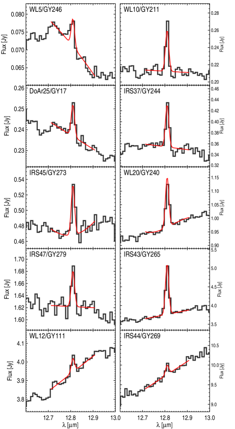
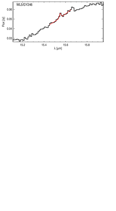
Figure 1: Spitzer/IRS spectra in the [Ne II] 12.81$\mu$m region for the ten YSOs for which the line was detected (upper panels), and in the [Ne III] 15.55$\mu$m region for the single detection of this line (lower panel). The smooth (red) lines are the sum of the continuum fits used to measure the lines and Gaussians (of fixed width and cetenred at the nominal line wavelengths) with integral equal to the line fluxes measured by summing over the line spectral bins (see text). Object names are given in each panel.

3.2.2 Extinction correction and luminosities

In order to correct the line (and continuum) fluxes for extinction we have chosen, for each of our YSO, a best-guess extinction ($A_{\rm J}$) from the up-to three estimates at our disposal. The $A_{\rm J}$ values from Tab. 2, estimated from the 2MASS photometry, were adopted when available. We otherwise estimated $A_{\rm J}$ from the $N_{\rm H}$ values given by the X-ray spectral fits (Tab. 4), converted according to Vuong et al. (2003) ($\rm A_{J}=1.8\cdot 10^{-22}$ $N_{\rm H}$). Finally, in the absence of the previous two estimates, we computed $A_{\rm J}$ from the $A_{\rm V}$ values given by the SED model fits and listed in Tab. 3: $A_{\rm J}=0.282$ $A_{\rm V}$ (Rieke & Lebofsky, 1985). We make an exception to this rule for WL12/GY111, for which the $N_{\rm H}$ value is very uncertain and we prefer to use the extinctions from the SED fit. Table 5 lists these three estimates, along with uncertainties for the latter two, and the adopted $A_{\rm J}$ value. For extinctions taken from Tab. 2 we adopted a 1 $\sigma$ uncertainty of 1 magnitude.

Critical for the derivation of unabsorbed fluxes is the choice of extinction-law, i.e., in the cases of the [Ne II] and [Ne III] lines, the two ratios $A_{12.81}/A_{J}$ and $A_{15.55}/A_{J}$. The extinction law at these wavelengths, in between two strong silicates absorption features at 9.7$\mu$m and 18$\mu$m, is not well established and seems to depend significantly on the grain characteristics (Weingartner & Draine, 2001; Draine, 2003). Chapman et al. (2009) have recently established that, for stars in the $\rho$ Ophiuchi region with low absorption ($A_{K}<0.5$), the $R_{V}=3.1$ extinction law computed by Weingartner & Draine (2001) for a “standard” grain size distribution fits the measurements between 1.25$\mu$m to 24$\mu$m. The extinction law of highly absorbed stars ($A_{K}>2$), however, is better reproduced by the $R_{V}$=5.5 Weingartner & Draine (2001) extinction law, implying grain growth in the dense parts of the cloud. Since, with one exception, the stars in our sample are highly extincted we adopt the $R_{V}$=5.5 extinction law and specifically $A_{12.81}/A_{J}=0.16$ and $A_{15.55}/A_{J}=0.13$.

With $A_{\rm J}$ ranging from 0.7 to 25 mag, the resulting correction factors for the [Ne II] 12.81$\mu$m line fluxes range from $\sim$1.1 to $\sim$39 (mean: 5.9). Note that the difference with the $R_{V}=3.1$ extinction law is significant: had we adopted it ($A_{12.81}/A_{J}=0.097$) the 12.81$\mu$m correction factor would have ranged from 1.1 to 9.5 (mean 2.7).

Table 5: Different estimates of the $J$-band extinction for the objects in our sample, and adopted value (cf. § 3.2.2).

	$A_{J}$ [mag]
Name	Lit.	$N_{H}$		SED		Adopted
DoAr25/GY17	0.7	1.7	${}_{1.6}^{1.8}$	0.5	${}_{0.2}^{0.8}$	0.7
IRS14/GY54	5.2			5.0	${}_{4.9}^{5.0}$	5.2
WL12/GY111		26.1	${}_{12.7}^{70.0}$	15.8	${}_{12.8}^{17.7}$	15.8
WL22/GY174		25.2	${}_{19.2}^{32.7}$	17.9	${}_{17.4}^{456.7}$	25.2
WL16/GY182	10.0			8.6	${}_{7.8}^{9.2}$	10.0
WL17/GY205	11.3	6.7	${}_{3.9}^{10.5}$	11.9	${}_{11.1}^{13.0}$	11.3
WL10/GY211	4.5	5.0	${}_{4.1}^{5.9}$	4.5	${}_{4.2}^{4.7}$	4.5
EL29/GY214		11.4	${}_{10.4}^{12.8}$	11.9	${}_{10.5}^{12.6}$	11.4
GY224	8.6	6.1	${}_{4.7}^{8.0}$	10.2	${}_{9.8}^{10.6}$	8.6
WL19/GY227	16.3	17.7	${}_{15.1}^{20.6}$	14.9	${}_{14.8}^{15.4}$	16.3
WL11/GY229	4.3			5.2	${}_{5.0}^{5.3}$	4.3
WL20/GY240		4.1	${}_{3.9}^{4.3}$	6.7	${}_{6.0}^{9.9}$	4.1
IRS37/GY244		10.4	${}_{7.1}^{15.7}$	11.8	${}_{10.8}^{12.7}$	10.4
WL5/GY246	16.8	11.8	${}_{10.6}^{13.0}$	14.5	${}_{12.3}^{18.3}$	16.8
IRS42/GY252	7.5	7.0	${}_{4.8}^{9.3}$	8.3	${}_{8.2}^{11.9}$	7.5
GY253	8.8	6.1	${}_{5.7}^{6.5}$	8.1	${}_{7.9}^{8.3}$	8.8
WL6/GY254	18.6	10.2	${}_{7.5}^{13.1}$	14.9	${}_{14.2}^{18.4}$	18.6
CRBR85				19.0	${}_{18.6}^{19.6}$	19.0
IRS43/GY265		8.2	${}_{7.9}^{8.5}$	13.4	${}_{12.5}^{14.4}$	8.2
IRS44/GY269		12.8	${}_{12.2}^{13.5}$	16.1	${}_{14.5}^{17.8}$	12.8
IRS45/GY273	6.6	1.8	${}_{0.6}^{3.3}$	8.3	${}_{7.7}^{8.9}$	6.6
IRS46/GY274		15.1	${}_{10.1}^{23.6}$	9.1	${}_{8.4}^{9.6}$	15.1
IRS47/GY279	7.4	3.5	${}_{2.3}^{5.2}$	8.7	${}_{8.3}^{9.4}$	7.4
GY289	7.3	3.5	${}_{3.0}^{3.9}$	6.6	${}_{6.1}^{7.0}$	7.3
GY291	7.4	4.2	${}_{3.6}^{4.7}$	6.9	${}_{6.6}^{7.2}$	7.4
IRS48/GY304				7.4	${}_{5.0}^{9.9}$	7.4
IRS51/GY315	12.9	6.2	${}_{5.5}^{6.8}$	8.6	${}_{7.6}^{9.2}$	12.9
IRS54/GY378	6.2	35.8	${}_{11.6}^{76.5}$	7.4	${}_{7.0}^{7.9}$	6.2

[Ne II] and [Ne III] line luminosities were finally derived from the measured fluxes, assuming a distance of 120 pc. Resulting line luminosities and upper limits for the whole sample are listed in Table 4, along with absorption-corrected continuum flux densities at the nominal line wavelengths. The reported uncertainties reflect measurement errors as well as uncertainties in $A_{\rm J}$, but neglect possible systematic uncertainties related to the extinction law.

We conclude this section with a cautionary note: the adopted extinction values refer to the central objects. The luminosity corrections are thus valid only if the bulk of the [Ne II] and [Ne III] lines originates in the proximity of the YSOs. This assumptions may be false for emission from shocks associated with jets and outflows.

4 Results

4.1 The [Ne II] line

We detect [Ne II] $12.8\,\mu$m line emission in 10 out of the 28 YSOs observed with Spitzer/IRS within the DROXO field of view (cf. Fig. 1). In one case, WL5/GY246, we also detect the [Ne III] $15.5\,\mu$m line. All the [Ne II] detections in $\rho$ Oph are X-ray sources: 9 are DROXO sources and the tenth, IRS37/GY244, was detected in an earlier Chandra observation (Imanishi et al., 2001, see § 3.1.2). Conversely the line is not detected in any of the three X-ray undetected objects.

We investigated possible relations between the [Ne II] line emission and other physical parameters of the systems. First, however, we discuss an important observational bias, namely the dependence of our line detection sensitivity on the continuum intensity. Figure 2 shows the relation between the [Ne II] line luminosity and the continuum flux density at the same wavelength. Both quantities are corrected for interstellar extinction and stars of different evolutionary classes are plotted with different symbols. The lower boundary of detections and upper limits clearly shows a positive correlation, most likely due to the expected anti-correlation between the detection sensitivity and the counting-statistic uncertainties (that increase with the continuum). The upper envelope however also shows a correlation, which is independent of this detection bias and whose physical origin is to be understood. Figure 2 also indicates that Class I objects have higher continuum flux densities and [Ne II] line luminosities than Class II and Class III objects. This is not immediately interpretable in terms of the X-ray excitation mechanism discussed in the introduction.

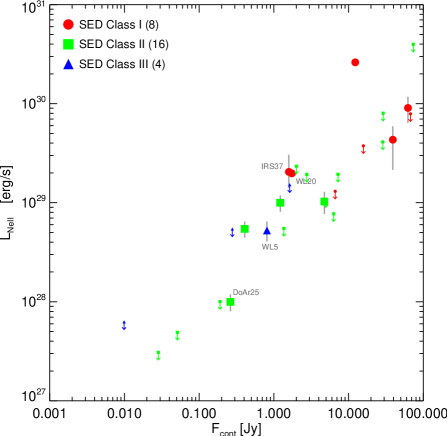
Figure 2: [Ne II] 12.81$\mu$m line luminosity vs. the continuum flux density at the same wavelength. Both quantities are corrected for interstellar extinction. Class I, Class II, and Class III objects, according to the classification derived from the SED fits, are indicated with different symbols (see legend).

Figure 3 shows the scatter plot between the [Ne II] line luminosity and $L_{\rm X}$ in the $0.3-10$ keV band. We also plot the six T-Tauri stars in the Pascucci et al. (2007) sample (four [Ne II] detections and two upper limits) and two stars (CS Cha and TW Hya) from Espaillat et al. (2007). Also shown are the theoretical predictions by MGN 08, calculated, as a function of $L_{\rm X}$, assuming the D’Alessio et al. (1999) disk model ($M_{*}=0.5M_{\odot}$, $R_{*}=2.0R_{\odot}$ , $T_{*}=4000K$, $\dot{M}=10^{-8}M_{\odot}$ yr^-1), and the predictions of GH 08 for their fiducial model (model “A”: $M_{*}=1.0M_{\odot}$, $R_{*}=2.61R_{\odot}$ , $T_{*}=4278K$, $\dot{M}=3\cdot 10^{-8}M_{\odot}$ yr^-1, $L_{\rm FUV}=10^{31.7}$ erg/s) and two variations: model “B” (with 100 times lower dust opacity, taken to represent an evolved disk) and model “D” (with 10 times higher FUV flux).

Three conclusions are apparent: i) no overall trend of increasing [Ne II] line luminosity with $L_{\rm X}$ is apparent; ii) two of the 10 measured [Ne II] luminosities, those of DoAr 25 and WL 5/GY 246, as well as the 18 upper limits, are consistent with predictions by current models for X-ray ionization of the disk; iii) the remaining 8 measured [Ne II] luminosities are 1 to 3 orders of magnitude brighter than predicted. With respect to this latter point it is important to note, however, that the authors of both calculations stress that their models refer to objects with specific star and disk parameters and are moreover affected by several uncertainties, e.g. in the atomic physics, in the simplified disk models that do not include holes, gaps, and rims, and in the current lack of EUV photoexcitation. Our findings indeed confirm these suspicions, and indicate that physical parameters other than $L_{\rm X}$ are likely to be important in determining the [Ne II] line luminosity.

Rather than a connection with $L_{\rm X}$, Fig. 3 indeed suggests that the [Ne II] flux might be related to the evolutionary state of the YSOs, Class I being the strongest and Class III the faintest emitters. The position of TW Hya and of the six Pascucci et al. (2007) ‘transition disk’-systems, seems consistent with this interpretation. CS Cha, also believed to host a transition disk has hower a strong [Ne II] emission in line with that of most of the [Ne II] detections in our sample. Within our sample, the higher [Ne II] luminosity of Class I objects with respect to Class II ones is confirmed with significances ranging from 99.8% to 99.99% by the five two-population tests for censored data implemented in the ASURV package (Feigelson & Nelson, 1985; Isobe & Feigelson, 1990).

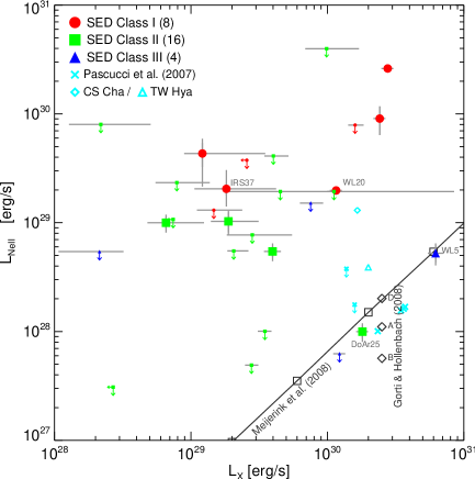
Figure 3: [Ne II] luminosity vs. $L_{\rm X}$. Symbols as in Fig. 2. The 1 $\sigma$ error bars for the [Ne II] luminosity account for uncertainties in the measurement errors and in the extinction correction. For the X-ray luminosities estimated from DROXO data errors come from the statistical uncertainty of the normalization of the best-fit emission models, while for the Chandra ACIS detections we assumed a 50% uncertainty. Also plotted here are the six T-Tauri stars in the Pascucci et al. (2007) sample and two stars from Espaillat et al. (2007) (CS Cha and TW Hya). The model predictions of MGN 08 are indicated by the diagonal line; those of GH 08, for their models ‘A’, ‘B’, and ‘D’ by the three diamond symbols.

The overall lack of correlation with X-ray luminosity leads us to investigate possible correlations of the [Ne II] emission with other stellar and circumstellar parameters. Figure 4 shows the relations with disk mass accretion rate and with stellar mass, both estimated from the SED fits. Also shown are the MGN 08 and the GH 08 model predictions. The most fundamental of stellar parameters, mass, does not seem to influence the [Ne II] luminosity. At any given mass, Class I objects have significantly higher line luminosities with respect to Class II and Class III ones; this points toward a role of parameters related to the YSO evolution, such as matter inflows and outflows. The [Ne II] luminosity seems indeed to to correlate with $\dot{M}$. Statistical tests for censored data, the Generalized Kendall’s $\tau$ and the Spearman’s $\rho$ as implemented in the ASURV package, confirm the existence of a correlation with $\sim$99.5% confidence. The stars from Pascucci et al. (2007) and Espaillat et al. (2007), shown in Fig. 4 but not used for the correlation tests, appear compatible with our sample. The correlation with $\dot{M}$ may also explain the correlation of the [Ne II] luminosity with the continuum flux at 12.81 $\mu$m (Fig. 2) as this latter correlates strongly with $\dot{M}$ (not shown, confidence $\sim$99.99%). The [Ne II] - $\dot{M}$ correlation might also explain, at least in part, the difference in the [Ne II] luminosity among the different evolutionary classes as Class I objects have statistically higher accretion rates.

As for the discrepancy with the X-ray excitation models, we note that three out of five Class I [Ne II] detections have nominal accretion rates that are higher than those used as inputs for both of the models considered here. This might be the reason for their higher than predicted line luminosities. The other Class I [Ne II] detections, WL 20 and IRS 37, however, have $\dot{M}$ estimates that, although with large uncertainties, are similar to those assumed by the X-ray ionization models and still their line luminosity is much larger than predicted. It is also possible that the [Ne II]-$\dot{M}$ correlation simply results from Class I objects having brighter line emission due to a mechanism unrelated to disk mass accretion. One good candidate might be the defining characteristics of Class I objects, i.e. high envelope accretion rates and/or their associated outflows. Indeed the [Ne II] luminosity also shows a significant correlation, at the $\sim$99.9% level, with the $\dot{M}_{\rm env}$ values derived from the SED fits.

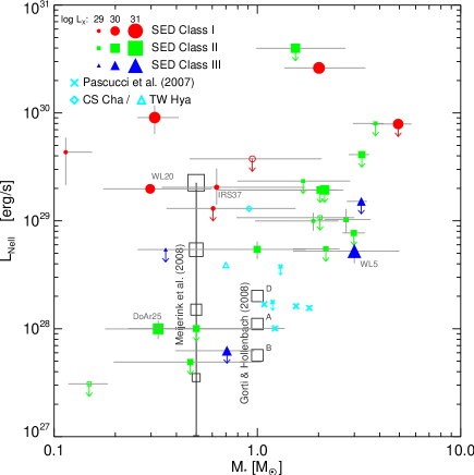
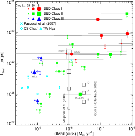
Figure 4: [Ne II] luminosity vs. $M_{*}$ (left panel) and $\dot{M}_{\rm disk}$ (right panel). Symbols as in Fig. 2 and 3, but with size proportional to $\log L_{\rm X}$, as exemplified in the legend. The three X-ray undetected objects are indicated by empty symbols. Model results are plotted as in Fig. 3.

4.2 The [Ne III] line

A spectral feature at $\sim 15.55$ $\mu$m, likely associated with a [Ne III] transition, is detected in only one star, WL 5. An alternative identification for the observed feature might be a water rotational transition at 15.57 $\mu$m, as detected e.g. by Carr & Najita (2008) and Salyk et al. (2008) in three CTTs. The line observed on WL 5 is however well centered at 15.55 $\mu$m (cf. Fig. 1) and the wavelength difference with the water line is significant: $\sim$2 spectral bins or about the FWHM spectral resolution. Moreover the many other water lines that are seen in the spectra published by Carr & Najita (2008) and Salyk et al. (2008) are not visible in the part of the WL 5 spectrum shown in Fig. 1, with the exception of a likely H₂O line at 15.67 $\mu$m. We are therefore confident in the identification of the line with [Ne III].

WL 5 is a Class III object and, according to its F7 spectral type (Greene & Meyer, 1995), one of the most massive/hottest objects of the sample of [Ne II] detections (see the Appendix for a detailed discussion of its properties). For both Neon lines, WL 5 has the lowest observed (i.e. absorbed) continuum flux among the stars in which [Ne II] was detected, thus facilitating the detections of the lines. The luminosities of both Neon lines compare reasonably well with the prediction of MGN 08 for the $L_{\rm X}$ of the object (6.2$\times$10³⁰ erg $s^{-1}$): the [Ne II] line is only 7% fainter than predicted (well within 1$\sigma$) and the [Ne III] line is 70% brighter than predicted (within 2$\sigma$).

All the other stars with [Ne II] detection in our sample have [Ne III] upper limits that are significantly larger and therefore compatible with the predictions of MGN 08. If we assume that the line ratios predicted by MGN 08, rather than the luminosities, are correct and use the measured [Ne II] line luminosities to predict [Ne III] luminosities, we conclude that, for 8 out of 9 stars, our detection sensitivity for [Ne III] is too low by a factor 2.4-8. For the remaining case, IRS 43/GY 265, the star in our sample with the brightest [Ne II] line, the measured upper limit is only 10% higher than the predicted [Ne III] flux.

5 Summary and discussion

We investigated the origin of the [Ne II] and [Ne III] fine structure lines by studying a sample of 28 $\rho$ Ophiuchi members in the field of view of the DROXO deep X-ray observation and with available Spitzer IRS data. The [Ne II] 12.81 $\mu$m and the [Ne III] 15.55 $\mu$m lines were detected in ten and one YSOs, respectively; absorption corrected line luminosities and upper limits for non-detections were computed and compared with predictions of X-ray disk ionization models. Finally, we explored empirical relations between [Ne II] line luminosity and stellar and circumstellar parameters estimated by fitting the SEDs of the objects with star/disk/envelope models.

The luminosities of the 10 detected [Ne II] lines are, for the most part, 1-3 dex higher than predicted by models of X-ray irradiated (and ionized) circumstellar disks. Moreover, the [Ne II] luminosities do not correlate with the X-ray luminosities. We conclude that, if these lines are indeed produced by X-ray ionization, factors other than $L_{\rm X}$ are also important for the line production. Published models might still be valid: since they assume given star and disk characteristics (or few variations) it is possible that some of these assumptions are critical and that they do not correspond to the characteristics of most of our stars. Other excitation mechanisms might, however, turn out to be more important than X-rays, such as strong shocks resulting from the interaction of the stellar wind and jets with circumstellar material (Hartmann & Raymond, 1989; Hollenbach & McKee, 1989; van Boekel et al., 2009).

Interestingly, the [Ne II] luminosities of two of the objects in our sample, DoAr 25 and WL 5/GY 246, match the theoretical prediction for X-ray irradiated disks remarkably well. DoAr 25 is a Class II object with mass accretion rate similar to that assumed by the models we have used for comparison. WL 5 is, based on its SED between 1 and 8 $\mu$m, a Class III object, but we cannot exclude the presence of a gas disk or a dust disk with a large inner hole. It might be similar to the four stars with transitional disks studied by Brown et al. (2007), for one of which, T Cha, the [Ne II] line was detected by Lahuis et al. (2007). WL 5 is, moreover, together with Sz 102 (Lahuis et al., 2007), the second YSO for which a detection of the [Ne III] line has been reported. As for the [Ne II] line, the luminosity of the [Ne III] line of WL 5 is roughly consistent with theoretical predictions for the X-ray irradiation mechanism. Also largely consistent with this mechanism are the upper limits to the luminosities of the undetected [Ne II] and [Ne III] lines.

The [Ne II] 12.81 $\mu$m line luminosity correlates with the continuum flux at the same wavelength. While the lower envelope of the relation may be explained with a sensitivity bias, the upper envelope likely reflects a correlation with some physical characteristics to which the continuum flux is related. Disk accretion rate, which we have found to correlate with the continuum flux at 12.81 $\mu$m, is one candidate, and indeed the [Ne II] luminosity correlates with it. A tentative physical explanation of the correlation might involve the increased EUV flux produced in the accretion shock, provided that this latter is able to reach and significantly ionize neon atoms above the accretion disk. Alternatively, given the correlation generally found between accretion and outflow rates, the correlation might result from the [Ne II] emission being produced in outflow-related shocks as mentioned above. Finally, the statistical correlation might be unphysical, and simply driven by the higher accretion rates of Class I objects combined with their higher [Ne II] luminosities.

Indeed, Class I objects, i.e. those with significant envelope accretion, have significantly higher [Ne II] luminosities than Class II objects. We propose that the presence of a circumstellar envelope and/or envelope accretion and/or the strong associated outflows, i.e. the defining characteristics of Class I objects, plays a role in determining the line emission. Larger YSO samples and more sophisticated theoretical models are needed to pinpoint the production mechanism of these gas-tracing lines and to derive a consistent picture of the environment around YSOs at different evolutionary stages.

Appendix A (Circum)Stellar parameters from SED fits

In this appendix we describe how we constrained some stellar and circumstellar parameters of the objects in our sample by comparing their SEDs with the theoretical models of Robitaille et al. (2006). These consist of a grid of 200,000 model SEDs that include contributions from the central star, the circumstellar disk, and the envelope, parametrized with 14 parameters. The models that best approximate the observed SEDs were found with the aid of the Web based tool presented by Robitaille et al. (2007). As stated by Robitaille et al. (2007), and in accord with basic principles, this method does not allow the simultaneous determination of all the 14 physical parameters, since the SEDs are often defined by less than 14 independent fluxes. However, depending on the available fluxes, some of the parameters can be constrained more narrowly than others. We are here interested, in particular, in obtaining the range of values compatible with the observed SEDs for: $i$) the extinction toward our objects, $ii$) their disk accretion rates.

A.1 The method and its validation

Our procedure follows closely that of Robitaille et al. (2007): from the Web interface we obtain, for each object, a list of the 1000 models that best approximate the observed SEDs, i.e. those with the smallest $\chi^{2}$. Our “best guess” parameter values and associated confidence intervals are then derived by selecting a set of statistically reasonable models and computing the median and the $\pm 1\sigma$ quantiles of the parameter values for these models. The statistically reasonable models were defined as those with reduced $\chi^{2}<(\chi^{2}_{\rm best}+3)$, where $\chi^{2}_{\rm best}$ refers to the best fit model, or in cases this condition results in less than 10 models, the 10 models with smallest $\chi^{2}$. Note that, because the uncertainties on the observed SEDs are not well defined (see below), and the parameter space is sampled only discretely by the adopted grid of models, the statistical significance of the thus derived confidence intervals cannot be easily assessed.

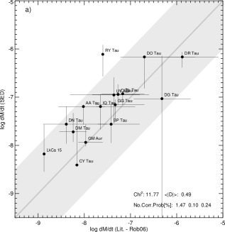
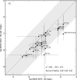
Figure 5: Comparison between mass accretion rates from the literature and those derived from SED fits for the sample of T-Tauri stars considered in Robitaille et al. (2006). SED fits and determination of parameter ranges were performed as for the $\rho$ Ophiuchi objects discussed in this paper. Panel $a)$ compares the literature data with results of SED fits using all the available photometry, including optical bands. Panel $b)$ is analogous, but only photometry longward of 1$\mu$m was used for the SED fits. Panel $c)$ finally compares the results of SED fits with and without optical photometry. Reduced $\chi^{2}$ values and mean absolute distances from the bisector, both computed considering uncertainties on the abscissa only, are reported within each panel.

A similar method was tested by Robitaille et al. (2007) by considering a sample of Taurus-Auriga objects for which stellar and circumstellar parameters had been derived independently in the literature and comparing these parameters with those obtained from fitting the SEDs, defined from the optical to millimeter wavelengths. In the case of our heavily absorbed $\rho$ Ophiuchi YSOs the SEDs lack, with the exception of one star, data in the optical bands, i.e. those more directly affected by the accretion-shock emission. In order to test our ability to constrain the accretion rates in the absence of optical information, we repeated the SED fits of the Taurus-Auriga stars of Robitaille et al. (2007), using the same datapoints to define the SEDs, and both including and excluding the optical magnitudes. The results are shown in Fig. 5. Panel $a)$, analogous to Fig 2b in Robitaille et al. (2007), compares the accretion rates derived from the SED fits, including optical data, with independent values from the literature. Panel $b)$ compares the results of the SED fits without the optical magnitudes with the literature data. The agreement between the two quantities is acceptable and may actually be considered better than in the former panel: the reduced $\chi^{2}$, computed from the identity relation considering only uncertainties on $\dot{M}_{SED}$, is indeed reduced from $\sim$12 to 1.7. This can in part be attributed to the increased error bars; note, however, that the average of the unsigned differences, abs($\dot{M}_{SED}$-$\dot{M}_{Lit.}$), is almost unchanged, 0.49 dex for panel $a)$ and 0.48 dex for panel $b)$. Panel $c)$ compares the $\dot{M}$ from the SED fits with and without optical magnitudes, showing that the two sets of values agree within uncertainties. We conclude that the SEDs defined from IR to millimeter wavelengths are indeed sensitive to the accretion rate, at least in the $\dot{M}$ range covered by the Taurus-Auriga sample: log $\dot{M}$=[-8.5,-6].

This is due to the effect of viscous heating affecting the disk thermal structure. To exemplify this effect we plot in Fig. 6, as a function of accretion rate, the ratio between the IRAC 3 band and the $J$-band flux, for the Robitaille et al. (2006) models for stars with mass between 0.7 and 1.3 M_⊙, age between 1 and 2 Myr (implying little or no circumstellar envelope), and low disk inclination with respect to the line of sight ($i<$60^∘). We plot with different symbols models with disk inner radii in different ranges, since the inner hole affects the flux at the IRAC 3 wavelength (5.8 $\mu$m). A relation between the two quantities is seen for models with moderate inner disk holes, apparently characterized by different regimes in three different $\dot{M}$ ranges: $\log(\dot{M}/M_{\odot})\lesssim-11$, $-11\lesssim\log(\dot{M}/M_{\odot})\lesssim-9$, and $\log(\dot{M}/M_{\odot})\gtrsim-9$. The factor of $\sim$2 scatter around this relation may likely be attributed to model variations within the specified parameter ranges and to the several other unconstrained model parameters. Similar and even more pronounced trends are apparent in analogous plots using fluxes in longer wavelength IRAC and MIPS bands, with the expected difference that at the longer wavelengths, emitted farther out in the disk, the size of the inner hole has a much smaller effect. The three regimes in Fig. 6 can be understood as follows: $i$) for large accretion rates, $\log(\dot{M}/M_{\odot})\gtrsim-9$, the flux in the IRAC band, originated in the inner disk (R$<$1 AU), is significantly affected by viscous accretion (D’Alessio et al. 1998, 1999); $ii$) for $-11\lesssim\log(\dot{M}/M_{\odot})\lesssim-9$ disk heating is dominated by the stellar photospheric emission and, consequently, no relation between the IRAC flux and $\dot{M}$ is observed; $iii$) for $\log(\dot{M}/M_{\odot})\lesssim-11$ we again observe a direct relation between the IRAC 3 flux and $\dot{M}$, which we attribute to the fact that these low accretion rates correspond, in the Robitaille et al. (2006) model grid, to very low disk masses (M${}_{\rm disk}\lesssim 10^{-6}$M _⊙ for the $\sim$1 solar mass stars plotted in Fig. 6). Since, in the model grid, disk mass and accretion are directly correlated and such low mass disks are optically thin (Robitaille et al. 2006), lower accretion rates imply lower disk mass and lower emission in the IRAC band. The IRAC 3 flux vs. $\dot{M}$ correlation in this regime does not therefore imply that that the mid-IR SED carries direct information on disk accretion.

As a result of this discussion, in the derivation of accretion rates for our $\rho$ Ophiuchi sample from the SED fits, we decided not to use values below $10^{-9}$M _⊙ yr^-1. In such cases we instead conservatively assigned upper limits to $\dot{M}$ equal to the maximum between $10^{-9}$M _⊙ yr^-1 and the upper end of the $\dot{M}$ confidence interval (see above).

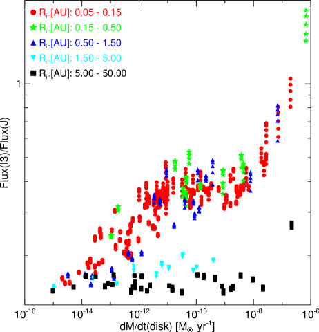
Figure 6: Scatter plot of the ratio between the flux in the IRAC 1 band over that in $J$, as a function of disk accretion rate, according to the Robitaille et al. (2006) models for a solar mass stars. Each point corresponds to one of the Robitaille et al. (2006) models satisfying the following conditions: mass of the central object between 0.7 and 1.3 M_⊙, age between 1 and 2 Myr, and disk inclination with respect to the line of sight $<$60^∘. Different symbols indicate models with inner disk radius in five ranges as indicated in the legend.

A.2 The $\rho$ Ophiuchi sample

We collected photometric measurements and uncertainties (when available) for our $\rho$ Ophiuchi sample from several sources: $J$, $H$, and $K_{s}$ magnitudes (or upper limits) were taken for almost all objects from 2 MASS; Spitzer IRAC (bands 1-4) and MIPS (bands 1 & 2) photometry was collected from the c2d database (Evans et al. 2003); 1.2 mm fluxes were collected from Stanke et al. (2006) and 1.3 mm fluxes from Andre & Montmerle (1994). Optical $UBVR$ photometry for one object with small absorption (DoAr 25) was taken from Yakubov (1992). Table 6 list all the photometric flux densities collected from the literature.

Finally we complement the photometric data with flux densities from the IRS spectra (cf. § 2.1). We computed flux densities between 10 and 18$\mu$m, at regular wavelength intervals spaced by 0.5$\mu$m. Each flux density was taken as the average of the spectral bins in 0.2$\mu$m intervals centered at the nominal wavelength. For the four stars with two IRS observations we have taken the average of the two spectra. (In three cases the wavelength-averaged fluxes differ by less than 0.1 dex, while in one case, EL29/GY214, the difference is 0.4 dex. In all cases we verified that the results of the model fits did not change appreciably choosing either of the two spectra). Table 7 lists the flux densities from the IRS spectra. As stated in § 2.1 our sky subtraction procedure does not take into account diffuse nebular emission. In order to assess the significance of diffuse emission on the object flux densities, we have considered the IRS spectra of the 13 YSOs in our sample observed in the context of the Spitzer legacy program From Molecular Cores to Planet-Forming Disks (‘c2d’, Evans et al. 2003). As with the entire c2d sample, the reduced/sky-subtracted IRS spectra have been analyzed (and made publicly available) by the c2d team, using a sophisticated extraction and sky subtraction method based on the modelling of the cross dispersion profiles (Lahuis et al. 2007). We have compared the flux densities derived from the c2d-reduced spectra with those derived from the same spectra reduced by us. We find the spectra to be similar, with both the maximum and the wavelength-averaged discrepancy decreasing with object intensity. The maximum discrepancy falls below 10% for the 9 YSOs with c2d-reduced spectra that have average flux $>$0.5 Jy. Based on this comparison, and noting that the c2d objects are representative of our sample as for their position with respect to nebulosity seen in IRAC and MIPS maps, we decided to use the IRS-derived fluxes for defining the SEDs of the 17 stars with average IRS flux $>$0.5 Jy.

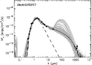
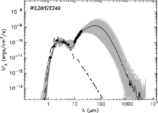
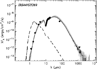
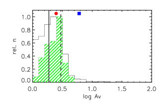
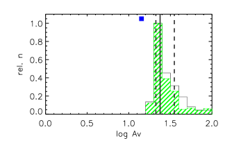
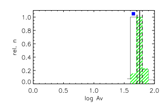
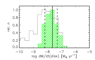
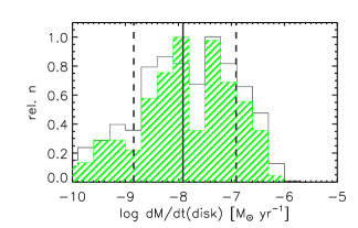
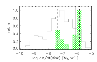
Figure 7: Examples of SED fits for three objects in our sample with [Ne II] detections. From left to right: DoAr25/GY17, WL20/GY240, and IRS44/GY269. The first is classified as Stage/Class II, the other two as Stage/Class I. The upper row shows the SEDs and the best fit models as produced by the Web interface provided by Robitaille et al. (2006). For the datapoints, detections and upper limits are indicated by circles and triangles, respectively. The lower two rows represent distributions of two fit parameters, $A_{\rm V}$ and $\dot{M}_{\rm disk}$. The empty histograms refer to the 1000 model fits with lowest $\chi^{2}$ and the green histograms to the statistically reasonable samples of models defined in § A.1. The solid and dashed vertical lines indicate the median and the 1$\sigma$ dispersion for these latter samples. For the panels in the second row the symbols close to the upper axis indicate the $A_{\rm V}$ values inferred from the $A_{\rm J}$ in Table 2 (circles) and from the X-ray derived $N_{\rm H}$ in Table 4 (squares).

As suggested by Robitaille et al. (2007), in order to account for systematic uncertainties, underestimation of the measurement errors, and intrinsic object variability in time, a lower limit of 25%, 10%, and 40% was imposed on the uncertainties of optical, NIR/MIR, and millimeter fluxes, respectively.

Figure 7 exemplifies the “fitting” procedure described in § A.1 for three of our YSOs. It shows the SEDs with the best fit models and the distributions of two fit parameters, $A_{\rm V}$ and $\dot{M}_{\rm disk}$, both for the 1000 models with lowest $\chi^{2}$ and for the statistically reasonable ones (cf. A.1). SEDs and best fit models for all the 28 YSOs in our sample are shown in Fig. 8.

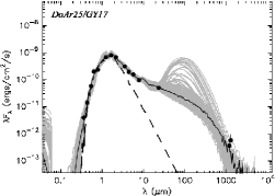
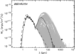
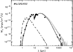
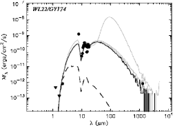
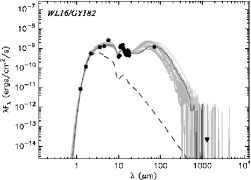
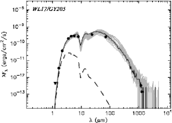
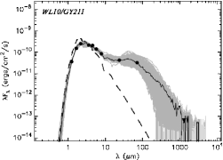
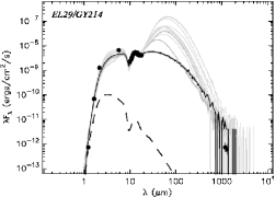
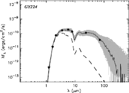
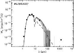
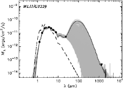
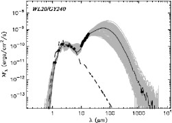
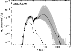
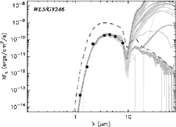
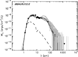
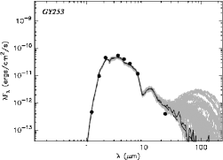
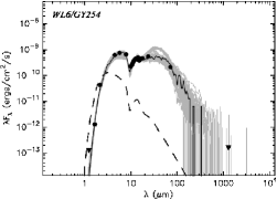
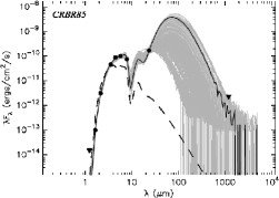
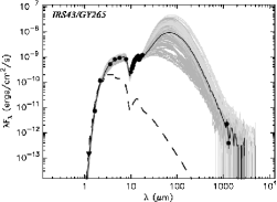
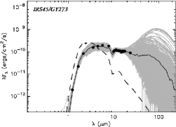
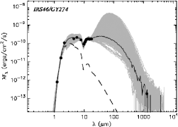
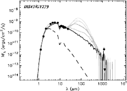
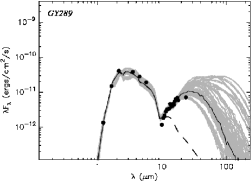
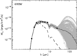
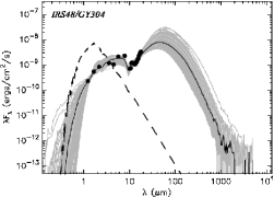
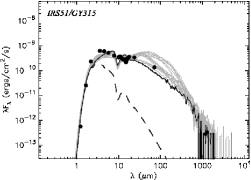
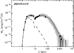
Figure 8: SEDs and best fit models, as produced by the Web interface provided by Robitaille et al. (2006), for all the 28 YSOs in our sample.

Following visual examination of the SED fits and of the distributions of model parameters used to define the confidence intervals, we have decided to modify the input datapoints for two objects: for IRS45/GY273 we have excluded the 1.2 and 1.3 mm datapoints from Stanke et al. (2006) and Andre & Montmerle (1994); in both cases including these points significantly worsened the quality of the fit and had a significant effect on the values of the parameters. The 1.2 mm flux is $>$20 times higher than the 1.3 mm flux (an upper limit) and probably refers to an extended source that includes our YSO. For GY289, a source with average IRS flux $<$0.5 Jy, we have decided to include the IRS datapoints because: $i)$ they agree quite well with the MIPS fluxes at similar wavelengths, $ii)$ the quality of the model fit is reasonable ($\chi^{2}_{\rm best}\sim$2) and, $iii)$ the confidence intervals of the model parameters are narrower but compatible with those from the fit performed without these points.

Finally for one object, WL5/GY246, we could not obtain a unique fit with the above procedure. The object was previously classified as a deeply absorbed Class III star with an F7 spectral type (Greene & Meyer 1995), and our SED was defined by $J$,$H$,$K$, Spitzer IRAC 1-4 and 1.2/1.3mm fluxes. Fits both with and without the mm fluxes, likely contaminated by nearby sources (c.f. Andre & Montmerle 1994; Stanke et al. 2006), consistently yield high envelope and/or disk accretion rates, typical of a Class I object, but having little effect on the NIR/MIR part of the SED due to the associated large inner disk radii. The NIR/MIR SED can however be fit equally well by purely photospheric ‘Phoenix’ models as suggested by the same Robitaille et al. (2007) web interface used to fit the star/disk/envelope models. We thus decided to assume that WL5/GY246 is a Class III object and to derive its extinction, effective temperature, and stellar mass using the $J$, $H$, and $K$ photometry, the spectral type, and the calibrations tabulated by Kenyon & Hartmann (1995). Uncertainties were estimated from the assumed uncertainty on the spectral type, one subclass, and the range of values obtained by estimating the absorption from the J-H, H-K, and J-K colors.

Table 3, introduced in the main text (§2.3) lists the outcome of the SED-fit process: the quality of the fit (the $\chi^{2}$ of the “best-fit” model), the object extinction (the sum of interstellar and envelope extinction), the stellar effective temperature and mass, the disk mass, the disk and envelope accretion rates, the evolutionary Stage. This latter quantity was assigned following Robitaille et al. (2007). Stage I: $\dot{M}_{\rm env}/M_{*}>10^{-6}$; Stage II: $\dot{M}_{\rm env}/M_{*}\leq 10^{-6}$ and $M_{\rm disk}/M_{*}>10^{-6}$; Stage III: $\dot{M}_{\rm env}/M_{*}\leq 10^{-6}$ and $M_{\rm disk}/M_{*}\leq 10^{-6}$. As indicated in the main text, in order to use a more familiar designation to researchers in the field, we also refer to the ‘Stages’ as ‘Classes’.

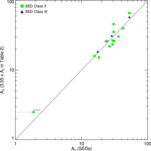
Figure 9: Comparison of the $A_{\rm V}$ values derived from fitting the SEDs with the Robitaille et al. (2006) models, with values derived from 2MASS photometry (cf. Table 2). Objects of different SED Class are indicated by different symbols as shown in the legend.

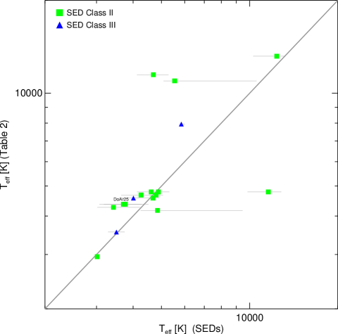
Figure 10: Same as Fig. 9 for the effective temperatures.

Figures 9 and 10 compare the extinction values ($A_{\rm V}$) and stellar $T_{\rm eff}$ obtained from the SED fits with the same parameters listed in Table 2 for Class II and Class III stars. Given the considerable uncertainties of both determinations, the SED fits yield results similar to those obtained with the method of Natta et al. (2006). A similar comparison with the accretion rates derived from the Pa$\beta$ and Br$\gamma$ NIR line fluxes (in Table  2), is less conclusive due to the large number of upper limits and to the large uncertainties that affect the spectroscopic measurements as well as the SED fits. Seven objects can be used for the comparison having accretion rate estimates or upper limits from both methods. For only two stars both methods yield estimates: those for IRS 54 are in good agreement; for WL 16 the spectroscopic estimate is 2.6 dex higher than the value from the SED fits, $\dot{M}\sim 10^{-8}$ M_⊙yr^-1. The discrepancy is however reduced to 1.2 dex when comparing the result of the SED fit with the Natta et al. (2006) value. Moreover the derivation of $\dot{M}$ from the Pa_β line with the method of Natta et al. (2006, see also §2.3) is better suited for cool stars and likely to yield inaccurate results for WL 16 ($T_{\rm eff}\sim 10^{4}$ K). An independent estimate by Najita et al. (1996) yielded an upper limit compatible with the SED value: $\dot{M}\lesssim 2\times 10^{-7}$ M_⊙yr^-1. Other three stars have $\dot{M}$ estimates from the SED fits and upper limits from Table 2: in two cases, IRS 51 and IRS 47, the confidence intervals from the SED fits are consistent with the upper limits; for DoAr 25/GY17, the only star with optical magnitudes, the SED fit yields an accretion rate that is 1.6 dex higher than the upper limit from the Pa_β line. Finally, for two stars, WL 10 and WL 11, the spectroscopic estimates are 0.4 dex and 0.1 dex larger than the upper limits from the SED fits. The discrepancy is however reduced to 0.24 dex for WL 10 and disappears for WL 11 if the slightly larger $\dot{M}$ values from Natta et al. (2006) are considered instead of those in Table 2.

A.3 Summary

In this Appendix we have shown that the SED models of Robitaille et al. (2006), although undeniably approximate, can be useful to constrain parameters such as the line-of-sight absorption and the disk accretion rate, even in the absence of optical photometry. Although resulting uncertainties in these parameters are often large, the constraints are by and large compatible with independent determinations obtained with more direct methods.

Table 6: Flux densities, in mJy, collected from the literature (cf. §A.2) and used for the SED fits.

Name	J	H	Ks	IRAC [1]	IRAC [2]	IRAC [3]	IRAC [4]	MIPS [1]	MIPS [2]	1.2mm	1.3mm
DoAr25/GY17	279.00	448.00	484.00	367.00	292.00	299.00	258.00	399.00		153.00	280.00
IRS14/GY54	1.66	12.10	30.20	35.10	29.20	23.40	14.00				$<$ 30.00
WL12/GY111	0.32	3.21	15.20	239.00	744.00	1610.00	2240.00		8120.00	415.00	130.00
WL22/GY174	$<$ 0.20	$<$ 0.08	0.59				3230.00				400.00
WL16/GY182	3.44	65.90	397.00	1400.00	1970.00	5030.00			29100.00		$<$ 10.00
WL17/GY205	$<$ 0.19	1.96	27.30	240.00	416.00	553.00	695.00	2790.00	6070.00	144.00	70.00
WL10/GY211	15.30	86.10	181.00	259.00	310.00	272.00	222.00	339.00	784.00		$<$ 30.00
EL29/GY214	0.31	39.00	929.00			12800.00				316.00	300.00
GY224	$<$ 0.20	7.21	55.70	203.00		358.00	367.00	907.00	908.00
WL19/GY227	$<$ 0.06	0.97	25.20	215.00		406.00	328.00	223.00			$<$ 20.00
WL11/GY229	0.90	5.83	17.00	33.70	35.80	34.20	31.00	43.00			$<$ 20.00
WL20/GY240	4.41	32.00	97.30	127.00	143.00	140.00					90.00
IRS37/GY244	$<$ 0.21	1.75	15.50	127.00	206.00	286.00	268.00	780.00			300.00
WL5/GY246	0.02	1.37	39.90	209.00	297.00	298.00	163.00			$<$ 375.00	35.00
IRS42/GY252	1.31	32.50	270.00	1060.00	1630.00	2100.00	2980.00	3450.00	2940.00		$<$ 35.00
GY253	0.20	5.39	32.70	64.70	60.40	53.30	30.90	3.18
WL6/GY254	$<$ 0.06	0.72	31.10		925.00	1440.00	1730.00	4360.00	5110.00		$<$ 75.00
CRBR85	$<$ 0.01	0.06	2.26	54.00	131.00	191.00	198.00	1340.00		$<$ 921.00
IRS43/GY265	$<$ 0.06	4.01	84.30	629.00	1240.00	1790.00	2190.00			967.00	190.00
IRS44/GY269	$<$ 0.38	3.46	47.00	731.00	1830.00				34700.00	$<$ 576.00	180.00
IRS45/GY273	0.81	12.20	60.70	187.00	272.00	382.00	481.00	712.00		1058.00	$<$ 40.00
IRS46/GY274	0.33	9.03	77.50		271.00	402.00	411.00				90.00
IRS47/GY279	1.19	25.40	164.00	740.00	1190.00	1580.00	2040.00	1720.00		1336.00	$<$ 20.00
GY289	0.56	8.24	29.10	45.60	41.90	36.80		56.50
GY291	0.53	8.18	27.50	54.20	69.50	84.80	108.00	94.50
IRS48/GY304	94.60	305.00	618.00	1410.00	1600.00	4060.00	6000.00				240.00
IRS51/GY315	0.24	14.40	169.00	752.00	916.00	1000.00	1070.00	2730.00	3260.00	124.00	165.00
IRS54/GY378	2.14	34.30	218.00		712.00	931.00	1010.00	3560.00	6500.00	340.00	$<$ 120.00

Note: Values in italic were not used for the SED fits.

Table 7: Flux densities, in Jy, obtained from the IRS spectra for the SED fits.

Name / $\lambda$[$\mu$m]	10.0	10.5	11.0	11.5	12.0	12.5	13.0	13.5	14.0	14.5	15.0	15.5	16.0	16.5	17.0	17.5	18.0
DoAr25	0.23	0.23	0.24	0.27	0.25	0.25	0.23	0.23	0.24	0.22	0.24	0.25	0.28	0.30	0.33	0.36	0.37
IRS14	0.022	0.022	0.040	0.094	0.096	0.11	0.098	0.081	0.066	0.061	0.062	0.066	0.073	0.11	0.11	0.095	0.067
WL12	0.93	1.3	1.7	2.3	3.0	3.7	4.1	4.3	4.5	4.7	4.1	4.1	4.4	4.2	4.3	4.4	4.5
WL22	0.16	0.25	0.62	0.87	1.0	1.4	1.1	1.1	0.96	0.96	0.44	0.48	0.96	1.5	1.3	1.4	1.1
WL16	1.3	1.5	4.4	5.1	4.8	6.3	4.4	3.8	3.2	2.9	2.6	2.4	2.9	4.4	4.0	3.9	2.7
WL17	0.18	0.21	0.27	0.31	0.34	0.37	0.42	0.48	0.48	0.52	0.51	0.54	0.64	0.64	0.70	0.74	0.76
WL10	0.17	0.18	0.19	0.20	0.21	0.21	0.21	0.22	0.22	0.22	0.23	0.24	0.25	0.26	0.27	0.27	0.28
EL29	7.2	9.5	12.	16.	19.	22.	23.	24.	24.	26.	22.	22.	24.	24.	24.	25.	25.
GY224	0.27	0.30	0.34	0.37	0.38	0.39	0.40	0.43	0.45	0.47	0.48	0.48	0.53	0.56	0.60	0.62	0.63
WL19	0.053	0.071	0.077	0.096	0.13	0.15	0.15	0.16	0.17	0.18	0.16	0.15	0.16	0.14	0.14	0.15	0.14
WL11	0.012	0.014	0.011	0.010	0.014	0.014	0.015	0.019	0.017	0.017	0.022	0.021	0.027	0.029	0.034	0.037	0.033
WL20	0.34	0.45	0.59	0.73	0.83	0.89	1.0	1.2	1.4	1.6	1.6	1.8	2.3	2.5	2.8	3.1	3.4
IRS37	0.13	0.17	0.22	0.26	0.29	0.33	0.35	0.37	0.39	0.43	0.40	0.42	0.49	0.53	0.57	0.63	0.66
WL5	0.015	0.021	0.029	0.037	0.052	0.064	0.062	0.066	0.065	0.066	0.047	0.047	0.068	0.079	0.088	0.11	0.098
IRS42	1.8	2.0	2.3	2.4	2.1	2.1	2.1	2.1	2.1	2.2	2.1	2.1	2.4	2.4	2.4	2.6	2.7
GY253	9.4e-05	0.00031	-0.0015	-0.0021	0.0024	0.00084	0.0028	0.0059	0.0035	0.0023	0.0051	0.0024	0.0047	0.0048	0.0080	0.0092	0.0058
WL6	0.73	0.92	1.1	1.4	1.6	1.8	2.0	2.1	2.2	2.4	1.9	2.0	2.4	2.5	2.6	2.7	2.8
CRBR85	0.066	0.10	0.14	0.18	0.23	0.27	0.31	0.35	0.39	0.43	0.35	0.37	0.49	0.51	0.55	0.62	0.65
IRS43	0.87	1.2	1.7	2.3	2.9	3.5	4.0	4.4	4.9	5.4	4.0	4.4	5.6	5.8	6.3	6.8	7.3
IRS44	1.5	2.4	3.5	5.3	7.2	8.7	10.	12.	13.	15.	13.	14.	17.	18.	20.	22.	24.
IRS45	0.34	0.40	0.44	0.48	0.46	0.48	0.48	0.50	0.52	0.53	0.49	0.52	0.59	0.57	0.60	0.64	0.63
IRS46	0.31	0.39	0.48	0.57	0.66	0.72	0.76	0.81	0.83	0.87	0.85	0.88	0.93	0.96	1.0	1.0	1.1
IRS47	1.2	1.3	1.5	1.6	1.6	1.6	1.6	1.6	1.7	1.7	1.4	1.5	1.7	1.6	1.7	1.7	1.8
GY289	0.0039	0.0065	0.0080	0.011	0.013	0.014	0.015	0.021	0.018	0.019	0.024	0.023	0.030	0.035	0.037	0.041	0.036
GY291	0.055	0.060	0.063	0.064	0.062	0.062	0.063	0.065	0.063	0.064	0.064	0.063	0.075	0.085	0.091	0.095	0.091
IRS48	2.4	2.6	4.3	4.7	4.5	4.9	4.6	5.1	5.8	6.7	8.0	9.2	12.	14.	16.	18.	20.
IRS51	1.2	1.3	1.3	1.3	1.3	1.2	1.2	1.3	1.3	1.4	1.1	1.3	1.7	1.8	2.0	2.1	2.2
IRS54	0.48	0.59	0.73	0.89	1.0	1.1	1.2	1.2	1.3	1.4	1.4	1.5	1.7	1.7	1.8	1.9	2.1

Note: Values in italic were considered uncertain and were not used for the SED fits.